Dynamics of the Scalar Condensate in thermal 4D self-interacting Scalar Field Theory on the Lattice

Abstract

We simulate a four dimensional self-interacting scalar field theory on the lattice at finite temperature. By varying temperature, the system undergoes a phase transition from broken phase to symmetric phase. Our data show that the zero-momentum field renormalization increases by approaching critical temperature. On the other hand, finite-momentum wave-function renormalization remains remarkably constant.

Traditionally, the ‘condensation’ of a scalar field, i.e. the transition from a symmetric phase where $\langle\Phi\rangle=0$ to the physical vacuum where $\langle\Phi\rangle\neq 0$, has been described as an essentially classical phenomenon in terms of a classical potential

$$V_{\text{cl}}(\Phi)=\frac{1}{2}r_{0}\Phi^{2}+\frac{\lambda_{0}}{4!}\Phi^{4}$$ (1)

with non-trivial absolute minima at $\Phi=\pm v_{B}\neq 0$ (‘B=Bare’). In this picture, the ‘scalar condensate’ is treated as a classical c-number field which is simply taken into account through a shift of the scalar field, say $\Phi(x)=v_{B}+h(x)$. In this picture, by retaining terms at most quadratic in the shifted field $h(x)$, one expects a simple relation

$$M^{2}_{h}=V^{\prime\prime}_{\text{cl}}(\Phi=v_{B})$$ (2)

relating the ‘Higgs mass’ $M_{h}$ directly to the quadratic shape of the potential at the minimum. Beyond the tree-approximation, and on the basis of perturbation theory, Eq. (2) is believed to represent a good approximation provided the classical potential is replaced with the full quantum effective potential $V_{\text{eff}}$.

However, there is [1, 2] an alternative non-perturbative description of spontaneous symmetry breaking in which the zero-momentum limit is not smooth in the broken phase, reflecting the discontinuity inherent in a Bose-Einstein condensation phenomenon, where a single mode acquires a macroscopic occupation number. In this picture, $M^{2}_{h}$ and the curvature of the effective potential at the non-trivial minima are different physical quantities related by an infinite renormalization in the continuum limit of quantum field theory.

To test this prediction objectively one can proceed as follows. Let the zero-momentum two-point function (the inverse susceptibility) be related to the Higgs mass through a re-scaling factor $Z=Z_{\varphi}$ defined as

$$\chi^{-1}=\Gamma_{2}(p=0)=\left.\frac{d^{2}V_{\text{eff}}}{d\varphi^{2}_{B}}\right|_{\varphi_{B}=\pm v_{B}}\equiv\frac{M^{2}_{h}}{Z_{\varphi}}\,.$$ (3)

This definition of $Z=Z_{\varphi}$ is, a priori, different from the quantity $Z=Z_{\text{prop}}$ defined from a single-pole form of the propagator

$$G_{\text{pole}}(p)=\frac{Z_{\text{prop}}}{p^{2}+m^{2}_{\text{prop}}}\,.$$ (4)

Indeed, the two quantities agree only if Eq. (4) remains valid down to $p_{\mu}=0$ (up to small perturbative corrections).

In the continuum limit the alternative description of SSB predicts that $Z_{\varphi}\to\infty$ but $Z_{\text{prop}}\to 1$. In this respect, this picture is very different from renormalized perturbation theory where the zero-momentum limit is smooth and the continuum limit corresponds to

$$\left.Z_{\varphi}\right|_{\text{pert}}=Z_{\text{ prop}}[1+\mathcal{O}(\lambda_{R})]\,.$$ (5)

To measure on the lattice $Z_{\varphi}$ one has to measure $\Gamma_{2}(0)$ and $M_{h}$. While the zero-momentum two-point function is directly obtained from the inverse susceptibility $\chi^{-1}$, determining $M_{h}$ requires to study the lattice propagator. This will be described below. Our numerical simulations were performed (using the Swendsen-Wang cluster algorithm) in the Ising limit of the theory where a one-component $(\lambda\Phi^{4})_{4}$ theory becomes

$$S=-\kappa\sum_{x,\mu}\left[\phi(x+\hat{\mu})\phi(x)+\phi(x-\hat{\mu})\phi(x)\right]$$ (6)

with $\Phi(x)=\sqrt{2\kappa}\phi(x)$ and where $\phi(x)$ takes the values $\pm 1$. We measured the bare magnetization

$$v_{B}=\langle|\Phi|\rangle\,,\Phi\equiv\sum_{x}\Phi(x)/L^{4}\,,$$ (7)

the zero-momentum susceptibility

$$\chi=L^{4}\left[\left\langle|\Phi|^{2}\right\rangle-\left\langle|\Phi|\right\rangle^{2}\right]\,,$$ (8)

and the shifted-field propagator

$$G(p)=\sum_{x}\exp(ipx)\left\langle h(x)h(0)\right\rangle\,,$$ (9)

$p\equiv(p_{4},{\mathbf{p}})$ with ${\mathbf{p}}=2\pi\mathbf{n}/L_{s}$ and $p_{4}=2\pi n_{4}/L_{t}$ $(n_{1},n_{2},n_{3},n_{4})$ are integer-valued components, not all zero. Zero-temperature simulations correspond to $L_{t}=L_{s}=L$ and will be discussed first.

To determine the Higgs boson mass one has to compare the lattice propagator with the (lattice version of the) single-pole form Eq. (4) by extracting $M_{h}=m_{\text{prop}}$ from a two-parameter fit to the lattice data:

$$G^{(\beta)}_{\text{fit}}(n,{\mathbf{p}})={{\frac{Z_{\text{prop}}}{\hat{{\mathbf{p}}}^{2}+\hat{p_{4}}^{2}+m^{2}_{\text{prop}}}}}$$ (10)

where $m_{\text{prop}}$ is the mass in lattice units and $\hat{p}_{\mu}=2\sin(p_{\mu}/2)$. In the symmetric phase (i.e. for values of the hopping parameter $\kappa<\kappa_{c}\sim 0.0748$), Eq. (10) provides a very good description of the lattice data for the propagator in the whole range of Euclidean momenta, namely from $p=0$ up to $p^{2}\sim\Lambda^{2}$ ($\Lambda\sim\frac{\pi}{a}$ is the ultraviolet cutoff).

In the broken phase, however, the attempt to fit all data with the same pair of parameters $(m_{\text{prop}},Z_{\text{prop}})$ gives unacceptably large values of the normalized chi-squared. Still, one can obtain a good-quality fit with Eq. (10) by suitably restricting the range of momenta. In this case there are two choices: (i) a high-momentum range: $p^{2}_{\text{min}}\leq p^{2}\leq\Lambda^{2}$ (with $p^{2}_{\text{min}}\neq 0$); (ii) a low-momentum range: $0\leq p^{2}\leq p^{2}_{\text{max}}$ ( with $p^{2}_{\text{max}}\ll\Lambda^{2}$). If we require agreement of $Z_{\text{prop}}$ with $Z_{\text{pert}}$ (the normalization of massive single-particle states as computed in perturbation theory) the Higgs mass turns out to be determined from the set (i). Indeed we found  [3] that the choice (i) to compute the Higgs boson mass and the normalization of single-particle states satisfies several consistency checks. As concern $Z_{\varphi}$ introduced in Eq. (3), our previous analysis [3] shows that there is a discrepancy between $Z_{\varphi}$ and $Z_{\text{prop}}$. Moreover, this discrepancy becomes larger when $\kappa\to\kappa_{c}$, where the purely perturbative corrections $\mathcal{O}(\lambda_{R})$ in Eq. (5) vanish. For instance, on a $32^{4}$ lattice at $\kappa=0.07512$, a fit to the propagator data gives  [3] $M_{h}=m_{\text{prop}}=0.206(4)$ and $Z_{\text{prop}}=0.9551(21)$. However, the measured susceptibility is $\chi=193.1\pm 1.7$, so that $Z_{\varphi}=2\kappa\chi m^{2}_{\text{prop}}=1.234(50)$, at more than $5\sigma$’s from $Z_{\text{prop}}$.

The same discrepancy can be presented in a different way. To check that the discrepancy is not due to finite-size effects, we have repeated the measurement of $\chi$ for $\kappa=0.07512$ on a $40^{4}$ lattice with the result $\chi=190.9\pm 1.6$. If we now take the mass value $m_{R}=0.20$ (for $\kappa=0.0751(1)$) from Table 3 in [4] we get $Z_{\varphi}=2\kappa\chi m^{2}_{R}=1.147(10)$ at about 14$\sigma$’s from the perturbative prediction $Z_{\text{pert}}=0.937(12)$ in the same Table.

To provide further evidences, we shall now present new lattice results. These suggest that the discrepancy between the zero-momentum $Z_{\varphi}$ and its perturbative prediction $Z_{\text{pert}}\sim Z_{\rm prop}$ is due to the presence of a non-vanishing scalar condensate in the broken phase. To this end, we have performed finite-temperature simulations by considering asymmetric lattice, $L_{s}^{3}\times L_{t}$, periodic in time direction. As it is well known, this is equivalent to a non-zero temperature $T=1/L_{t}$.

At $\kappa=0.07512$ (and for all values of $L_{s}$) there is clear evidence for a phase transition in the region $6<L_{t}<8$ where the system crosses from the broken into the symmetric phase (see Fig. 1).

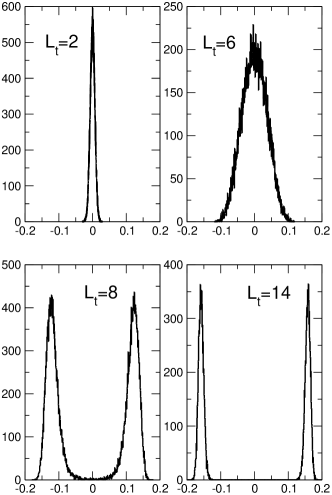
Figure 1: The distribution of the average field for $L_{s}=64$ and four values of $L_{t}$.

Our lattice results show that, well above the phase transition temperature, i.e. for very small $L_{t}$, when the system is in the symmetric phase, the data for the propagator are well reproduced by Eq. (10) down to $p=0$. Therefore, at high temperature the zero-momentum limit is smooth so that $Z_{\varphi}$ and $Z_{\text{prop}}$ agree to very good accuracy, as they do in a $T=0$ symmetric-phase simulation for $\kappa<\kappa_{c}$. Thus the broken-phase discrepancy between $Z_{\varphi}$ and $Z_{\text{prop}}$ is a real physical effect that could be ascribed to the presence of a non-vanishing scalar condensate in the broken phase. In Fig. 2 we have summarized our data for $Z_{\varphi}$. They show a clear increase when $T\to T_{c}$ in contrast with the values of $Z_{\mathrm{prop}}$ (not shown) that remain remarkably close to the zero-temperature value $0.9551$. The trend for $T\to T_{c}$ is in qualitative agreement with our previous zero-temperature study for $\kappa\to\kappa_{c}$.

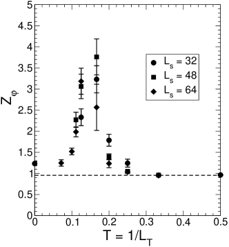
Figure 2: Lattice data for $Z_{\varphi}\equiv m^{2}_{\mathrm{prop}}\chi$ vs. T. Dashed line is the T=0 value $Z_{\mathrm{prop}}=0.9551$.

We stress that the conventional interpretation of ‘triviality’, assuming $Z_{\varphi}=Z_{\mathrm{prop}}\simeq 1$, predicts that approaching the phase transition one should find $m^{2}\to 0$ and $\chi\to\infty$ in such a way that $m^{2}\chi$ remains constant. In this sense, the finite-temperature simulations, showing a dramatic increase of $Z_{\varphi}=2\kappa\chi m^{2}_{\text{prop}}$ when approaching the phase transition, confirm and extend the previous zero-temperature results where the continuum limit was approached by letting $\kappa\to\kappa_{c}$. Both show that $Z_{\varphi}$ is very different from the more conventional quantity $Z_{\text{prop}}\sim 1$ determined perturbatively from the residue of the shifted field propagator. For this reason, the lattice data support once more the alternative picture of Refs. [1, 2] where an infinitesimal curvature of the effective potential $V^{\prime\prime}_{\text{eff}}=M^{2}_{h}/Z_{\varphi}\to 0$ can be reconciled with finite values of $M_{h}$. This non-trivial result may have important consequences for particle physics and cosmology

References

- [1] M. Consoli and P.M. Stevenson, Z. Phys. C63 (1994) 427, hep-ph/9310338.
- [2] M. Consoli and P.M. Stevenson, Int. J. Mod. Phys. A15 (2000) 133, hep-ph/9905427.
- [3] P. Cea et al., Mod. Phys. Lett. A14 (1999) 1673, hep-lat/9902020.
- [4] M. Lüscher and P. Weisz, Nucl. Phys. B295 (1988) 65.