Adaptive Optimization of Wave Functions for
Fermion Lattice Models

Abstract

We present a simulation algorithm for Hamiltonian fermion lattice models. A guiding trial wave function is adaptively optimized during Monte Carlo evolution. We apply the method to the two dimensional Gross-Neveu model and analyze systematc errors in the study of ground state properties. We show that accurate measurements can be achieved by a proper extrapolation in the algorithm free parameters.

Lattice Field Theory is a constructive framework where non-perturbative properties of quantum models can be addressed both analytically and by numerical techniques. The main standing theoretical viewpoints are the traditional Lagrangian approach [1] and the Hamiltonian formulation [2]. In the study of fermionic models, Lagrangian simulations suffer the drawback of requiring Grassmann variables that are difficult to handle numerically and must be integrated out explicitly leading to large non-local determinants. Instead, in the Hamiltonian approach, the treatment of Fermi anticommuting operators is straightforward. In particular, this holds in one spatial dimension where notoriously difficult sign-problems [3] are tame.

Another important reason to resort to Hamiltonian methods is that they rely on powerful well founded Many-Body techniques [4]. In particular, a direct analysis of the ground state structure is often feasible through a guiding trial wave function [5]. This is an approximation to the exact ground state that can provide deep physical insights about the model under consideration. Also, it plays a central role in the simulation algorithms and the quality of the results depends critically on its accuracy [7]. Usually, it contains a set of free parameters that deserve optimization by rather expensive variational calculations [8].

Here, we present a Monte Carlo (MC) algorithm that includes automatic optimization of the trial wave function by means of a non-linear feedback between state sampling and guiding. The MC core is based on a general stochastic representation of matrix evolution problems [9] and has been discussed in the specific case of the Hubbard model [10]. The adaptive optimization strategy has been already applied to Diffusion MC studies of purely bosonic models with continuous state space [5].

In this Report, we focus on fermionic models and present an algorithm suitable for the study of Hamiltonians acting on a finite-dimensional fully discrete state space. In fact, for a local fermion model discretized on a finite lattice, the Hamiltonian is a large sparse matrix $H=\{H_{ss^{\prime}}\}_{s,s^{\prime}\in S}$, with $S$ denoting the discrete state space. The ground state can be obtained by acting on a given initial state with the evolution semigroup $\Omega=\{e^{-tH}\}_{t\geq 0}$ in the $t\to\infty$ limit. For simplicity, we assume a non degenerate ground state, in the general case $\Omega$ projects onto the lowest eigenspace.

To build a MC algorithm, we need a probabilistic representation of $\Omega$. For each pair $s,s^{\prime}\in S$ such that $s\neq s^{\prime}$ and $H_{s^{\prime}s}\neq 0$ we define $\Gamma_{s^{\prime}s}=-H_{s^{\prime}s}$. We assume that all $\Gamma_{s^{\prime}s}>0$ (no sign-problem) and build a $S$-valued Markov stochastic process $s_{t}$ by identifying $\Gamma_{s^{\prime}s}$ as the rate for the transition $s\to s^{\prime}$. Hence, the average occupation $P_{s}(t)=\mbox{\bf E}\left(\delta_{s,s_{t}}\right),$ with $\mbox{\bf E}\left(\cdot\right)$ denoting the average with respect to $s_{t}$, obeys the Master Equation $\dot{P}_{s}(\beta)=\sum_{s^{\prime}\neq s}(\Gamma_{ss^{\prime}}P_{s^{\prime}}-\Gamma_{s^{\prime}s}P_{s}).$

Related to $s_{t}$, we also define the real valued stochastic process $W_{t}=\exp\left(-\int_{0}^{t}\omega_{s_{t}}\ dt\right),$ with $\omega_{s}=\sum_{s^{\prime}\in S}H_{s^{\prime}s}$. It can be shown that the weighted expectation value $\psi_{s}(t)=\mbox{\bf E}\left(\delta_{s,s_{t}}W_{t}\right)$ reconstructs $\Omega$:

$$\frac{d}{dt}\psi_{s}(t)=-\sum_{s^{\prime}\in S}H_{ss^{\prime}}\psi_{s^{\prime}}(t),$$

with $\psi_{s}(0)=\mbox{Prob}(s_{0}=s)$. Matrix elements of $\Omega$ can be identified with certain expectation values. In particular, the ground state energy $E_{0}$ can be obtained by

$$E_{0}=\lim_{t\to+\infty}\frac{\mbox{\bf E}\left(\omega_{s_{t}}\ W_{t}\right)}{\mbox{\bf E}\left(W_{t}\right)},$$ (1)

that gives $E_{0}$ as the asymptotic average of $\omega_{s}$ over realizations of $s_{t}$ with weight $W_{t}$, called walkers in the following. The actual construction of the process is straighforward. A realization of $s_{t}$ is a piece-wise constant map ${\bf R}\to S$ with isolated jumps at times $t=t_{0},t_{1},\dots$, with $t_{0}<t_{1}<t_{2}<\cdots$. An algorithm to compute the triples $\{t_{n},s_{t_{n}},W_{t_{n}}\}$ is the following:

1. We simply denote $s_{t_{n}}\equiv s$ and define the set $T_{s}$ of target states connected to $s$: $T_{s}=\{s^{\prime},\Gamma_{s^{\prime}s}>0\}$. We also define the total width $\Gamma_{s}=\sum_{s^{\prime}\in T_{s}}\Gamma_{s^{\prime}s}$.

2. Extract $\tau\geq 0$ with probability density $p_{s}(\tau)=\Gamma_{s}e^{-\Gamma_{s}\tau}$. In other words, $\tau=-\frac{1}{\Gamma_{s}}\log\xi$ with $\xi$ uniformly distributed in $[0,1]$.

3. Extract a new state $s^{\prime}\in T_{s}$ with probability $p_{s^{\prime}}=\Gamma_{s^{\prime}s}/\Gamma_{s}$.

4. Define $t_{n+1}=t_{n}+\tau$, $s_{t_{n+1}}=s^{\prime}$ and $W_{t_{n+1}}=W_{t_{n}}\cdot e^{-\omega_{s}\tau}$.

The above algorithm is the explicit zero imaginary time limit of power algorithms [14].

For a better performance, it is useful to introduce a trial state $|\Phi(\alpha)\rangle$ depending on some parameters $\alpha$. The original Hamiltonian $H$ is replaced by the isospectral $H_{ss^{\prime}}(\alpha)=\Phi_{s}(\alpha)H_{ss^{\prime}}\Phi_{s^{\prime}}^{-1}(\alpha)$ with $\Phi_{s}(\alpha)=\langle s|\Phi(\alpha)\rangle$. The algorithm is unchanged (hermiticity of $H(\alpha)$ has not been assumed), but everything, in particular $\omega_{s}$, becomes $\alpha$-dependent. In the ideal case when $|\Phi(\alpha)\rangle$ is the exact ground state, then $\omega_{s}\equiv E_{0}$ and the ground state energy is estimated by Eq. (1) with zero fluctuations.

As is well known, a naive implementation of Eq. (1) fails because the variance of the right hand side diverges as $t\to+\infty$. A possible way out is Stochastic Reconfiguration (SR) [11, 12, 13, 14]. An ensemble with a large fixed number $K$ of walkers is introduced and a branching procedure deletes walkers with low weight and makes copies of the ones with larger weight. In the end, we take the numerical limit $K\to\infty$. If $\beta$ is the time between two SR, then we denote the estimate of the ground state energy by $\widehat{E_{0}}(\beta,K,\alpha)$ where we do not write the dependence on physical parameters (lattice size, couplings). Usually, the dependence on $\alpha$ is quite strong and requires optimization to make $|\Phi(\alpha)\rangle$ the closest possible to the exact ground state.

As we remarked, a possible way to optimize $\alpha$ is to minimize the fluctuations of $\omega_{s_{t}}(\alpha)$ [15]. To this aim, following the general ideas of [16], we promote $\alpha$ to a sequence $\{\alpha_{n}\}$ and after each SR, we compute the variance of $\omega(\alpha)$ over the $K$ walkers, with their states kept fixed. Then, we propose to update $\alpha$ according to

$$\alpha_{n+1}=\alpha_{n}-\eta_{n}\nabla_{\alpha_{n}}\mbox{Var}\ \omega(\alpha_{n}).$$ (2)

The sequence $\{\eta_{n}\}$ controls the speed of the adaptive process and vanishes as $n\to\infty$, typically like $n^{-1}$. The novelty of the procedure is that MC sampling and trial wave function optimization are coupled. A change in $\alpha$ induces a change in the walker dynamical distribution which in turn determines the next evolution of $\alpha$. The whole process is non-linear and an explicit numerical investigation is required to assess its stability.

As a specific non-trivial application, we consider the two dimensional Gross-Neveu model [17] described by the Hamiltonian

$$H=\int dx\left[-i\psi^{a\dagger}\sigma_{x}\partial_{x}\psi^{a}-\frac{g^{2}}{2N_{f}}(\psi^{a\dagger}\sigma_{z}\psi^{a})^{2}\right],$$ (3)

where $\psi^{a}$ are $N_{f}$ Dirac fermions and we sum over the repeated flavor index $a=1,\dots,N_{f}$. The model is asymptotically free, admits a $1/N_{f}$ expansion and breaks spontaneously the discrete chiral $Z_{2}$ symmetry $\psi\to\gamma_{5}\psi$.

Following [18], a lattice formulation with staggered Kogut-Susskind fermions [19] is based on

$$H=-\sum_{n=0}^{L-1}\left\{\frac{1}{2}(c_{n}^{a\dagger}c_{n+1}^{a}+\mbox{h.c.})+\frac{g^{2}}{8N_{f}}(c_{n}^{a\dagger}c_{n}^{a}-c_{n+1}^{a\dagger}c_{n+1}^{a})^{2}\right\}$$

where $\{c^{a}_{n},c^{b}_{m}\}=0$, $\{c^{a}_{n},c_{m}^{b\dagger}\}=\delta_{n,m}\delta_{a,b}$ and periodic boundary conditions are assumed. The state space is the set of eigenstates of the occupation number operators $n_{i}^{a}=c_{i}^{a\dagger}c_{i}^{a}$ denoted by $|{\bf n}\rangle$. The fermion number is conserved and we focus on the half-filled sector with $\sum_{i}n_{i}^{a}=L/2$. The $Z_{2}$ symmetry corresponds to translations by two lattice sites. To avoid sign-problems related to boundary crossing we choose in the following $L\ \mbox{mod}\ 4=2$ (the ground state is then non-degenerate).

We adopt the one parameter trial wave function

$$\langle{\bf n}|\Phi(\alpha)\rangle=\exp\left[\alpha\sum_{i=0}^{L-1}(\sum_{a=1}^{N_{f}}(n_{i}^{a}-n_{i+1}^{a}))^{2}\right]\langle{\bf n}|g=0\rangle,$$

where $|g=0\rangle$ is the exact ground state at $g=0$. The algorithm requires an explicit formula for the ratio $\langle{\bf n^{\prime}}|\Phi\rangle/\langle{\bf n}|\Phi\rangle$ where $|{\bf n}\rangle$ and $|{\bf n^{\prime}}\rangle$ are states that differ by one fermion hopping. If $\{x_{i}\}$ and $\{x_{i}^{\prime}\}$ are the $L/2$ fermion positions in the two states and if $x_{i}=x_{i}^{\prime}$ for $i\neq p$, then the following formula can be derived

$$\frac{\langle{\bf n^{\prime}}|\Phi\rangle}{\langle{\bf n}|\Phi\rangle}=e^{\frac{2\pi i}{L}\frac{L/2-1}{2}(x_{p}-x_{p}^{\prime})}\frac{\prod_{k\neq p}\left(\exp\frac{2\pi ix_{p}^{\prime}}{L}-\exp\frac{2\pi ix_{k}}{L}\right)}{\prod_{k\neq p}\left(\exp\frac{2\pi ix_{p}}{L}-\exp\frac{2\pi ix_{k}}{L}\right)}.$$

We compute the ground state energy on a lattice with $L=10$ sites and begin our analysis with the case $N_{f}=2$. We consider several ensemble sizes and evolution times: $K=10$, $50$, $100$ and $500$, $\beta=0.1$, $0.25$, $0.5$ and $1.0$. For each pair $(K,\beta)$ we determine by the adaptive algorithm the best $\alpha$ and estimate the ground state energy. For comparison, we also determine $E_{0}$ by exact Lanczos diagonalization.

Fig. 1 shows the typical initial steps of a run. The parameter $\alpha$ and the energy measurements evolve and fluctuate around $(K,\beta)$ dependent definite average values $\alpha^{*}(K,\beta)$ and $\widehat{E_{0}}(K,\beta,\alpha^{*}(K,\beta))$. For large $K$, the statistical error on $\widehat{E_{0}}$ decreases like $K^{-1/2}$. For $K\to\infty$, the results are expected to be $\beta$ independent. However, for moderate ensemble sizes, like those considered ($K\sim 500$), a residual $\beta$ dependence can be observed, particularly at intermediate coupling, as shown in Fig. 2. This effect is due to the process of walker selection associated to SR. The correct approach is to take the $\beta\to 0$ limit where this effect is expected to be negligible. In Fig. 3, we plot $\widehat{E_{0}}(\beta,500,\alpha^{*}(500,\beta))$ as $\beta$ and $g$ are varied. All the curves converge to zero and, in fact, can be smoothly extrapolated to $\beta\to 0$. The resulting percentual relative error $100|E_{0}-\widehat{E_{0}}|/|E_{0}|$ is very small, well below the permille level (see Tab. (I) for numerical results with 4th order polynomial extrapolation).

For large coupling $g$, the convergence is quite fast. The one-parameter trial wave function is accurate because the ground state is dominated by states with low potential that are easily selected by $|\Phi(\alpha)\rangle$. Relatively small $K$ are then already in the asymptotic regime. For intermediate couplings, $g\sim 2.0$, the convergence is again smooth, but less than linear. For smaller couplings, a good convergence is observed and in fact a precise wave function can obtained with $\alpha^{*}\simeq 0$. The optimal $\alpha^{*}$ at $K=500$, $\beta=0.1$ is shown in Tab. (I).

For $g=2.0$, we explore a tentative 6-parameter trial wave function. Denoting the two fermion flavors by $\uparrow$, $\downarrow$, we use $\langle{\bf n}|\Phi\rangle=e^{\sum_{i}F_{i}}\langle{\bf n}|g=0\rangle$ with $F_{i}=\sum_{k=1}^{3}a_{k}(n_{i}^{\uparrow}n_{i+k}^{\uparrow}+\uparrow\leftrightarrow\downarrow)+\sum_{k=0}^{2}b_{k}(n_{i}^{\uparrow}n_{i+k}^{\downarrow}+\uparrow\leftrightarrow\downarrow).$ The MC automatic determination of the 6 parameters is shown in Fig. 4. The algorithm converges to definite coefficients $\{a,b\}$, but the behavior of $\widehat{E_{0}}$ does not dramatically improve (Fig. 5). Nonetheless, some qualitative remarks can be stressed, as the presence of long range correlations between next to neighbor fermions with the same spin and anti-correlations between fermions with opposite spin.

Since the Gross-Neveu model can be studied non perturbatively in the framework of the $1/N_{f}$ expansion, it is interesting to analyze the algorithm performance with a larger number of flavors. In Fig. 6, we show the results for $N_{f}=6$. The exact value is beyond Lanczos diagonalization and we choose to normalize errors at the $\beta=0.1$, $K=500$ value. A comparison with Fig. 3 reveals that the error as well as its $\beta$ dependence are rather reduced with respect to the previous $N_{f}=2$ case.

In summary, our data shows that a clever extrapolation in the algorithm free parameters $K$ and $\beta$ allows accurate results even with small walker ensembles. This is an important feature for realistic large scale simulations aimed at reaching the continuum limit. Results with large $N_{f}$ suggest that the present algorithm can be a viable numerical technique for other fermionic two-dimensional models where the $1/N_{f}$ expansion applies, like the important case of models with dynamical supersymmetric breaking [20]. In principle, extensions to models with sign-problems are possible and, in fact, progress in the optimization issue has been recently proposed [21] within the considered class of MC algorithms.

TABLE I.: $E_{0}/N_{f}$ for the $L=10$ model with $N_{f}=2$ flavors. $\Delta E=E_{0}^{Lanczos}-E_{0}^{MC}$.

$g$	$\alpha^{*}(500,0.1)$	Exact Lanczos Diagonalization	Polynomial Extrapolation	1000 $|\Delta E/E|$
0.5	0.07638(1)	-3.34904	-3.34908(5)	0.012
1.0	0.31347(5)	-3.71687	-3.71689(5)	0.005
2.0	1.4044(3)	-5.99265	-5.9929(5)	0.03
2.5	2.0575(2)	-8.4526	-8.4524(3)	0.02
3.0	2.6198(2)	-11.6949	-11.6927(3)	0.2

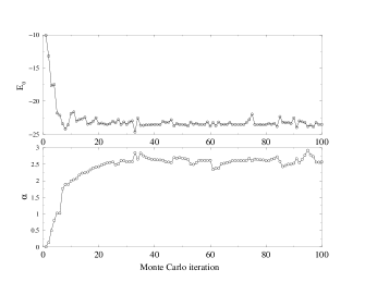
FIG. 1.: $L=10$, $N_{f}=2$, $g=3.0$, $K=10$, $\beta=0.5$. MC evolution of the ground state energy estimate and of the $\alpha$ parameter.

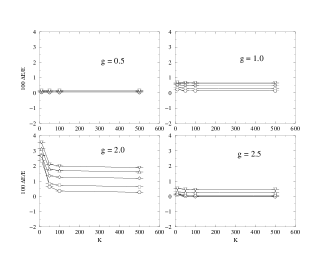
FIG. 2.: $L=10$, $N_{f}=2$. Relative percentual error on the ground state energy. The various lines correspond to $\beta=0.1$ (circles), $\beta=0.25$ (squares), $\beta=0.5$ (diamonds), $\beta=0.75$ (triangles up) and $\beta=1.0$ (triangles down).

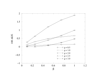
FIG. 3.: $L=10$, $N_{f}=2$, $K=500$. Relative percentual error on the energy obtained from data at large $K$ at several $\beta$.

FIG. 4.: $L=10$, $N_{f}=2$, $g=2.0$. MC evolution of the six parameters $\{a,b\}$. From top to bottom, on the right of the plot, the parameters are $a_{1}$, $a_{3}$, $a_{2}$, $b_{1}$, $b_{2}$, $b_{0}$.

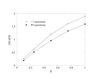
FIG. 5.: $L=10$, $N_{f}=2$, $g=2.0$, $K=500$. Improvement in the energy estimate with the 6-parameter trial wave function.

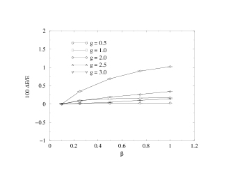
FIG. 6.: $L=10$, $N_{f}=6$, $K=500$. Relative percentual error on the energy estimate obtained from data at large $K$ at several $\beta$.

REFERENCES

- [1] K. Wilson, Phys. Rev. D10, 2445 (1974).
- [2] J. B. Kogut and L. I. Susskind, Phys. Rev. D11, 395 (1975); J. B. Kogut, Rev. Mod. Phys. 51, 659 (1979).
- [3] E. Y. Loh, J. E. Gubernatis, R. T. Scalettar, S. R. White, D. J. Scalapino and R. L. Sugar, Phys. Rev. B41, 9301 (1990).
- [4] W. von der Linden, Phys. Rep. 220, 53 (1992).
- [5] M. Beccaria, Phys. Rev. D61, 114503 (2000); C. Long, D. Robson, S. Chin, Phys. Rev. D37, 3006 (1988);
- [6] M. Beccaria, Phys. Rev. D62, 034510 (2000).
- [7] D. M. Ceperley and M. H. Kalos in Monte Carlo Methods in Statistical Physics, ed. K. Binder, Springer-Verlag, 1992.
- [8] D. Ceperley, G. Chester and M. Kalos, Phys. Rev. B16, 3081 (1977); E. Koch, O. Gunnarsson and R. M. Martin, Phys. Rev. B59, 15632 (1999).
- [9] G. F. De Angelis, G. Jona-Lasinio, M. Sirugue, J. Phys. A16, 2433 (1983).
- [10] M. Beccaria, G.F. De Angelis, C. Presilla, G. Jona-Lasinio, Nucl. Phys. B83-84, (LATTICE 99), 911, (2000); M. Beccaria, G.F. De Angelis, C. Presilla, G. Jona-Lasinio, Europhys. Lett. 48, 243 (1999).
- [11] J. H. Hetherington, Phys. Rev. A30, 2713 (1984).
- [12] S. Sorella, Phys. Rev. Lett. 80, 4558 (1998).
- [13] M. Calandra Buonaura, S. Sorella, Phys. Rev. B57, 11446 (1998).
- [14] S. Sorella,L. Capriotti, Phys. Rev. B61, 2599 (2000).
- [15] C. J. Umrigar, K. G. Wilson and J. W. Wilkins, Phys. Rev. Lett. 60, 1719 (1988); P. R. C. Kent, R. J. Needs and G. Rajagopal, Phys. Rev. B59, 12344 (1999).
- [16] E. Koch, O. Gunnarsson and R. M. Martin, Phys. Rev. B59, 15632 (1999).
- [17] D. J. Gross and A. Neveu, Phys. Rev. D10, 3235 (1974).
- [18] A. Zee, Phys. Rev. D12, 3251 (1975); J. Shigemitsu, S. Elitzur, Phys. Rev. D14, 1988 (1976); J.E. Hirsch, R.L. Sugar, D.J. Scalapino and R. Blankenbecler, Phys. Rev. B26, 5033 (1982); Y. Cohen, S. Elitzur, E. Rabinovici, Phys. Lett. B104, 289 (1981); Y. Cohen, S. Elitzur, E. Rabinovici, Nucl. Phys. B220, 102 (1983).
- [19] L. Susskind, Phys. Rev. D16, 3031 (1977).
- [20] J. L. Goity, Nucl. Phys. B269, 587 (1986); T. Uematsu, Phys. Lett. B123, 209 (1983); T. Uematsu, Phys. Lett. B126, 459 (1983).
- [21] S. Sorella, cond-mat/0009149, Phys. Rev. B, to appear.