An Improved Upper Bound for the Ground State Energy
of Fermion Lattice Models

Abstract

We present an improved upper bound for the ground state energy of lattice fermion models with sign problem. The bound can be computed by numerical simulation of a recently proposed family of deformed Hamiltonians with no sign problem. For one dimensional models, we expect the bound to be particularly effective and practical extrapolation procedures are discussed. In particular, in a model of spinless interacting fermions and in the Hubbard model at various filling and Coulomb repulsion we show how such techniques can estimate ground state energies and correlation function with great accuracy.

In the study of strongly interacting quantum systems, the determination of ground state properties is a basic step in the analysis of many physically relevant problems. To accomplish this task, several powerful numerical methods are available and big efforts have been spent in their development during the last years [1]. However, as is well known, in fermion models, numerical simulations face serious obstructions that dramatically reduce their performance [2]. In this Brief Report, we propose an improved upper bound for the ground state energy and an effective strategy to circumvent this difficulty in a certain class of one dimensional models.

For moderate lattice size, Exact Diagonalization methods are possible [3] with no additional problems in the fermionic case. Typically, these are calculations based on the Lanczos algorithm and the ground state of systems with up to several thousands states can be determined. For larger state space, other methods must be considered. In particular, the most flexible tool is Monte Carlo simulation that evaluates quantum expectation values by a careful stochastic sampling of the configuration space.

Often, when the model under study is fermionic, the measure to be sampled is non-positive. This fact can be related to the intrinsic anticommuting nature of the Fermi creation annihilation operators, but is more general and appears also in bosonic contexts, like quantum spin models with non trivial exchange terms [4]. This situation, usually described as the “sign-problem”, is quite serious and standard algorithms simply fail.

Several proposals are available to overcome or at least reduce the sign problem in specific problems, in particular realistic models in more than one dimension. One of the most powerful techniques is the Constrained Path Monte Carlo Method [5] where the sign problem is eliminated by introducing a physically motivated guiding wave function that approximates the nodal structure of the exact ground state. A numerical analysis is then possible and expectation values can be computed. The approximation is partially controlled and, for instance, the estimates of the ground state energy are known to provide rigorous upper bounds. Other alternatives are the Fixed-Node approximation, the Projection Quantum Monte Carlo, path integral representations or the Auxiliary Field Monte Carlo [6]. Of course, trial wave functions are useful also in cases with no sign problem, but their purpose to accelerate Monte Carlo simulations and the final results are in principle independent on the choice of the guiding function.

Our first goal will be that of providing an improved general upper bound for the energy of fermion lattice models with sign problem; the bound is computable by numerical simulations.

As a second aim, we ask whether one dimensional problems allow for any special simplification and practical treatment of the sign problem in the spirit of [7]. In particular we look for methods that do not rely on any biased approximation. A hint to a positive answer comes from the remark that in one dimension, the sign problem appears to be somewhat artificial. For instance, we can consider a model where the standard fermion hopping term is the unique source of alternating signs in the off diagonal matrix elements of the Hamiltonian. In this case, the sign problem disappears as soon as open boundary conditions are used [8]. Its manifestations are therefore expected to be completely negligible in observable quantities that admit a thermodynamical limit, independent on the boundary conditions. Possible examples are the ground state energy per site and finite correlation lengths. For this reason, we are led to believe that in such cases, the finite size effect of the sign problem should be under control without much effort.

To begin our analysis, let us consider a $d$ dimensional hypercubic lattice with $V=L_{1}L_{2}\cdots L_{d}$ sites and periodic boundary conditions. Let us assign to each site $\bf i$ a pair of spinless fermion creation annihilation operators $c_{\bf i}$ and $c^{\dagger}_{\bf i}$ with canonical algebra

$$\{c_{\bf i},c^{\dagger}_{\bf j}\}=\delta_{{\bf i},{\bf j}},\qquad\{c_{\bf i},c_{\bf j}\}=0,\qquad\{c^{\dagger}_{\bf i},c^{\dagger}_{\bf j}\}=0.$$ (1)

Let us denote a configuration by $\bf n$, the set of occupation numbers at all the lattice sites. We work in the occupation number basis with states $\{|{\bf n}\rangle\}$ such that $c^{\dagger}_{\bf i}c_{\bf i}|{\bf n}\rangle=n_{\bf i}|{\bf n}\rangle$ and assume a given ordering of the sites to fix signs. We want to study Hamiltonians of the form

$$H=H_{kin}+H_{int},$$ (2)

where

$$H_{kin}=-t\sum_{\langle{\bf i},{\bf j}\rangle}(c_{\bf i}^{\dagger}c_{\bf j}+c_{\bf j}^{\dagger}c_{\bf i}),$$ (3)

($\langle{\bf i},{\bf j}\rangle$ denotes a pair of connected sites, for instance nearest neighbours). The interaction term is taken to be diagonal in the $\{|{\bf n}\rangle\}$ basis

$$H_{int}=V({\bf n}),\qquad n_{\bf i}=c_{\bf i}^{\dagger}c_{\bf i},$$ (4)

with $V$ being a real function. The fermion number $N=\sum_{\bf i}n_{\bf i}$ is conserved and the analysis of the spectrum can be carried on in each sector with definite $N$.

In the one dimensional case, $V=L_{1}\equiv L$, we can assume the following canonical site ordering

$$|{\bf n}\rangle=(c_{1}^{\dagger})^{n_{1}}\cdots(c_{L}^{\dagger})^{n_{L}}|{\bf 0}\rangle,$$ (5)

where $|{\bf 0}\rangle$ is the empty state. The paired sites are $\langle i,i+1\rangle$ modulo periodic boundary conditions. The off diagonal matrix elements of $H$ are then negative and Monte Carlo simulations do not have sign problems, except when the fermion number $N$ is even; in this case, there exist matrix elements with the wrong sign, precisely those connecting pairs of states that differ by a hopping through the boundary.

As shown in [9], it is possible to introduce a new Hamiltonian, $H^{\rm eff}$, with no sign problem. Its ground state energy $E_{0}^{\rm eff}$ can be computed by numerical methods and provides a rigorous upper bound for the ground state energy $E_{0}$ of $H$. In [10], this result has been extended by introducing a family of Hamiltonians $\{H(\gamma)\}$ depending on a real free parameter $\gamma$. Let us recall the definition of $H(\gamma)=\{H_{ij}(\gamma)\}$ in terms of $H=\{H_{ij}\}$. We assume $H=DH^{(0)}D^{-1}$ with $H^{(0)}$ hermitean (for instance of the form Eq. (2)) and $D$ diagonal with $D_{ii}\neq 0$. $D$ is a trial wave function useful to accelerate convergence to the ground state. The new Hamiltonian $H(\gamma)$ is given by

$$H_{ij}(\gamma)=\left\{\begin{array}[]{lll}H_{ij}&H_{ij}\leq 0&i\neq j\\ -\gamma H_{ij}&H_{ij}>0&i\neq j\\ H_{ii}+(1+\gamma)\sum_{H_{ik}>0,k\neq i}H_{ik}&&i=j\end{array}\right..$$ (6)

If we call $E_{0}(\gamma)$ the ground state energy of $H(\gamma)$, then it is possible to show that: (i) $E_{0}(-1)=E_{0}$, (ii) $E_{0}(\gamma)\geq E_{0}$ for any $\gamma\geq-1$, (iii) $H(\gamma)$ has no sign problem if $\gamma\geq 0$. In the Monte Carlo approach adopted in [10], it is also emphasized that a strictly positive $\gamma$ must be used and that an extrapolation to $\gamma=0$ is required for best accuracy.

We now show that the function $E_{0}(\gamma)$ is concave in $\gamma$. Namely, for $0\leq\alpha\leq 1$ and any two real $\gamma_{1}$, $\gamma_{2}$, we have

$$E_{0}(\alpha\gamma_{1}+(1-\alpha)\gamma_{2})\geq\alpha E_{0}(\gamma_{1})+(1-\alpha)E_{0}(\gamma_{2}).$$ (7)

A general simple proof can be given by means of the variational characterization of $E_{0}$. The dependence of $H(\gamma)$ on the parameter $\gamma$ is linear and we can write

$$H(\gamma)=DH^{(0)}(\gamma)D^{-1}=D(H_{1}+\gamma H_{2})D^{-1},$$ (8)

with hermitean, $\gamma$ independent $H_{1}$ and $H_{2}$. Then, if $S$ is the set of normalized stated, we have

$$E_{0}(\alpha\gamma_{1}+(1-\alpha)\gamma_{2})=$$ (12)

$$\min_{s\in S}\langle s|\alpha H^{(0)}(\gamma_{1})+(1-\alpha)H^{(0)}(\gamma_{2})|s\rangle\geq$$

$$\geq\alpha\min_{s\in S}\langle s|H^{(0)}(\gamma_{1})|s\rangle+(1-\alpha)\min_{s\in S}\langle s|H^{(0)}(\gamma_{2})|s\rangle=$$

$$\alpha E_{0}(\gamma_{1})+(1-\alpha)E_{0}(\gamma_{2}).$$

Concavity means that the incremental ratio is a decreasing function. Computing the incremental ratio on the intervals $[-1,0]$ and $[\gamma_{1},\gamma_{2}]$ with arbitrary $0\leq\gamma_{1}<\gamma_{2}$ we find

$$E_{0}\leq E_{0}(0)-\frac{E_{0}(\gamma_{2})-E_{0}(\gamma_{1})}{\gamma_{2}-\gamma_{1}}.$$ (13)

If we furthermore assume $E_{0}(\gamma)$ to be differentiable at $\gamma=0$ and take the limit $\gamma_{2},\gamma_{1}\to 0$ we can replace the the upper bound $E_{0}\leq E_{0}(0)$ by the the improved one

$$E_{0}\leq E_{0}(0)-E_{0}^{\prime}(0^{+}),$$ (14)

that expresses the geometrical fact that a concave curve lies below its tangent at any point. We remark that $E_{0}^{\prime}(\gamma)$ can have finite jumps. If they can be excluded a priori, than the above proof follows also by using second order perturbation theory.

The concavity constraint suggests that the function $E_{0}(\gamma)$ could be particularly well behaved. For this reason we also try to obtain an extrapolation of its value at $\gamma=-1$ by assuming it smooth enough. To be fair, this possibility must be considered just a practical recipe. Nonetheless, we shall give numerical arguments to support its robustness.

We begin with a simple model of interacting spinless fermions. The Hamiltonian is

$$H=\sum_{i}\left[-t(c^{\dagger}_{i}c_{i+1}+c^{\dagger}_{i+1}c_{i})\right.+$$ (16)

$$\qquad+\left.V\left(n_{i}-\frac{1}{2}\right)\left(n_{i+1}-\frac{1}{2}\right)\right].$$

For lattice size $L=8$, $12$, $16$ and $20$, at half filling and for several interaction couplings $V$, we determine by Lanczos diagonalization the exact ground state energy $E_{0}$, the bound $E_{0}(0)$, the derivative $\eta=E_{0}^{\prime}(0)$ and the improved bound $E_{0}^{(imp)}=E_{0}(0)-\eta$. Moreover, we also attempt an extrapolation to $\gamma=-1$ starting from the values of $E_{0}(\gamma)$ in the range $\gamma\in(0,1)$. In principle, any such extrapolation can be very dangerous. On the other hand, the extrapolated $E_{0}^{(m)}(-1)$ obtained by a polynomial fit of degree $m$ displays a flat behaviour with small oscillations unless $m$ is too large when the extrapolation process breaks down. The typical degree of the best polynomial is $8$. To accelerate the convergence and to determine the best estimate, we also used Aitkin’s algorithm [11] that improves the converging sequence $\{z_{n}\}$ replacing it with $\{z^{\prime}_{n}\}$ defined by

$$z_{n}^{\prime}=z_{n}-\frac{(\Delta z_{n})^{2}}{\Delta^{2}z_{n}},\quad\Delta z_{n}=z_{n+1}-z_{n},$$ (17)

(where $\Delta^{2}z_{n}=\Delta(\Delta z_{n})$). We call $E_{0}^{(ext)}$ the resulting prediction. In Fig. 1, we show the results for $E_{0}$, $E_{0}(0)$, $E_{0}^{(imp)}$ and $E_{0}^{(ext)}$ in terms of their relative percentual accuracy defined as $100\cdot|\delta E/E_{0}|$ where $\delta E$ is the error in the ground state energy estimate. The improved bound is significantly better than $E_{0}(0)$. Both $E_{0}(0)$ and $E_{0}^{(imp)}$ converge to the exact value as the system size $L\to\infty$ as expected from our initial discussion on the asymptotic irrelevance of the boundary effects. The extrapolated bound $E_{0}^{(ext)}$ is quite precise and around the permille level.

A similar analysis can be done for the measurement of observables. Unfortunately, for these, we cannot derive a simple bound like the one for the energy and in fact random hermitean operators produce easily wild behaviour for $\gamma\in(-1,0)$. On the other hand, for operators associated to physically meaningful quantities independent on the boundary conditions we can expect a mild dependence on $\gamma$. As a typical non local observable, we consider the integrated staggered correlation function defined by

$$S=\frac{1}{L}\sum_{i=1}^{L}\sum_{k=1}^{L/2}(-1)^{k}(\langle n_{i}n_{i+k}\rangle-\langle n\rangle^{2}).$$ (18)

In Fig. 2, we show how the exact values are very accurately reproduced by the extrapolated values. The relative accuracy is always well below the percent level. In Fig. 3, we show the behaviour of the functions $E_{0}(\gamma)$ and $S(\gamma)$ at $V=1$ for the system with $L=16$ together with a 8-th degree polynomial fit to emphasize their smoothness.

For large systems, the upper bound must be computed by numerically extrapolating $E_{0}(0)$ and $E_{0}^{\prime}(0)$. This can be done by a straightforward Monte Carlo simulation at variable $\gamma$. To explore the feasibility of this proposal, we perform such a study for free fermions ($V=0$) on a lattice with $L=40$ sites at half filling. Here, the exact ground state energy is known, $E_{0}/2t=-\cot(\pi/L)\simeq-12.706$ and can be used as a check. We use the Green Function Monte Carlo with Stochastic Reconfiguration [12, 13]. We run simulations with variable number of walkers in order to extrapolate the infinite population size limit. In Fig. 4 we show the estimated value of $E_{0}(\gamma)$ at several positive $\gamma$ values together with a simple parabolic fit. The estimated value of the bound is $E_{0}(0)-E_{0}^{\prime}(0)=-12.61(1)$, about $1\%$ off the exact value.

Similar results are obtained by studying the one dimensional Hubbard model. Denoting by $\uparrow$, $\downarrow$ the two spin degrees of freedom, the Hamiltonian reads

$$H=-t\sum_{i,\sigma=\uparrow,\downarrow}(c^{\dagger}_{i,\sigma}c_{i+1,\sigma}+c^{\dagger}_{i+1,\sigma}c_{i,\sigma})+U\sum_{i}n_{i,\uparrow}n_{i,\downarrow}.$$ (19)

Again, we determine for several lattice size, filling fraction and coupling $U$ the four quantities $E_{0}$, $E_{0}(0)$, $E_{0}^{imp}$ and $E_{0}^{ext}$. The results are shown in Fig. 5 where we show the relative percentual accuracy of $E_{0}^{(ext)}$. The quality of the results is not good as in the spinless model, but the errors are again small, of a few percents. In fact, a scaling analysis shows convergence to the exact values in the large volume limit.

To summarize, the family of Hamiltonian with no sign problem proposed in [10] makes possible the derivation of a size consistent bound for the ground state energy that improves the one at $\gamma=0$. Moreover, much information can be reconstructed for the original Hamiltonian. The accuracy of our analysis on small systems is certainly beyond a practical implementation, but suggests that also for more complicated systems, not allowing a direct analysis, the extrapolated values can provide useful numerical hints. Preliminary results on the two dimensional Hubbard model are encouraging and will be presented elsewhere [14].

Partial support of INFN, Iniziativa Specifica RM42, is acknowledged.

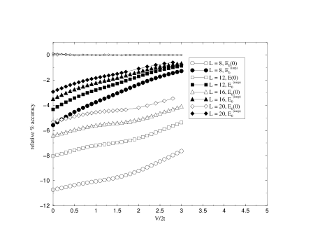
FIG. 1.: Spinless interacting fermions. Relative percentual accuracy of the ground state energy bounds and extrapolated estimate. The circles with very small error are the best extrapolated bound $E_{0}^{(ext)}$ at the various lattice sizes considered $L=8,12,16,20$ (we use the same symbol since the aim is to emphasize the small maximum deviation).

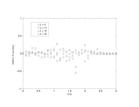
FIG. 2.: Spinless interacting fermions. Relative percentual accuracy of the extrapolated estimate of the integrated staggered correlation function $S$.

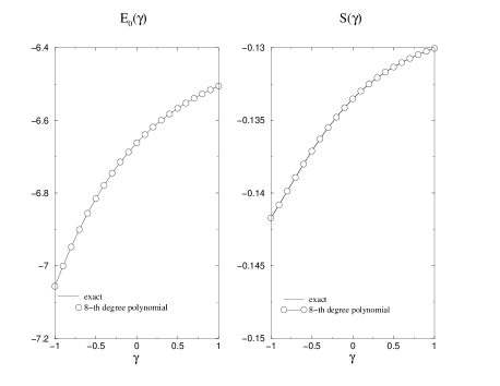
FIG. 3.: Spinless interacting fermions. Smoothness of the function $E_{0}(\gamma)$, $S(\gamma)$ and accuracy of a 8-th degree polynomial fit for the model at $V=1$ with $L=16$ sites.

FIG. 4.: Spinless interacting fermions. GFMC calculation of the effective energy $E_{0}(\gamma)$ in the free case $V=0$, $t=0.5$, on a lattice with $L=40$ sites at half filling. Data are obtained by the GFMC with Stochastic Reconfiguration in the Poisson limit (continuous time). The size of the walker ensemble has been varied from $300$ up to $2000$ and the extrapolation to the infinite population size has been taken. Statistics corresponds to $10^{5}$ reconfigurations separated by an evolution time $\tau=0.5$. The dashed line is a parabolic fit.

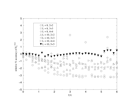
FIG. 5.: Hubbard model. Relative percentual accuracy of the extrapolated estimate of the ground state energy at different sizes, filling and Coulomb coupling.

REFERENCES

- [1] W. von der Linden, Phys. Rep. 220, 53 (1992).
- [2] E. Y. Loh, J. E. Gubernatis, R. T. Scalettar, S. R. White, D. J. Scalapino and R. L. Sugar, Phys. Rev. B41, 9301, (1990).
- [3] E. Dagotto, Rev. Mod. Phys. 66, 763, (1994). For applications in one dimension, mainly with open boundary conditions, a powerful technique is the Density Matrix Renormalization Group, S. R. White, Phys. Rev. Lett. 69,2863, (1992); S. R. White, Phys. Rev. B48, 10345, (1993).
- [4] P. Henelius and A. W. Sandvik, Phys. Rev. B62, 1102, (2000).
- [5] J. Carlson, J. E. Gubernatis, G. Ortiz, S. Zhang, Phys. Rev. B59, 12798, (1999).
- [6] J. B. Anderson, J. Chem. Phys. 65, 4122, (1976); G. Sugiyama, S. .E. Koonin, Ann. Phys. (NY)168, 1, (1986); D. M. Ceperley, Rev. Mod. Phys. 67, 279, (1995); R. Blanckenbecler, D. J. Scalapino, R. L. Sugar, Phys. Rev. D24, 2278, (1981); Phys. Rev. D24, 4295, (1981).
- [7] Y. Alhassid et al., Phys. Rev. Lett. 72, 613, (1994).
- [8] J. Hirsch, D. J. Scalapino, R. L. Sugar and R. Blankenbecler, Phys. Rev. Lett. 47, 1628 (1981); J. Hirsch, D. J. Scalapino, R. L. Sugar and R. Blankenbecler, Phys. Rev. B26, 5033, (1982).
- [9] D. F. B. ten Haaf, H. J. M. van Bemmel, J. M. J. van Leeuwen, W. van Saarlos and D. M. Ceperley, Phys. Rev. B51, 13039, (1995).
- [10] S. Sorella and L. Capriotti, Phys. Rev. B61, 2599, (2000).
- [11] A. C. Aitken, Proc. Roy. Soc. Edinburgh 46, 289 (1926); C. Brezinski, Accélération de la convergence en Analyse Numérique, Springer-Verlag, Berlin, 1977.
- [12] S. Sorella, Phys. Rev. Lett. 80, 4558, (1998); N. Trivedi and D. M. Ceperley, Phys. Rev. B41, 4552, (1990). For a discussion of its continuous evolution time limit see M. Beccaria, C. Presilla, G. F. De Angelis, G. Jona-Lasinio, Europhys. Lett. 48, 243, (1999);
- [13] C. J. Hamer, M. Samaras and R. J. Bursill, Phys. Rev. D62, 074506, (2000); M. Beccaria, Phys. Rev. D62, 034510, (2000).
- [14] M. Beccaria, A. Moro, in preparation.