1 Introduction

The QCD phase transition tightly knits together two of the most intriguing features of QCD: When the temperature drops below the critical value $T_{c}$, chiral symmetry is broken and quarks become confined. State of the art lattice results indicate that both these transitions happen at the same $T_{c}$ (see e.g. [2] for a recent comprehensive review of finite temperature lattice results). Lattice studies which compare the changing behavior of observables on both sides of $T_{c}$ might help to better understand the underlying excitations leading to confinement and chiral symmetry breaking.

While different ideas for excitations responsible for confinement are still heavily debated, the understanding of chiral symmetry breaking seems to be in better shape and during the last 20 years a favorite candidate for the relevant degrees of freedom has emerged. It is now widely believed that models of instanton-like excitations provide a good description of chiral symmetry breaking (for extended reviews see e.g. [3, 4]). These models have a wealth of observable signatures and here we set out to test these predictions in an ab initio lattice calculation and we compare the observables on the two sides of the QCD phase transition.

The basic idea of chiral symmetry breaking from instantons is based on two arguments: Firstly, the Banks-Casher relation [5] (see Eq. (3.1) below) relates the chiral condensate $\langle\overline{\psi}\psi\rangle$ to the density $\rho(\lambda)$ of eigenvalues $\lambda$ of the Dirac operator near to zero. Secondly, the near zero modes which build up the density of eigenvalues $\rho(0)$ at small $\lambda$ are believed to come from interacting instantons and anti-instantons: As long as an instanton is well separated from an anti-instanton, the Dirac operator produces only zero modes which do not contribute to $\rho(0)$ in the Banks-Casher formula. As soon as the instanton and an anti-instanton start to overlap, the Dirac operator can no longer distinguish them as isolated topological objects and instead of two zero modes produces a pair of complex conjugate eigenvalues. For small overlap, these two eigenvalues are still very close to the origin but move up (down) the imaginary axis as the instanton and anti-instanton approach each other.

While earlier studies of instantons on the lattice mainly were based on direct filtering of the gauge fields such as cooling [6], the recent progress for chirally symmetric lattice fermions based on the Ginsparg-Wilson relation [7] now allows to directly use the spectrum and eigenvectors of a chirally symmetric Dirac operator to test the instanton picture (see [8]-[21] for studies of spectrum and eigenvectors of different lattice Dirac operators). When using the eigenvectors of the Dirac operator as a probing tool for instanton-like excitations, the basic assumption is that the localization of the eigenvector traces the localization of the underlying instanton configuration, a property which is known for eigenvectors with eigenvalue 0 of the continuum Dirac operator in an instanton or multi-instanton background. The scenario for chiral symmetry breaking sketched in the last paragraph leads to many characteristic effects that should be visible in the spectrum and eigenvectors of the Dirac operator. In particular the spectral density, the localization of eigenvectors and their local chirality give characteristic signatures which can be tested in an ab initio calculation on the lattice and which might support the instanton picture or rule it out.

In this article we report on our lattice studies of eigenvectors and eigenvalues of the Dirac operator. We use ensembles of SU(3) gauge fields in the quenched approximation. Our runs were done on three different lattice sizes in order to study the volume dependence of observables. The gauge couplings were chosen such that we have ensembles on both sides of the QCD phase transition. This allows to directly compare the changing behavior of observables as one changes from the confined, chirally broken phase to the deconfining, chirally symmetric phase. Such a direct comparison reveals which degrees of freedom show the most drastic changes and thus are relevant excitations for chiral symmetry breaking. Our Dirac operator is an approximate solution of the Ginsparg-Wilson equation based on a systematic expansion [22]-[24] and we will refer to it as the chirally improved Dirac operator. It is considerably cheaper to implement than e.g. the overlap operator [25] while producing very similar results for the relevant eigenvectors and eigenvalues in the physical branch [26]. This property makes the chirally improved Dirac operator ideal for the present study since it allows for very large statistics which would not have been possible for the overlap operator.

We simulate finite temperature QCD by working on a lattice with $L_{t}<L_{s}$, using periodic time boundary conditions for the gauge fields, and antiperiodic for the fermions. The temperature is given by $T=1/L_{t}$.

Let us finally remark on the language convention used in this paper: The short and periodic time-direction $L_{t}$ introduces an additional length scale which is felt by extended excitations of the gauge field. The solution of the SU(3) equations of motion at finite temperature is usually referred to as caloron. Calorons exhibit a string-like localization in time direction. However, the transition between calorons and instantons is continuous, since very small instantons hardly feel the finite time extent. Thus we here use the term topological excitations and speak of instantons or calorons only when we want to stress particular differences.

The article is organized as follows: In the next section we discuss the setting of our computations which encompasses a brief presentation of the chirally improved Dirac operator (Section 2.1), a discussion of the gauge ensembles (Section 2.2) and the techniques used for the diagonalization of the Dirac operator (Section 2.3). In Section 3 we collect our results for the spectrum of the Dirac operator. These results are presented in two parts, Section 3.1 where we discuss the density distribution and Section 3.2 where we analyze the fermionic definition of the topological charge via the index theorem. In Section 4 we present our results for the eigenvectors. In Section 4.1 we give a qualitative discussion based on some examples followed by a discussion of the localization properties of the eigenvectors in Section 4.2. In Section 4.3 we present our results for the local chirality of the eigenvectors. The paper closes with a summary in Section 5. In two appendices we give the details of our Dirac operator (Appendix A) and discuss the fermion zero modes in a classical caloron solution (Appendix B).

2 Preliminaries

2.1 The chirally improved Dirac operator

In the current analysis we use a chirally improved Dirac operator $D$ which is an approximation to a solution of the Ginsparg-Wilson equation [7]. $D$ is a systematic expansion of a Ginsparg-Wilson Dirac operator in terms of paths on the lattice. A detailed description of this approach was presented in [22, 23, 24] and here we only sketch a few basic steps of the construction.

For about three years it has been understood, that chiral symmetry can be implemented through a Dirac operator $D$ which obeys the Ginsparg-Wilson equation [7] (we set the lattice spacing to 1)

$$\gamma_{5}\;D\;\;+\;\;D\;\gamma_{5}\;\;=\;\;D\;\gamma_{5}\;D\;.$$ (2.1)

Currently two types of solutions are known, the so called overlap operator [25] and perfect actions [27, 28]. The overlap operator gives a simple expression for a Dirac operator obeying Eq. (2.1), but the involved square root of a large matrix, makes a numerical evaluation quite costly. In two dimensions the fixed point Dirac operator has been thoroughly tested in the Schwinger model [29]. In four dimensions the perfect Dirac operator has entered the test phase [30], but so far no explicit parametrization has been published.

A third approach to the Ginsparg-Wilson equation is the above mentioned systematic expansion of a solution of Eq. (2.1). The first step in the construction of our chirally improved Dirac operator is to write down the most general Dirac operator on the lattice. This is done by allowing more general lattice discretizations of the derivative. The standard derivative term makes use of nearest neighbors only but certainly one can include also more remote points on the lattice such as next to nearest neighbors or diagonal terms etc. Each such term is characterized by the product of link variables which form the gauge transporter connecting the two points used in the derivative. The corresponding set of links can be viewed as a path on the lattice. The most general derivative on the lattice will then include all possible paths, each of them with some complex coefficient. In order to remove the doublers, in addition to the derivative terms coming with the Dirac matrices $\gamma_{\mu}$ we also have to include terms proportional to the unit matrix in Dirac space. To obtain the most general expression we include all 16 elements $\Gamma_{\alpha}$ of the Clifford algebra, i.e. we also add tensor, pseudovector and pseudoscalar terms. To summarize, our Dirac operator is a sum over all $\Gamma_{\alpha}$, each of them multiplied with all possible paths on the lattice and each path comes with its own coefficient.

The next step is to apply the symmetry transformations: translations, rotations, charge conjugation, parity and $\gamma_{5}$-hermiticity which is defined by

$$D\;\gamma_{5}\;\;=\;\;\gamma_{5}\;D^{\dagger}\;.$$ (2.2)

The property (2.2) can be seen to correspond to the properties of $D$ which are used to prove CPT in the continuum. Once these symmetries are implemented the coefficients of the paths in the Dirac operator are restricted. One finds, that groups of paths which are related by symmetry transformations have to come with the same coefficient, up to possible signs. We denote the most general Dirac operator which obeys the symmetries as:

$$D \!\equiv\mbox{1I}\Big{[}s_{1}\!<>\;+\;s_{2}\!\sum_{l_{1}}<l_{1}>\;+\;s_{3}\!\sum_{l_{2}\neq l_{1}}<l_{1},l_{2}>\;+\;s_{4}\!\sum_{l_{1}}<l_{1},l_{1}>\;...\Big{]}$$

$$+ \sum_{\mu}\gamma_{\mu}\sum_{l_{1}=\pm\mu}s(l_{1})\Big{[}\;v_{1}\!<l_{1}>\;+\;v_{2}\!\sum_{l_{2}\neq\pm\mu}[<l_{1},l_{2}>+<l_{2},l_{1}>]$$

$$\hskip 227.62204pt+\;v_{3}\!<l_{1},l_{1}>\;...\;\Big{]}$$

$$+ \sum_{\mu<\nu}\gamma_{\mu}\gamma_{\nu}\sum_{{l_{1}=\pm\mu\atop l_{2}=\pm\nu}}s(l_{1})\;s(l_{2})\sum_{i,j=1}^{2}\epsilon_{ij}\Big{[}\;t_{1}<l_{i},l_{j}>\;...\;\Big{]}$$

$$+ \!\!\sum_{\mu<\nu<\rho}\gamma_{\mu}\gamma_{\nu}\gamma_{\rho}\!\!\sum_{{l_{1}=\pm\mu,l_{2}=\pm\nu\atop l_{3}=\pm\rho}}\!\!s(l_{1})\;s(l_{2})\;s(l_{3})\sum_{i,j,k=1}^{3}\epsilon_{ijk}\Big{[}\;a_{1}<l_{i},l_{j},l_{k}>\;...\;\Big{]}$$

$$+ \gamma_{5}\!\!\!\!\sum_{{l_{1}=\pm 1,l_{2}=\pm 2\atop l_{3}=\pm 3,l_{4}=\pm 4}}\!\!s(l_{1})\;s(l_{2})\;s(l_{3})\;s(l_{4})\sum_{i,j,k,n=1}^{4}\epsilon_{ijkn}\Big{[}\;p_{1}<l_{i},l_{j},l_{k},l_{n}>\;...\;\Big{]}\;.$$

By $\epsilon$ we denote the totally anti-symmetric tensors with 2,3 and 4 indices. We use the notation $<l_{1},l_{2}\,...\,l_{n}>$ to denote a path of length $n$ and the $l_{i}\in\{-4,-3,-2,-1,1,2,3,4\}$ simply denote the directions of the subsequent links which build up the path. $s(l_{i})$ is an abbreviation for $sign(l_{i})$. With the particular choice for the generators of the Clifford algebra used in Eq. (LABEL:gendirac) (no additional factors of $i$), the coefficients $s_{i},v_{i},t_{i},a_{i},p_{i}$ are real. The expansion parameter for the Dirac operator in Eq. (LABEL:gendirac) is the length of the path since the coefficients in front of the paths decrease in size as the length of the corresponding path increases. A general argument for this behavior can be given and it has been confirmed numerically for the solution presented in [24]. We remark, that an equivalent form of $D$ presented in [28] is the basis for a parametrization of the perfect Dirac operator.

The final step in our construction is to insert the general expression for $D$ into the Ginsparg-Wilson equation. On the left hand side of the Ginsparg-Wilson equation (2.1) some of the terms acquire minus signs, depending on the commutator of the corresponding $\Gamma_{\alpha}$ with $\gamma_{5}$. On the right hand side an actual multiplication of all the terms in D has to be performed. However, using the above notion of a path, the multiplication on the right hand side can be formulated in a algebraic way and then can be evaluated using computer algebra. Once all multiplications are performed one can compare the left and right hand sides of the Ginsparg-Wilson equation. It is important to note that for an arbitrary gauge field different paths, which correspond to different gauge transporters, are linearly independent and can be viewed as elements of a basis. Thus for the two sides of Eq. (2.1) to be equal, the coefficients in front of the same basis elements on the two sides have to agree. When comparing the terms on the two sides, the result is a set of coupled quadratic equations for the expansion coefficients $s_{i},v_{i},t_{i},a_{i},p_{i}$. This set of equations is equivalent to the Ginsparg-Wilson equation. After a suitable truncation of (LABEL:gendirac) to finitely many terms the system can be solved and the result is an approximation to a solution of Eq. (2.1). In addition it is possible to include a dependence on the inverse gauge coupling $\beta_{1}$ through an additional constraint for the coefficients. This step allows to work with less terms in the parametrization. This procedure is similar to the tuning of the mass-like shift which is used to optimize the localization of the overlap operator [31]. An explicit list of the terms used in our parametrization of the Dirac operator and the values of the coefficients $s_{i},v_{i},t_{i},a_{i},p_{i}$ are given in Appendix A.

After a test of the 2-d chirally improved Dirac operator in the Schwinger model with dynamical quarks in [23] the construction was outlined for four dimensions in [22]. A test of a Dirac operator based on this approximation was presented in [24] and it was found that the approximation is particularly good in the physical part of the spectrum. It was found that near the origin the deviation of the eigenvalues from the Ginsparg-Wilson circle is very small. Since in the present study we are interested in the spectrum near the origin, this makes the chirally improved Dirac operator very well suited for the physical questions analyzed here. It is numerically much less demanding than the overlap operator and has a well ordered spectrum near the origin such that spectral densities and the formation of a gap can be studied.

Before continuing with the discussion of the gauge action in the next subsection, let us discuss a general property of the eigenvectors of a Dirac operator $D$ which obeys the $\gamma_{5}$-hermiticity of Eq. (2.2). Let $\psi$ be an eigenvector of $D$, i.e. $D\psi=\lambda\psi$. Then a few lines of algebra show [32]

$$\psi^{\dagger}\;\gamma_{5}\;\psi\;\;=\;\;0\;\;,\;\;\mbox{ unless }\;\lambda\;\mbox{ is real }\;.$$ (2.4)

This equation is the basis for the identification of the zero modes. For the continuum Dirac operator or also for a $D$ which is an exact solution of the Ginsparg-Wilson equation only zero modes have a non-vanishing matrix element with $\gamma_{5}$. Here we are working with an approximate solution of the Ginsparg-Wilson equation and we do not have exact zero modes. However, eigenvectors where the corresponding eigenvalue has a non-vanishing imaginary part are excluded as candidates for zero modes, since their matrix elements with $\gamma_{5}$ vanish exactly. In our approximation the zero modes show up as eigenvectors with a small real eigenvalue and a value of $\psi^{\dagger}\gamma_{5}\psi\sim\pm 0.87$. If one adds more terms in our approximation then the zero modes would be closer to $0$ and the matrix element with $\gamma_{5}$ closer to $\pm 1$.

2.2 The gauge ensembles

The ensembles of gauge configurations for our study were generated with the Lüscher-Weisz action [33, 34]. To be specific, we use the improved gauge action as presented in [34]. Explicitly, the gauge field action reads

$$S[U] = \beta_{1}\sum_{pl}\frac{1}{3}\;\mbox{Re~{}Tr}\;[1-U_{pl}]\;+\;\beta_{2}\sum_{rt}\frac{1}{3}\;\mbox{Re~{}Tr}\;[1-U_{rt}]$$ (2.5)

$$+ \beta_{3}\sum_{pg}\frac{1}{3}\;\mbox{Re~{}Tr}\;[1-U_{pg}]\;,$$

where the first sum is over all plaquettes, the second sum over all $2\times 1$ rectangles and the last sum runs over all parallelograms. $\beta_{1}$ is the principal parameter while $\beta_{2}$ and $\beta_{3}$ can be computed from $\beta_{1}$ using tadpole improved perturbation theory [35], giving [34]

$$\beta_{2}\;=\;-\;\frac{\beta_{1}}{20\;u_{0}^{2}}\;[1+0.4805\,\alpha]\;\;,\;\;\beta_{3}\;=\;-\;\frac{\beta_{1}}{u_{0}^{2}}\;0.03325\,\alpha\;.$$ (2.6)

with

$$u_{0}\;=\;\Big{(}\frac{1}{3}\mbox{Re~{}Tr}\langle U_{pl}\rangle\Big{)}^{1/4}\;\;,\;\;\alpha\;=\;-\;\frac{\ln\Big{(}\frac{1}{3}\mbox{Re~{}Tr}\langle U_{pl}\rangle\Big{)}}{3.06839}\;.$$ (2.7)

The couplings $\beta_{2},\beta_{3}$ are determined self-consistently from $u_{0}$ and $\alpha$ for a given $\beta_{1}$. In Table 1 we list the values of the $\beta_{i}$ used for our ensembles and our results for the expectation value $\langle U_{pl}\rangle/3$ of the plaquette.

$\beta_{1}\;\;$	8.10	8.20	8.30	8.45
$\langle U_{pl}\rangle/3\;\;$	$+0.6294$	$+0.6370$	$+0.6432$	$+0.6521$
$\beta_{2}\;\;$	$-0.5474$	$-0.5499$	$-0.5533$	$-0.5577$
$\beta_{3}\;\;$	$-0.0512$	$-0.0502$	$-0.0495$	$-0.0483$

Table 1: Parameters for our ensembles of gauge field configurations. We list the values of the $\beta_{i}$ and the expectation value $\langle U_{pl}\rangle/3$ of the plaquette.

In [24] it was noted that when comparing the expectation value $\langle U_{pl}\rangle/3$ of the plaquette for the Lüscher-Weisz action with the corresponding expectation value for the Wilson action one finds that the former gives rise to a value of $\langle U_{pl}\rangle/3$ considerably closer to 1 (such a comparison makes sense only after matching a physical scale such as e.g. the string tension). Thus the Lüscher-Weisz action tends to suppress ultraviolet fluctuations and typically one obtains better results for approximate Ginsparg-Wilson fermions [24] as well as for the overlap Dirac operator [36].

For all runs presented here the time extent of the lattice was held fixed at $L_{t}=6$. Our values of $\beta_{1}$ were chosen such that for $\beta_{1}=8.10$ the system is in the confining phase, while the other three values ($\beta_{1}=8.20,8.30,8.45$) are in the deconfined phase. Based on a scaling analysis of the spectral gap [37], we estimate that the phase transition occurs at $\beta_{1}\sim 8.18$.

In order to set the scale we computed the Sommer parameter [38] $r_{0}$ for $\beta_{1}=8.10,8.30$ and $\beta_{1}=8.45$ on $16^{4}$ lattices [39]. We give our results for $r_{0}/a$ together with the lattice spacing $a$ (assuming $r_{0}=0.5$ fm) in Table 2.

Figure 1: The Polyakov loop in the complex plane. Each plot shows 800 measurements for lattice size $6\times 16^{3}$.

In Fig. 1 we show scatter plots of the Polyakov loop [40] $\langle L\rangle$ in the complex plane. For each of our samples we display 800 measurements of $\langle L\rangle$ on a $6\times 16^{3}$ lattice. For $\beta_{1}=8.10$ the measurements of the Polyakov loop are concentrated at the origin indicating that the system is in the confined phase. The other three plots show the emerging of three disjoint clusters of expectation values characteristic for the deconfining phase. The invariance of the pattern under rotations by $2\pi/3$ is due to the Z₃ symmetry of the gauge action. The action for fermions does not display this symmetry and thus fermionic observables behave quite differently in the sector with real Polyakov loop when compared to the two complex sectors [41]. For some of the observables below we will divide our ensembles of gauge field configurations into two sectors according to the phase of the Polyakov loop. We will refer to the configurations where the Polyakov loop $\langle L\rangle$ has a phase $\sim 0$ as the real sector, while configurations with phase $\sim\pm 2\pi/3$ will be referred to as the complex sector.

Finally we comment on the statistics for our runs. For two values of $\beta_{1}$, one in the confining phase ($\beta_{1}=8.10$), the other one in the deconfined phase ($\beta_{1}=8.45$), we performed runs at three different values of the spatial extent $L_{s}$ of our lattice ($L_{s}=12,16,20$) in order to study the finite volume behavior of the system. The temporal extent $L_{t}$ was kept fixed at $L_{t}=6$. To study the $\beta_{1}$-dependence in the deconfined phase we performed two more runs on the $6\times 16^{3}$ lattice at $\beta_{1}=8.20$ and $\beta_{1}=8.30$. In order to compensate for the larger fluctuations on the smaller volumes we analyzed larger samples for these cases. The updates were done with a mix of Metropolis and over-relaxation steps. We also include a random Z₃ rotation in order to update this symmetry of the action. Our configurations are decorelated by roughly two integrated autocorelations times of the Polyakov loop. Table 2 gives an overview over the statistics for our ensembles.

	$\beta_{1}=8.10$	$\beta_{1}=8.20$	$\beta_{1}=8.30$	$\beta_{1}=8.45$
$r_{0}/a$	3.94(16)	-	4.67(13)	5.00(5)
$a$	0.127(5) fm	-	0.107(3) fm	0.100(1) fm
$6\times 12^{3}\;\;$	1200	-	-	1200
$6\times 16^{3}\;\;$	800	800	800	800
$6\times 20^{3}\;\;$	400	-	-	400

Table 2: Sommer parameter $r_{0}$, lattice spacing $a$ and statistics for our gauge field ensembles.

2.3 Technical remarks

For the computation of the eigenvalues and eigenvectors we used the implicitly restarted Arnoldi method [42]. For each of our gauge field configurations we always computed 50 eigenvalues. The search criterion for the eigenvalues was their modulus, i.e. we computed eigenvalues in concentric circles around the origin until 50 were found.

When comparing these eigenvalues for different system sizes, one has to take into account the different density of eigenvalues for different volumes. For larger volumes the Dirac operator has a higher density of eigenvalues than on smaller volumes such that when keeping the number of evaluated eigenvalues fixed at 50, the last eigenvalues found have larger imaginary parts for smaller lattices when compared to the results for larger systems. To give an example, in the chirally broken phase ($\beta_{1}=8.10$) the largest eigenvalues we found among the 50 computed eigenvalues on the smallest lattice ($6\times 12^{3}$) typically had imaginary parts of size $\sim 0.3$ while for the largest lattice ($6\times 20^{3}$) the largest eigenvalues reached only imaginary parts of $\sim 0.14$ (compare the density plots in the next section). Some of our observables are sensitive to these differences due to the technical cut-off of 50 computed eigenvalues and for them we cut off our data at a common physical value for all volumes, i.e. at $|\mbox{Im }\lambda|=0.14$.

3 Results for the spectrum

3.1 Density distribution of the eigenvalues

Along with the transition to the deconfined phase, high temperature QCD also restores chiral symmetry, leading to a vanishing chiral condensate $\langle\overline{\psi}\psi\rangle$. Since the chiral condensate is related to the density $\rho(\lambda)$ of eigenvalues $\lambda$ at $\lambda=0$ via the Banks-Casher formula [5]

$$\langle\overline{\psi}\psi\rangle\;\;=\;\;-\pi\;\rho(0)\;V^{-1},$$ (3.1)

one expects quite a different behavior of the Dirac spectrum on the two sides of the transition. In the deconfined, chirally symmetric phase the density of eigenvalues has to vanish at the origin, up to some zero modes due to isolated topological excitations in the gauge fields. In the confined, chirally broken phase a non-vanishing density of eigenvalues extends all the way to $\lambda=0$.

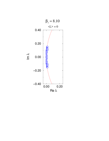
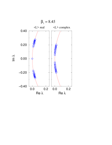
Figure 2: Examples for spectra of the Dirac operator. We show the 50 eigenvalues closest to the origin, represented by circles. All spectra are for $6\times 20^{3}$ lattices. On the left hand side we plot the eigenvalues $\lambda$ in the complex plane for $\beta_{1}=8.10$ (chirally broken phase). The two plots on the right hand side show spectra at $\beta_{1}=8.45$ (chirally symmetric phase) for a gauge configuration with the Polyakov loop in the real sector as well as for a configuration with complex Polyakov loop. The full curve in the plots indicates the Ginsparg-Wilson circle.

In Fig. 2 we show three characteristic spectra, each consisting of the 50 eigenvalues closest to the origin on $6\times 20^{3}$ lattices. For the confining, chirally broken phase ($\beta_{1}=8.10$, left hand side of the plot) we find a non-vanishing density at the origin. When going to the other side of the transition ($\beta_{1}=8.45$, the two plots on the right hand side of Fig. 2) one finds that the spectrum has developed a gap at the origin. There could be some isolated zero modes as e.g. in the central plot but they do not contribute to the density $\rho(\lambda)$ in the Banks-Casher formula (3.1). As already discussed above, the spectrum behaves quite differently for gauge configurations in the real and complex sectors of the Polyakov loop. For the example with the real Polyakov loop (central plot) we find a gap roughly twice as big as for the case with a complex Polyakov loop shown in the plot at the right hand side. There has been some debate whether in the complex sector the gap forms at all [41], but we find that for values of $\beta_{1}$ sufficiently above the critical value the existence of the gap can be clearly established. A detailed analysis of the volume dependence and the scaling of the spectral gap will be presented elsewhere [37].

By averaging over all configurations in each sample (compare Table 2) one can compute the density $\rho(\lambda)$ of eigenvalues. For the continuum Dirac operator the spectrum is restricted to the imaginary axis and the definition of the spectral density is straightforward. For our lattice Dirac operator the spectrum is located on the Ginsparg-Wilson circle, or to be more precise in the vicinity of this circle since here we are dealing only with an approximate Ginsparg-Wilson operator. In order to define the spectral density we bin the eigenvalues with respect to their imaginary part and count the number of eigenvalues in each bin. Eigenvalues with vanishing imaginary part, i.e. the zero modes were left out. After dividing the count in each bin by the total number of eigenvalues we obtain the histograms for $\rho(\lambda)$ used in Fig. 3 below. Since we are only interested in the density $\rho(\lambda)$ in a region of $\lambda$ where the real parts of the eigenvalues on the Ginsparg-Wilson circle are small, binning with respect to the imaginary parts of $\lambda$ gives a good approximation of the continuum definition of the spectral density.

Figure 3: Histogram plots for the spectral density $\rho(\lambda)$ normalized with the inverse volume $V^{-1}$ as a function of Im $\lambda$.

In Fig. 3 we show (see also [10, 11, 12, 13]) the density of eigenvalues $\lambda$ normalized by the inverse volume as a function of Im $\lambda$ (we display only the positive half of the curve, i.e. Im $\lambda>0$). The top plot gives our results for the confined, chirally broken phase. It is obvious that after normalization by the inverse volume, the data for different lattice sizes essentially fall on a universal curve. Only the edge near the origin is more rounded for smaller system size in agreement with universal random matrix theory predictions [43, 44]. For the same reason also the curve for the largest system ($6\times 20^{3}$) still shows a drop near the origin. Up to this finite size effect, the density remains non-zero down to $\lambda=0$, thus building up the chiral condensate according to the Banks-Casher formula (3.1). The picture is quite different in the deconfined, chirally symmetric phase. Again we find that the data for different volumes fall on a universal curve, but now the density drops to zero already at nonvanishing values of Im $\lambda$. For one of our samples ($6\times 16^{3}$) in the real sector (bottom left plot in Fig. 3) we find a very small signal in the vicinity of the origin. We believe that this is a statistically insignificant fluctuation which does not show up for the larger systems. In [12] a similar event on a $4\times 16^{3}$ lattice with Wilson gauge action at $\beta=5.75$ and overlap fermions was observed and interpreted as a possible sign for a non-vanishing fermion condensate in the deconfining phase of quenched QCD.

As already discussed above, the spectral gap is considerably smaller for the sector of gauge configurations with complex Polyakov loop but still is clearly visible (compare also [37]).

3.2 Fermionic definition of the topological charge

In this section we now analyze the zero modes, which for our Dirac operator correspond to eigenvalues with vanishing imaginary part. These modes come from isolated topological excitations of the gauge field. In the continuum the eigenvectors corresponding to the zero modes can be chosen as eigenmodes of $\gamma_{5}$ with eigenvalues $\pm 1$. The numbers $n_{+},n_{-}$ of these left-, respectively right-handed modes are related to the topological charge $Q$ via the Atiyah-Singer index theorem [45]

$$Q\;\;=\;\;n_{+}\;-\;n_{-}\;.$$ (3.2)

A proof of the theorem for the case of a Ginsparg-Wilson lattice Dirac operator can be found in [27]. Here we work only with an approximate solution of the Ginsparg-Wilson equation and we must give a more detailed description of our fermionic definition of the topological charge corresponding to Eq. (3.2).

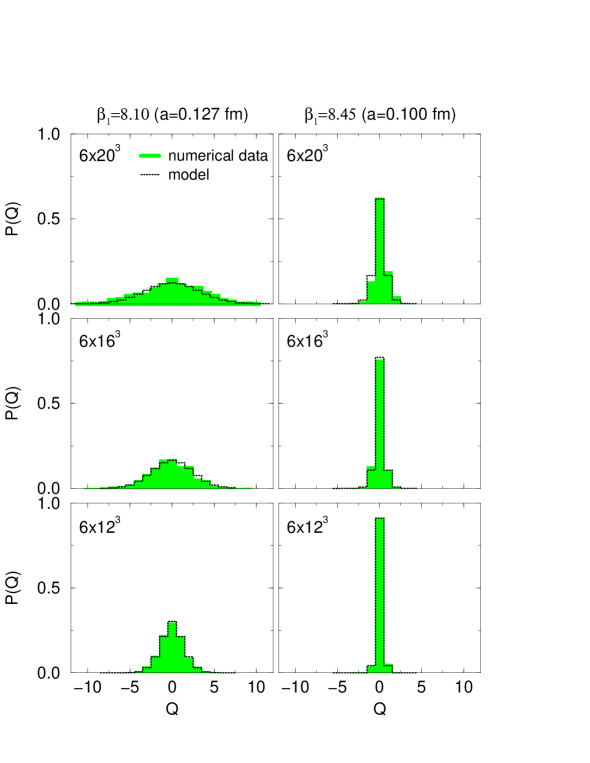
Figure 4: Distribution of the topological charge. The filled histograms show our numerical results and the dotted curve represents the simple instanton anti-instanton model discussed in the text.

There are two main effects of working with only an approximation of a solution of Eq. (2.1): Firstly, the topological modes do not appear at exactly zero, but typically have a small, nonvanishing real part which increases as the corresponding topological excitation of the gauge field becomes more like a defect, i.e. shrinks in size to about a lattice spacing (compare [26]). Secondly, the corresponding eigenvectors $\psi$ are not exact eigenstates of $\gamma_{5}$ but the absolute value of $\psi^{\dagger}\gamma_{5}\psi$ is smaller than 1, typically between $0.8$ and $0.9$ for our $D$. Thus we define $n_{+}$ ($n_{-}$) to be the number of eigenvectors with positive (negative) values of $\psi^{\dagger}\gamma_{5}\psi$ (as noted above $\psi^{\dagger}\gamma_{5}\psi$ vanishes for all eigenvalues with nonvanishing imaginary part (see Eq. (2.4)). In addition we take into account only real eigenvalues smaller than 0.15 in order to discard defects. We should remark, that when moving this cutoff to either 0.10 or 0.20 our results as e.g. shown in Fig. 5 below do not move beyond the error bars. This implies that for our $D$ defects give only a negligible contribution to the fermionic definition of the topological charge.

In Fig. 4 we show our results for the distribution of the topological charge. The filled histograms show our numerical data and the dotted curve is the distribution from a simple model of non-interacting, dilute instantons and anti-instantons.

The basic assumption is that in a cell of size $\delta V$ the probability for finding an instanton or an anti-instanton is given by $\rho_{I}\,\delta V/2$ while the probability for finding an empty cell is $1-\rho_{I}\,\delta V$. Here $\rho_{I}$ is the density of the instantons and anti-instantons which are assumed to be distributed independently. After collecting the combinatorial factors one finds that the probability for having $n_{+}$ instantons and $n_{-}$ anti-instantons is given by a multinomial distribution. This is easily converted to a distribution $P(Q)$ for the topological charge $Q$ as given in Eq. (3.2) by summing over $n_{+}$ and $n_{-}$ with the constraint $\delta(Q-n_{+}+n_{-})$. When going over to the Fourier transform it is straightforward to perform the limit $\delta V\rightarrow 0$ which then gives the integrand in Eq. (3.3) below. Inverting the Fourier transform gives the final result

$$P(Q)\;=\;\frac{1}{2\pi}\int_{0}^{2\pi}dk\;e^{ikQ}\;e^{-\rho_{I}V(1-\cos k)}\;=\;e^{-\rho_{I}V}\;I_{Q}(\rho_{I}V)\;.$$ (3.3)

Here $I_{Q}$ denotes the modified Bessel function of order $Q$ and $V$ is the volume of the system. The expectation value $\langle Q^{2}\rangle$ is then given by

$$\langle Q^{2}\rangle\;=\;2e^{-\rho_{I}V}\;\Big{[}\;I_{1}(\rho_{I}V)\;+\;4\;I_{2}(\rho_{I}V)\;+\;9\;I_{3}(\rho_{I}V)\;...\;\Big{]}\;=\;\rho_{I}\,V\;.$$ (3.4)

Here we used a standard summation formula for the modified Bessel functions. Both results (3.3) and (3.4) depend only on the dimensionless product $\rho_{I}\,V$. Thus as soon as one computes $\langle Q^{2}\rangle$ the distribution $P(Q)$ is entirely fixed. We remark that in this model the topological susceptibility $\chi=\langle Q^{2}\rangle/V$ is simply the density $\rho_{I}$ of instantons and anti-instantons, i.e. $\chi=\rho_{I}$.

A discussion of more sophisticated dilute instanton models, which take interactions into account, can be found in e.g. [46].

When comparing our numerical results to the theoretical prediction (3.3) in Fig. 4 we proceeded as follows: $\langle Q^{2}\rangle$ was first computed for each combination of $\beta_{1}$ and volume (see our results below) and then used to evaluate the theoretical distribution $P(Q)$. Thus the curves shown in Fig. 4 contain no fit. We find that on both sides of the transition and for all system sizes which we analyzed, the numerical data for $P(Q)$ is quite accurately described by the simple instanton anti-instanton model.

Equation (3.4) for $\langle Q^{2}\rangle$ also makes a simple prediction for the volume dependence of $\langle Q^{2}\rangle$. In Fig. 5 we show our results for $\langle Q^{2}\rangle$ as a function of the volume.

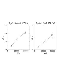
Figure 5: Volume dependence of $\langle Q^{2}\rangle$. The numerical data are represented by diamonds and we connect the symbols to guide the eye. Please note the different scale of the vertical axis in the two plots.

For both phases the volume dependence is roughly linear. For the confined, chirally broken phase ($\beta_{1}=8.10$, left hand side plot) one finds a considerably larger value of the topological susceptibility, i.e. the slope in the plot of $\langle Q^{2}\rangle$ versus $V$ (note the different scales for the two plots). This corresponds to a larger density $\rho_{I}$ in our model. It seems that in the chirally broken phase the assumption of diluteness for the instantons and anti-instantons becomes violated and the topological excitations can no longer be viewed as non-interacting. This may be the reason for the slight deviation from a strictly linear behavior of the $\beta_{1}=8.10$ data. For a more accurate modeling of the $\beta_{1}=8.10$ data the simple model (3.3), (3.4) would have to be augmented by terms describing an interaction of instantons and anti-instantons [4, 46].

Figure 6: $\beta_{1}$-dependence of $\langle Q^{2}\rangle$. The numerical data are represented by filled circles and we connect the symbols to guide the eye. The numbers on the top of the figure give our results for the lattice spacing.

Let us now analyze the $\beta_{1}$-dependence of $\langle Q^{2}\rangle$. It is expected that the chiral susceptibility $\chi=\langle Q^{2}\rangle/V$ drops considerably as one goes from the confining, chirally broken to the deconfined, chirally symmetric phase. In Fig. 6 we show our results for $\langle Q^{2}\rangle$ at $\beta_{1}=8.10,8.20,8.30$ and $8.45$. All data are from $6\times 16^{3}$ lattices such that after a simple rescaling of the vertical axis, Fig. 6 is also a plot for the topological susceptibility. It is obvious that with increasing $\beta_{1}$ the values of $\langle Q^{2}\rangle$, and thus the values of $\chi$, drop considerably. This implies that isolated topological excitations are much rarer in the high temperature phase ($\beta_{1}=8.20,8.30,8.45$) and that their abundance decreases further as one moves away from the critical $\beta_{1}$. This fits nicely into the above discussed picture where the interaction of topological excitations gives rise to the non-vanishing eigenvalue density at the origin $\rho(0)$ in the low temperature phase. Conversely, in the high temperature phase there are simply not enough topological excitations to create a sufficient number of interacting pairs which then would build up a non-vanishing eigenvalue density $\rho(0)$. Of course, the observable $\langle Q^{2}\rangle$ is a measure for the abundance of zero modes, while a non-vanishing $\rho(0)$ is built up from the near zero modes. However, it is quite plausible to assume that as the net number of isolated topological excitations decreases also the number of interacting pairs of topological excitations goes down. In the next section we will confirm this expectation by analyzing an observable which is directly sensitive to the number of interacting pairs.

4 Results for the eigenvectors

4.1 A qualitative discussion of some examples

Before we show our results for the eigenvectors let us first introduce some notation. Eigenvectors will be denoted by $\psi$. They obey the eigenvalue equation

$$D\;\psi\;\;=\;\;\lambda\;\psi\;.$$ (4.1)

The eigenvectors have space, color and Dirac indices which we denote by $x,c$ and $d$ respectively. For each combination of these indices, the corresponding entry $\psi(x,c,d)$ is a complex number. We define a scalar density $p(x)$ and a pseudoscalar density $p_{5}(x)$ by

$$p(x) = \sum_{c,d}\;\psi(x,c,d)^{*}\;\psi(x,c,d)\;$$

$$p_{5}(x) = \sum_{c,d,d^{\prime}}\;\psi(x,c,d)^{*}\;(\gamma_{5})_{d,d^{\prime}}\;\psi(x,c,d^{\prime})\;.$$ (4.2)

Here ^∗ denotes complex conjugation. Note that the summation over the color index makes the densities in Eq. (4.2) gauge invariant. Due to the normalization $\psi^{\dagger}\psi=1$ of the eigenvectors the scalar density sums up to 1, i.e.

$$\sum_{x}\;p(x)\;\;=\;\;1\;.$$ (4.3)

In Fig. 7 we show $x$-$y$ time-slices for the pseudoscalar densities for two characteristic situations (both eigenvectors are for configurations from the $\beta_{1}=8.45$ ensemble on $6\times 16^{3}$ lattices). A similar behavior for the eigenvectors of the staggered Dirac operator was observed in [15]. A study of staggered Dirac operator eigenmodes in finite temperature SU(2), [16], also found localized modes.

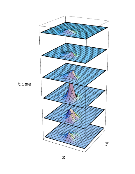
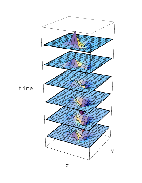
Figure 7: The 6 $x$-$y$ time-slices of the pseudoscalar density $p_{5}(x)$ for a zero mode (top left plot) and a configuration with an interacting caloron anti-caloron pair, a so called topological molecule (bottom right plot). The data are from the $\beta_{1}=8.45$ sample on the $6\times 16^{3}$ lattice.

In the top left plot we display the six (the temporal extent of our lattice is $L_{t}=6$) $x$-$y$ time-slices of $p_{5}(x)$ for an eigenvector with a single real eigenvalue. As already discussed above, these modes correspond to isolated topological excitations which give rise to a zero mode (in our setting an eigenvalue with exactly vanishing imaginary part). Let us discuss some characteristic features of the pseudoscalar density and compare them to the properties known for a classical caloron. For a caloron configuration the corresponding eigenvector (i.e. the zero mode) roughly traces the action density of the gauge configuration, i.e. $p(x)$ is large where $F_{\mu\nu}^{a}(x)F_{\mu\nu}^{a}(x)$ is large. Thus $p(x)$ is localized in space as is the underlying caloron configuration while it is typically more extended in the time direction, where it can interact with itself around the short, compactified time extension of the finite temperature lattice. In addition the eigenvector for a classical caloron is chiral such that $p_{5}(x)=\pm\,p(x)$. The density $p_{5}(x)$ displayed in the top left plot of Fig. 7 shows exactly these features of a zero mode corresponding to a caloron field. The density $p_{5}(x)$ is localized and positive, i.e. in this particular example it corresponds to a caloron which has positive chirality (negative chirality, i.e. $p_{5}(x)<0$ would correspond to an anti-caloron).

In configurations with several calorons we see several non-degenerate real eigenvalues, each having an eigenvector similar to that of the top left plot of Fig. 7. Because the modes are not degenerate, we do not observe strong mixing of the eigenvectors, but instead each of them is essentially tracing only one of the topological excitations. For a Dirac operator which is an exact solution of the Ginsparg-Wilson equation one has exact zero eigenvalues. So in e.g. a two caloron configuration the two zero modes would mix and $p(x)$ and $p_{5}(x)$ would in general show peaks at the positions of both of the calorons.

Let us now turn to an eigenvector which has an eigenvalue with a relatively small but non-zero imaginary part. To be more precise, in the example shown here from the $\beta_{1}=8.45$ ensemble this is a mode at the edge of the spectral gap. According to the caloron picture these modes are due to a pair of a caloron and an anti-caloron which approach each other and start to interact, such that the Dirac operator no longer can distinguish them as two isolated topological excitations and the corresponding two zero modes are split into a complex conjugate pair. We will refer to these configurations of a caloron interacting with an anti-caloron as topological molecule. The dipole structure of such a topological molecule is nicely illustrated in the bottom left plot. The characteristic feature is a positive peak of $p_{5}(x)$ (on the $t=3$ slice) next to a negative peak (on the $t=6$ slice).

Finally we remark, that when inspecting $p_{5}(x)$ for an eigenvector with an eigenvalue in the bulk of the distribution, i.e. an eigenvalue with a large imaginary part one finds that any trace of a localized topological object has been washed out and the pseudoscalar density is dominated by quantum fluctuations.

4.2 Localization properties of the eigenvectors

In the last section we have presented characteristic examples of eigenvectors which display some of the features that are expected from models of topological excitations. In order to go beyond illustrating these properties merely by examples, in this section we now analyze the sample behavior of localization properties of the eigenvectors.

A convenient observable for the localization of an eigenvector is the so-called inverse participation ratio which is widely used in solid state physics. It is defined by

$$I\;\;=\;\;V\;\sum_{x}\;p(x)^{2}\;.$$ (4.4)

Here $V$ denotes the four-volume $L_{t}\,L_{s}^{3}$. From its definition in Eq. (4.2) it follows that $p(x)\geq 0$ for all $x$. Taking into account the normalization Eq. (4.3) one finds that a maximally localized eigenvector which has support on only a single site $x^{\prime}$ must have $p(x)=\delta_{x,x^{\prime}}$. Inserting this into Definition (4.4) for the inverse participation ratio one finds that a maximally localized eigenvector has $I=V$. Conversely, a maximally spread eigenvector has $p(x)=1/V$ for all $x$. In this case, the inverse participation ratio gives a value of $I=1$. Similarly to the scalar inverse participation ratio $I$ of Eq. (4.4) we can also define a measure $I_{5}$ for the localization of the pseudoscalar density $p_{5}(x)$ (see Eq. (4.2)),

$$I_{5}\;\;=\;\;V\;\sum_{x}\;p_{5}(x)^{2}\;.$$ (4.5)

We will refer to $I_{5}$ as the pseudoscalar inverse participation ratio (compare [14] for an alternative observable sensitive to the localization of the pseudoscalar density).

Figure 8: Distribution of the inverse participation ratio.

In Fig. 8 we show the probability distribution $P(I)$ of the inverse participation ratio. We present the results for all lattice sizes of the $\beta_{1}=8.10$ and $\beta_{1}=8.45$ samples, where for the latter case we again distinguish between configurations with a real Polyakov loop and configurations in the complex sector. In order to avoid the problem of different cut-off values for the spectrum when keeping the number of computed eigenvalues fixed at 50 for all lattice sizes (compare the discussion in Section 2.3), the samples for different volumes were cut off at a common value of the imaginary part of the eigenvalues.

A general feature for all plots in Fig. 8 is the increasing probability of finding localized objects (large values of $I$) as the volume gets larger. This is consistent with the property of models of topological excitations which also grow in number as the volume increases. When comparing the distribution in the low temperature phase ($\beta_{1}=8.10$) to the sector of the high temperature phase ($\beta_{1}=8.45$) with real Polyakov loop we do not see a large effect. This means, that the molecules of calorons which form in the chirally symmetric phase still are relatively localized objects. More significant is the change when one compares the plots for the real and complex sector of the Polyakov loop in the chirally symmetric phase ($\beta_{1}=8.45$, the two plots at the bottom of Fig. 8). In the complex sector we find the modes to be much less localized, i.e. the distribution $P(I)$ is much narrower and its peak is shifted to smaller values of $I$. An equivalent dependence of the inverse participation ratio on the Z₃ sector was observed in a study with the staggered Dirac operator in [15]. The dependence of $I$ on the phase of the Polyakov loop can be understood from a property of the classical solutions. Also for a classical caloron one finds that the eigenvector becomes more spread out as one performs a Z₃ transformation of the gauge field which rotates the phase of the Polyakov loop (see Appendix B).

Figure 9: The inverse participation ratio as a function of $|\mbox{Im }\lambda|$.

It is also quite instructive to plot the inverse participation ratio of an eigenvector against its eigenvalue. In Fig. 9 we show such a plot. We binned the imaginary parts Im $\lambda$ of the eigenvalue spectrum and for each bin computed the average size $\langle I\rangle$ of the inverse participation ratio for the corresponding eigenvectors. Eigenvectors which have a real eigenvalue, i.e. the zero modes, were left out. Let us first discuss the plot for the chirally broken phase ($\beta_{1}=8.10$, top plot in Fig. 9). It is obvious that for all lattice sizes, the most localized states (they have the largest values of $I$) sit near Im $\lambda$ = 0. This behavior can again be understood in the context of the picture of a fluid of topological excitations. As already discussed in the last section, the near zero modes are believed to come from pairs of topological excitations which overlap slightly, i.e. large topological molecules. As long as the two excitations are relatively remote, the corresponding eigenvector is still relatively localized, i.e. its $I$ is large. The closer the two partners come the more of their localization is washed out and the corresponding eigenvalue moves away from the origin along the imaginary axis. This behavior is exactly reflected in the plot where the most localized states are near the origin and the localization becomes washed out as one moves along the imaginary axis.

When turning to the chirally symmetric phase ($\beta_{1}=8.45$) the behavior is quite similar. The only difference is the appearance of the gap such that for values of $|\mbox{Im }\lambda|$ below the edge of the gap we find no modes at all. Above the edge, however, we again observe that the most localized states are near the edge and the localization becomes washed out as one moves further away up or down the imaginary axis. For the sector with real Polyakov loop (left hand side plot in the bottom row of Fig. 9) this behavior is quite pronounced, while due to the spreading effect of a Z₃ rotation discussed already above and in Appendix B, the signal is much weaker in the sector with complex Polyakov loop (right hand side plot in the bottom row).

In Section 3 we have seen that $\langle Q^{2}\rangle$ drops considerably as one increases $\beta_{1}$ and goes over to the high temperature phase. $\langle Q^{2}\rangle$ is a measure for the net number of isolated topological excitations. In order to study topological molecules, which do not give rise to zero modes, we analyze the probability for encountering localized modes. We define $N(c)$ to be the number of eigenvectors which are not zero modes (the corresponding eigenvalue is complex and $\psi^{\dagger}\gamma_{5}\psi$ vanishes) and have an inverse participation ratio larger than some cut $c$. Equivalently we define $N_{5}(c)$ to be the number of eigenvectors with a pseudoscalar inverse participation ratio $I_{5}>c$.

In Fig. 10 we show our results for the averages $\langle N(c)\rangle$ and $\langle N_{5}(c)\rangle$ for three different values of $c$. All data were computed on lattices of size $6\times 16^{3}$ and the values of $\beta_{1}$ are $\beta_{1}=8.10,8.20,8.30,8.45$.

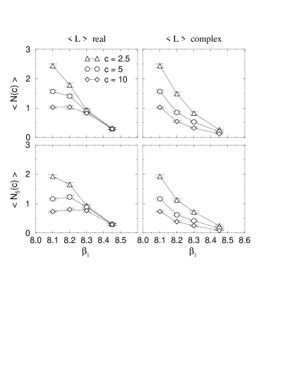
Figure 10: Average of $N(c)$ and $N_{5}(c)$ the numbers of eigenvector with $I>c$ and $I_{5}>c$ respectively, as a function of $\beta_{1}$. Zero modes are omitted in the evaluation of $N(c)$ and $N_{5}(c)$. We display our results from $6\times 16^{3}$ lattices for three values of the cut $c$.

It is obvious, that for all three values of $c$ there is a clear drop of the averages of $N(c)$ and $N_{5}(c)$ for the numbers of eigenvectors with $I>c$ and $I_{5}>c$ respectively, as one increases $\beta_{1}$. As noted above, zero modes were omitted in the evaluation of $N(c)$ and $N_{5}(c)$ such that the observable does not include isolated zero modes and is sensitive only to pairs of topological excitations which, according to the picture of topological molecules build up the eigenvalue density $\rho(0)$ at the origin. The drop of $N(c)$ and $N_{5}(c)$ indicates that the abundance of the topological molecules goes down as $\beta_{1}$ increases. In the high temperature phase their number has become so small that they no longer create a nonvanishing value of $\rho(0)$ and the chiral condensate vanishes.

It is interesting to note that $N(c)$ and $N_{5}(c)$ drop at essentially the same rate. Furthermore this holds individually for both the real and the complex sector of the Polyakov loop even though the shape of the drop is slightly different in the two sectors. This property of a simultaneous drop of the average $N(c)$ and $N_{5}(c)$ further supports the above interpretation that the topological molecules simply become more dilute with increasing $\beta_{1}$ (which causes the drop of $I$) but keep their local chirality (which leads to a decrease of $N_{5}$ at the same rate as the decrease of $N$).

4.3 Local chirality of the eigenmodes

In a recent publication [17] Horváth, Isgur, McCune and Thacker proposed testing the instanton anti-instanton picture of zero temperature QCD by analyzing the local chirality of the eigenmodes of the Dirac operator. If the near zero modes correspond to interacting instantons and anti-instantons, the corresponding peaks in $p(x)$ (compare Eq. (4.2)) should be either left or right handed. An example of this behavior is shown in Fig. 7, where left handed peaks show up as positive values of $p_{5}(x)$ and right handed peaks are negative. However, using the Wilson Dirac operator and a relatively small $\beta$ the authors of [17] did not observe local chirality of their near zero modes. In the meantime their observable has been analyzed by different groups using slightly different settings [18]-[21] and all those later publications do indeed see local chirality supporting the instanton anti-instanton picture.

To clarify this point we also analyzed the local chirality variable of [17]. Before we present our numerical results we briefly repeat the definition of the local chirality variable of [17]. Similar to the densities $p(x)$ and $p_{5}(x)$ of Eq. (4.2) we can now define local densities $p_{+}(x)$ and $p_{-}(x)$ with positive and negative chirality

$$p_{\pm}(x)=\sum_{c,d,d^{\prime}}\;\psi(x,c,d)^{*}\;(P_{\pm})_{d,d^{\prime}}\;\psi(x,c,d^{\prime})\;,$$ (4.6)

where $P_{\pm}$ are the projectors onto positive and negative chirality $P_{\pm}=(1\pm\gamma_{5})/2$. It is now interesting to analyze locally for each lattice point $x$ the ratio $p_{+}(x)/p_{-}(x)$. For a classical instanton in the continuum, the corresponding zero mode $\psi(x)$ has positive chirality and the density $p_{+}(x)$ is positive for all $x$ while $p_{-}(x)$ vanishes everywhere. Thus the ratio of the two always gives $\infty$. For an anti-instanton the roles of $p_{+}$ and $p_{-}$ are exchanged and the ratio is always 0. When now analyzing the eigenvectors for an interacting instanton anti-instanton pair this property should still hold approximately near the peaks. The ratio $p_{+}(x)/p_{-}(x)$ is expected to be large for all $x$ near the instanton peak of the pair and small for all $x$ near the anti-instanton peak. In a final step Horváth et al. map the two extreme values $\infty$ and $0$ of the ratio $p_{+}(x)/p_{-}(x)$ onto the two values $+1,-1$ using the inverse tangent. One ends up with the local chirality variable $X(x)$ defined as

$$X(x)\;=\;\frac{4}{\pi}\;\tan^{-1}\left(\sqrt{\frac{p_{+}(x)}{p_{-}(x)}}\right)\;-\;1\;.$$ (4.7)

When the eigenvectors for the near zero eigenvalues correspond to instanton anti-instanton pairs then the values of $X(x)$ should cluster near $+1$ and $-1$ when one chooses lattice points $x$ near the peaks of the scalar density $p(x)$. One can choose different values for the percentage of points $x$ shown and here we will present results for cuts of 1%, 6.25% and 12.5%. This means that we average over those 1% (6.25%, 12.5%) of all lattice points which support the highest peaks of $p(x)$. The smallest cut-off of 1% will give the best signature since only the highest peaks which are not so much affected by quantum fluctuations do contribute. On the other hand such a small cut-off may not be very conclusive, since typically instanton models have a packing fraction of instantons considerably larger than 1% (see [4, 46]).

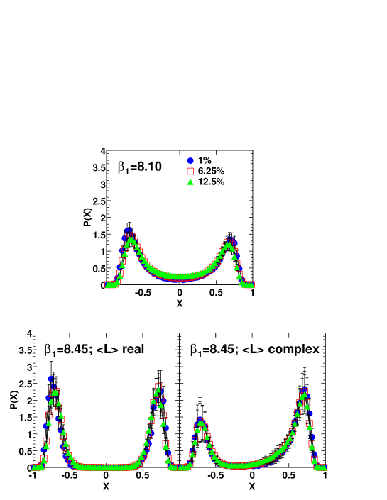
Figure 11: Local chirality for the zero modes. We present data for both sides of the phase transition. For the chirally symmetric phase, we distinguish between the real and the complex sector of the Polyakov loop. We use different values for the cut-off on the percentage of supporting lattice points: 1%, represented by filled circles, 6.25%, open squares and 12.5%, filled triangles. The data were computed on the $6\times 20^{3}$ lattice.

We would like to remark that in [19] a modification of the local chirality variable $X$ was presented, which uses a bi-orthogonal system to construct $p_{\pm}(x)$. This considerably improves the signal for the Wilson Dirac operator. We tested the version proposed in [19] and found only a minor improvement of our results. This is due to the fact that we use an approximation of a Ginsparg-Wilson Dirac operator. A solution of the Ginsparg-Wilson equation is a normal operator which can be diagonalized with a unitary transformation and the bi-orthogonal system then reduces to the right eigenvectors used here.

We start the discussion of the local chirality with the zero modes. In Fig. 11 we show our results for the distribution of $X$ on both sides of the phase transition. The data for the chirally broken phase ($\beta_{1}=8.10$) was computed from 55 gauge configurations. For the chirally symmetric phase ($\beta_{1}=8.45$) we also analyzed 55 gauge configurations but here we distinguish between configurations with real and complex Polyakov loop, such that the sample size for each of the sectors individually is only one third, respectively two thirds of the overall size of 55. In addition, zero modes are much rarer for the $\beta_{1}=8.45$ sample (compare e.g. Fig. 4) and the two effects combined account for the larger error bars in the $\beta_{1}=8.45$ data. We also attribute the slight asymmetry observed in the data for the complex sector of the Polyakov loop to a fluctuation in the relatively small statistics for this plot which seems to contain more left-handed than right-handed modes (compare also Fig. 4). All data we show were computed for the largest volume $6\times 20^{3}$. We remark that our data for $P(X)$ are normalized such that the area under the curve is 1.

All three plots in Fig. 11 show a clear dip of $P(X)$ near $X=0$. Furthermore the shape of $P(X)$ is almost independent of the percentage of lattice points chosen. This shows that zero modes of the Dirac operator are locally chiral up to at least one eighth of the total volume. It is remarkable that the local chirality signal for the zero modes in the chirally broken phase ($\beta_{1}=8.10$) is less pronounced (the two peaks are smaller and wider) than for the zero modes in the chirally symmetric phase. This might be due to the fact that the smaller value of $\beta_{1}$ allows for fluctuations on smaller scales (measured by the number of lattice points) which spoil the signal for local chirality. These UV fluctuations become more suppressed as one increases $\beta_{1}$. Still we can summarize: We find a clear signal for local chirality of the zero modes on both sides of the phase transition.

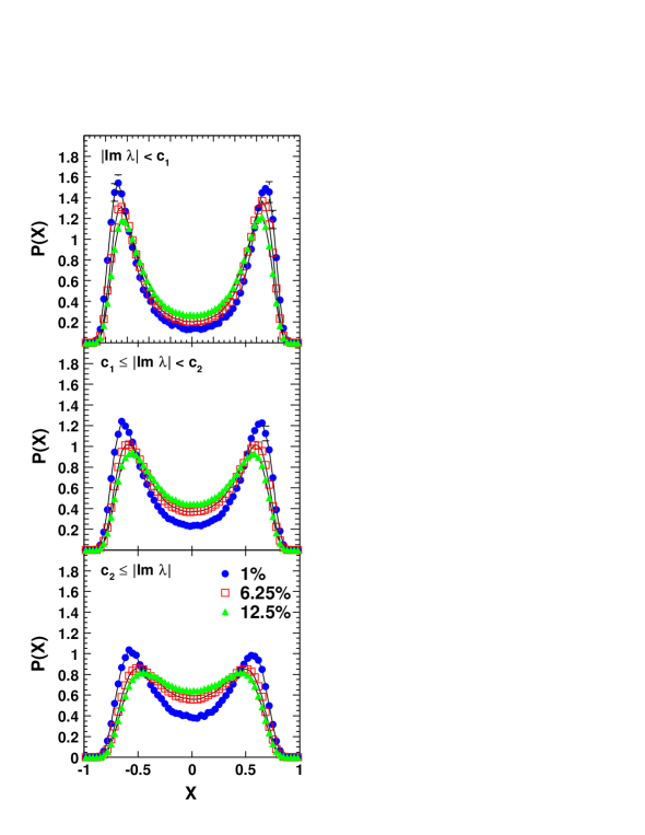
Figure 12: Local chirality for non zero modes in the chirally broken phase. We bin the eigenvectors with respect to the imaginary parts of the corresponding eigenvalues such that the first bin ($|\mbox{Im }\lambda|<c_{1}$, top plot) shows the very near zero modes, while the other two bins ($c_{1}\leq|\mbox{Im }\lambda|<c_{2}$, middle plot and $c_{2}\leq|\mbox{Im }\lambda|$, bottom plot) show the local chirality for eigenvectors with eigenvalues higher up in the spectrum. The choice of the thresholds $c_{i}$ is discussed in the text.

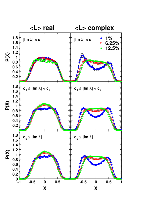
Figure 13: Local chirality for non zero modes in the chirally symmetric phase ($\beta_{1}=8.45,6\times 20^{3}$). We divide our data with respect to the sector of the Polyakov loop. The left column of plots contains the results for real $\langle L\rangle$, the right column shows data for complex $\langle L\rangle$. In addition we bin the data with respect to $|\mbox{Im }\lambda|$ such that the first bin (top plots) shows the local chirality for eigenvectors with eigenvalues close to the edge of the spectral gap, while the other bins (middle and bottom plots) show eigenvectors with eigenvalues more remote from the edge.

Let us now turn to the non zero modes in the chirally broken phase ($\beta_{1}=8.10$). In Fig. 12 we show our results. Again they were computed from 55 gauge configurations on the $6\times 20^{3}$ lattice and we use the same cut-off values as for the zero modes, i.e. 1%, 6.25% and 12.5%. In addition we binned the eigenvectors used for the computation of the local chirality with respect to the imaginary parts of the corresponding eigenvectors. We divided all eigenvectors into three bins such that their eigenvalues obey $|\mbox{Im }\lambda|<c_{1}$ for the first bin, $c_{1}\leq|\mbox{Im }\lambda|<c_{2}$ for the second bin and $c_{2}\leq|\mbox{Im }\lambda|$ for the third bin. The thresholds $c_{i}$ were set such that on the average the first bin contained 4 eigenvectors and the other two bins each 8 eigenvectors (for the computation of the local chirality we always stored a total of 20 eigenvectors which are not zero modes). The values of the $c_{i}$ are given by $c_{1}=0.018$ and $c_{2}=0.057$. The first bin (top plot in Fig. 12) contains the very near zero modes, while in the second and third bin (middle and bottom plots in Fig. 12) we give the results for eigenvectors with larger $|\mbox{Im }\lambda|$.

For the very near zero modes ($|\mbox{Im }\lambda|<c_{1}$, top plot in Fig. 12) we find a very pronounced signal for the local chirality. In fact it is almost indistinguishable from the result for the zero modes shown in the top plot of Fig. 11 (note the different scale on the vertical axis in Fig. 11 and Fig. 12). This shows that the topological molecules responsible for the near zero modes are still very much reminiscent of the localized structure of the two partners, i.e. the caloron and the anti-caloron. Furthermore the dependence for the cut-off on the number of supporting points is very weak, i.e. the 1% and the 12.5% curves are still very similar. This indicates that these modes are relatively spread out, such that, similar to the zero modes, more than one eighth of the volume is occupied by excitations with a definite chirality.

As the eigenvalues move away from the origin, the local chirality of the corresponding eigenvectors becomes less pronounced. This can be seen from the middle and bottom plots in Fig. 12 where we show our results for the second and third bin of $|\mbox{Im }\lambda|$. Firstly we find that the peaks are less pronounced and secondly, that now the curve is much more sensitive to the cut-off for the percentage of supporting lattice points. The interpretation of both these observations is straightforward. According to the instanton picture, eigenvalues higher up in the spectrum are produced by pairs of topological excitations which are overlapping more than the excitations for the near zero modes. Thus the localization for the two partners in a molecule is more washed out and so is the local chirality. This washing out is also reflected in the stronger dependence on the percentage for the supporting lattice points. If the overall height of the peaks in $p(x)$ is going down, then the 1% cut may still see only the highest peaks which are still locally chiral, but the larger values 6.25% and 12.5% start to cut also into the quantum fluctuations which do not have local chirality. To summarize the discussion of Fig. 12, we find good agreement with the picture of topological molecules which produce the nonvanishing eigenvalue density near the origin and lead to eigenvalues higher up (down) in the spectrum as the two partners in the molecule start to overlap more.

Finally we discuss our results for the non zero modes in the chirally symmetric phase ($\beta_{1}=8.45,6\times 20^{3}$). Fig. 13 shows our data which were again divided into the two sectors for the Polyakov loop and the left column of plots shows the sector with $\langle L\rangle$ real and the right column shows the complex sector. As in the chirally broken phase we bin the eigenvectors with respect to the imaginary parts of the corresponding eigenvalues. The first bin ($|\mbox{Im }\lambda|<c_{1}$, top plot in Fig. 13) contains the data for eigenvectors with eigenvalues very close to the edge of the gap, while the other two bins ($c_{1}\leq|\mbox{Im }\lambda|<c_{2}$, middle plot and $c_{2}\leq|\mbox{Im }\lambda|$, bottom plot) show the results for eigenvectors with eigenvalues more remote from the edge. Again we chose the values of the thresholds $c_{i}$ such that the first bin contains an average of 4 eigenvectors while the other two bins each contain 8 eigenvectors. This binning is done for each of the sectors individually. The resulting values for the thresholds at $\beta_{1}=8.45$ are then given by $c_{1}=0.207$ and $c_{2}=0.230$ for the real sector and $c_{1}=0.081$ and $c_{2}=0.112$ for the complex sector.

It is obvious, that for the real sector (left column of plots) the signal for local chirality has vanished entirely. For all three bins and for all three percentages of supporting lattice points we do not see a dip in $P(X)$. This shows that eigenvectors with local chirality do not play a substantial role in the real sector of the chirally symmetric phase at $\beta_{1}=8.45$. Similarly in the data for the complex sector of the Polyakov loop only the 1% cut-off, i.e. only the highest peaks of the scalar density, produces a small dip in $P(X)$, which, however, vanishes as one increases the percentage of supporting points to 6.25% or even 12.5%. Thus only about 1% of the fluctuations in the complex sector of the $\beta_{1}=8.45$ data show local chirality. Based on Fig. 10 and the subsequent discussion we interpret the failure to find non-zero modes with local chirality as further evidence for the diluteness of topological molecules in the chirally symmetric phase.

5 Summary

In this article we have presented a large scale study of eigenvectors and eigenvalues of the lattice Dirac operator. We analyzed the Dirac operator for background gauge fields from quenched finite temperature ensembles on both sides of the QCD phase transition. Using three different lattice sizes we analyzed the volume dependence of our observables. We used a Dirac operator which is an approximate solution of the Ginsparg-Wilson equation and has good chiral properties.

Our observables focused on testing the topological nature of the gauge field excitations as seen by the Dirac operator. In particular we analyzed the density of the eigenvalues, the topological charge defined through the index theorem, scalar and pseudoscalar densities for the eigenvectors, their localization properties and a recently proposed observable for the local chirality of the eigenvectors. Our main results are:

• For the low temperature phase we find a density $\rho(\lambda)$ of eigenvalues which extends all the way to the origin which, according to the Banks Casher relation, gives rise to a non-vanishing chiral condensate in this phase. In the high temperature phase we observe a gap in the spectral density and thus a restoration of chiral symmetry.

• The spectral gap opens up for all phases of the Polyakov loop, i.e. when we divide our ensemble into configurations with real Polyakov loop and configurations where the Polyakov loop has a phase of $\pm 2\pi/3$ we find a gap for both subsets. This shows that the chiral symmetry is restored in both these sectors.

• When analyzing the topological charge $Q$ as defined by the index theorem we find a probability distribution and values of $\langle Q^{2}\rangle$ which can be described well by a simple model of topological excitations. The drop of $\langle Q^{2}\rangle$ as one increases $\beta_{1}$ reflects a thinning out of the topological excitations which prevents the formation of a chiral condensate in the high temperature phase.

• Plots of the pseudoscalar densities for a zero mode and a near zero mode illustrate the characteristic behavior of the different types of excitations.

• A measure for the localization of the eigenvectors is given by the so called inverse participation ratio. For the low temperature phase, we found that the most localized eigenvectors have eigenvalues near the origin and the localization of eigenvectors gets washed out as the imaginary part of the corresponding eigenvalue increases. Similarly one finds for the high temperature phase that the most localized eigenvectors have eigenvalues near the edge of the distribution. These observations support the picture that near zero modes, respectively the near edge modes, are the still relatively localized remnants of interacting calorons and anti-calorons.

• In the high temperature phase we find that the eigenmodes in the Z₃ sector where the Polyakov loop is real are more strongly localized than modes in the complex Z₃ sector. This behavior supports the idea that calorons are relevant, because the classical solution of the Dirac equation in a caloron gauge field shows the same behavior, see Appendix B.

• When plotting the number of eigenvectors with a large localization as a function of $\beta_{1}$ we found a drop when increasing $\beta_{1}$, similar to the drop observed for $\langle Q^{2}\rangle$. This shows that also interacting pairs of calorons and anti-calorons become less abundant at larger $\beta_{1}$ and in the high temperature phase their number is no longer sufficient to build up a non-vanishing chiral condensate.

• Finally we analyzed the local chirality of the eigenvectors at different values of the cut-off for the scalar density. For the chirally broken phase our results for the near zero modes confirm the pattern of local chirality as expected for molecules of topological excitations. In the chirally symmetric phase we still see modes with local chirality near the edge of the gap, but they are much more diluted by bulk modes dominated by quantum fluctuations.

Our results strongly support a picture of interacting topological excitations which are responsible for the breaking of the chiral symmetry at low temperatures, while in the high temperature phase they are no longer sufficiently abundant and the chiral symmetry is restored.

Acknowledgements: We would like to thank Andrei Belitsky, Peter Hasenfratz, Holger Hehl, Ivan Hip, Tamas Kovacs, Christian B. Lang, Ferenc Niedermayer, Edward Shuryak, Wolfgang Söldner and Christian Weiss for interesting discussions. This project was supported by the Austrian Academy of Sciences, the DFG and the BMBF. We thank the Leibniz Rechenzentrum in Munich for computer time on the Hitachi SR8000 and their operating team for training and support.

Appendix A Detailed specification of the chirally improved Dirac operator

In this appendix we describe in more detail the terms in our Dirac operator and give the values for the coefficients which we use for the four ensembles of quenched gauge field configurations.

Clifford generator	Generating path	Name of coefficient
1I	$<>$	$s_{1}$
1I	$<1>$	$s_{2}$
1I	$<1,2>$	$s_{3}$
1I	$<1,2,3>$	$s_{5}$
1I	$<1,1,2>$	$s_{6}$
1I	$<1,2,-1>$	$s_{8}$
1I	$<1,2,3,4>$	$s_{10}$
1I	$<1,2,-1,3>$	$s_{11}$
1I	$<1,2,-1,-2>$	$s_{13}$
$\gamma_{1}$	$<1>$	$v_{1}$
$\gamma_{1}$	$<1,2>$	$v_{2}$
$\gamma_{1}$	$<1,2,3>$	$v_{4}$
$\gamma_{1}$	$<2,1,3>$	$v_{5}$
$\gamma_{1}\gamma_{2}$	$<1,2>$	$t_{1}$
$\gamma_{1}\gamma_{2}$	$<1,2,3>$	$t_{2}$
$\gamma_{1}\gamma_{2}$	$<1,3,2>$	$t_{3}$
$\gamma_{1}\gamma_{2}$	$<1,2,-1>$	$t_{5}$
$\gamma_{1}\gamma_{2}$	$<1,2,-1,-2>$	$t_{15}$
$\gamma_{5}$	$<1,2,3,4>$	$p_{1}$

Table 3: Description of the terms in our $D$.

As has been pointed out in Section 2.1, the most general Dirac operator $D$ can be expanded in the series (LABEL:gendirac). Each term in this series is characterized by three pieces: A generator of the Clifford algebra, a group of paths and a real coefficient. The paths within a group can have different signs which are determined by the symmetries, C, P, $\gamma_{5}$-hermiticity and rotation invariance. The symmetries also determine which paths are grouped together. Thus it is sufficient to characterize a group of paths by a single generating path and all the other paths in the group as well as their relative sign factors can be determined by applying the symmetries.

In addition, for the vector and tensor terms appearing in our $D$ it is sufficient to give the paths only for one vector (tensor) since rotation invariance immediately fixes the structure for the other vector (tensor) terms. In order to describe our $D$ we start with listing the three determining pieces for each term in Table 3.

In Table 4 we list the values of the coefficients $s_{i},v_{i},t_{i}$ and $p_{1}$ for the different values of the inverse gauge coupling $\beta_{1}$ for the ensembles used in this work.

	$\beta_{1}=8.10$	$\beta_{1}=8.20$	$\beta_{1}=8.30$	$\beta_{1}=8.45$
$s_{1}$	$+1.54498$	$+1.54590$	$+1.54688$	$+1.54737$
$s_{2}$	$-0.06169$	$-0.06063$	$-0.05997$	$-0.05892$
$s_{3}$	$-0.01448$	$-0.01449$	$-0.01448$	$-0.01451$
$s_{5}$	$-0.00262$	$-0.00258$	$-0.00255$	$-0.00251$
$s_{6}$	$+0.00220$	$+0.00215$	$+0.00210$	$+0.00206$
$s_{8}$	$-0.00540$	$-0.00534$	$-0.00532$	$-0.00525$
$s_{10}$	$-0.00053$	$-0.00052$	$-0.00051$	$-0.00050$
$s_{11}$	$-0.00118$	$-0.00117$	$-0.00117$	$-0.00116$
$s_{13}$	$+0.00780$	$+0.00778$	$+0.00777$	$+0.00775$
$v_{1}$	$+0.10975$	$+0.11083$	$+0.11063$	$+0.11240$
$v_{2}$	$+0.01770$	$+0.01724$	$+0.01707$	$+0.01654$
$v_{4}$	$+0.00744$	$+0.00767$	$+0.00784$	$+0.00804$
$v_{5}$	$+0.00182$	$+0.00193$	$+0.00198$	$+0.00209$
$t_{1}$	$-0.09874$	$-0.09862$	$-0.09860$	$-0.09843$
$t_{2}$	$-0.00309$	$-0.00303$	$-0.00299$	$-0.00292$
$t_{3}$	$+0.00227$	$+0.00224$	$+0.00221$	$+0.00218$
$t_{5}$	$-0.00663$	$-0.00651$	$-0.00641$	$-0.00627$
$t_{15}$	$-0.00361$	$-0.00358$	$-0.00356$	$-0.00354$
$p_{1}$	$-0.00911$	$-0.00907$	$-0.00905$	$-0.00901$

Table 4: The numerical values of the coefficients $s_{i},v_{i}$, $t_{i}$ and $p_{1}$ for the different ensembles of gauge fields.

Appendix B Quark zero modes

B.1 Solutions of the field equation

In this section we discuss the quark zero modes in the caloron gauge field solutions of Harrington and Shepard [47]. In particular, we want to investigate their dependence on the Z₃ sector.

’t Hooft has shown that one way of generating multi-instanton solutions of the gluon equations of motion is to consider gauge fields of the form

$$A^{\mu}_{cc^{\prime}}(x)=i{\bar{\sigma}}^{\mu\nu}_{cc^{\prime}}\;\partial_{\nu}\ln\rho(x)\;,$$ (B.1)

where $c$ and $c^{\prime}$ are color indices and the ${\bar{\sigma}}$ are a set of $2\times 2$ color matrices. A suitable basis for the ${\bar{\sigma}}$ is given in [48]. After a little algebra one finds that this $A$ field satisfies the equations of motion if

$$\partial^{2}\rho(x)=0$$ (B.2)

$${\rm or}\quad \partial^{2}\rho(x)\propto\rho^{3}(x)\,.$$ (B.3)

We know from the Atiyah-Singer index theorem that gauge field configurations with topological charge must have fermion zero modes. Following [48] these modes can be written in a form analogous to (B.1),

$$\psi_{cd}(x)=\rho^{1/2}(x)\;\alpha^{\mu}_{cd}\,\partial_{\mu}\left(\frac{\chi(x)}{\rho(x)}\right)\;,$$ (B.4)

where $c$ is a color index, and $d$ a Dirac index. The relation of the $\alpha$ matrices to the ${\bar{\sigma}}$ matrices, and a choice of $\alpha$ is given in [48]. The ansatz (B.4) gives a zero mode of the Dirac operator if

$$\rho(x)\,\partial^{2}\chi(x)-\chi(x)\,\partial^{2}\rho(x)=0\,.$$ (B.5)

We now need a solution of Eq. (B.2) that also satisfies the periodic boundary condition in the time direction,

$$\rho(\vec{r},t+1/T)=\rho(\vec{r},t)\;,$$ (B.6)

where $T$ is the temperature (we have set Boltzmann’s constant to 1). A simple solution of this type, [47], is

$$\rho(\vec{r},t)=1+\sum_{k=-\infty}^{\infty}\frac{R^{2}}{r^{2}+(t-k/T)^{2}}=1+\,\frac{\pi TR^{2}\;\sinh(2\pi Tr)}{r\left[\cosh(2\pi Tr)-\cos(2\pi Tt)\right]}$$ (B.7)

where $r^{2}\equiv r_{1}^{2}+r_{2}^{2}+r_{3}^{2}$. This solution corresponds to a caloron of radius $R$ sitting at the origin. We can use translation invariance to give solutions at other locations, and add together solutions of the above form to get multi-caloron solutions.

We now look for a fermion zero mode in the solution (B.7), which should obey anti-periodic boundary conditions

$$\psi(\vec{r},t+1/T)=-\psi(\vec{r},t)\;.$$ (B.8)

$\psi$ depends linearly on $\chi$, so $\chi$ must obey the same boundary conditions as $\psi$. The function

$$\chi(\vec{r},t) = \frac{1}{2\pi}\sum_{k=-\infty}^{\infty}(-1)^{k}\;\frac{R}{r^{2}+(t-k/T)^{2}}$$ (B.9)

$$= \frac{TR\;\cos(\pi Tt)\;\sinh(\pi Tr)}{r\left[\cosh(2\pi Tr)-\cos(2\pi Tt)\right]}\;,$$

satisfies eq. (B.5), and has the correct behavior under $t\to t+1/T$. This has the same form as the general multi-instanton solution given in [49].

The solution (B.9) corresponds to the real sector of the Z₃ symmetry. We are also interested in knowing what the zero-mode looks like in the complex sectors. There are two possible approaches to this problem.

The direct approach is to use the fact that eq. (B.1) gives an SU(2) $A$-field. When we embed this solution in SU(3) the $A$-field has components proportional to the three generators $t^{1},t^{2},$ and $t^{3}$ of SU(3). The generator $t^{8}$ commutes with these three matrices, so we still have a solution of the equation of motion if we add an arbitrary constant $A$ field in the 8-direction of SU(3). This can be used to produce a caloron solution with an arbitrary Polyakov loop value. See [50] for methods of constructing SU(2) solutions with non-trivial Polyakov loop.

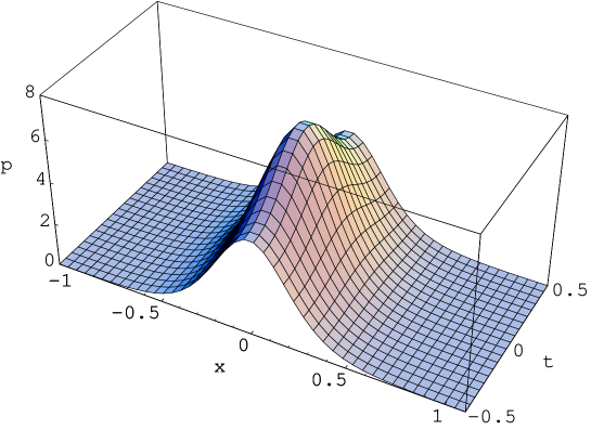
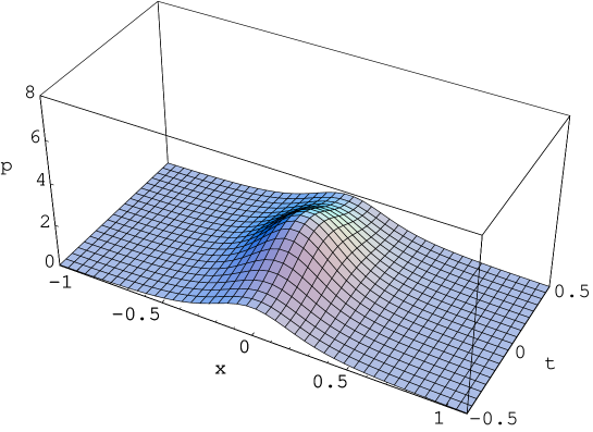
Figure 14: The scalar density $p(x)$ for a quark zero mode in the real Z₃ sector (upper plot) and the complex Z₃ sector (lower plot). In both cases the caloron radius is $1/T$.

A simpler method is to note that a Polyakov loop can be gauge transformed to look just like a fermion boundary condition of the form

$$\psi(\vec{r},t+1/T)=-e^{i\theta}\psi(\vec{r},t)\,.$$ (B.10)

For the complex Z₃ sectors of high-temperature QCD we are interested in $\theta=\pm 2\pi/3$. A solution of eq. (B.5) that obeys Eq. (B.10) is given by

$$\chi(\vec{r},t)=\frac{1}{2\pi}\sum_{k=-\infty}^{\infty}(-1)^{k}e^{ik\theta}\;\frac{R}{r^{2}+(t-k/T)^{2}}$$

$$= \frac{e^{i\theta Tt}TR\left[\cosh(\theta Tr)\cos(\pi Tt)\sinh(\pi Tr)-i\sinh(\theta Tr)\sin(\pi Tt)\cosh(\pi Tr)\right]}{r\left[\cosh(2\pi Tr)-\cos(2\pi Tt)\right]},$$

valid for $-\pi\leq\theta\leq\pi$. At large $r$ the probability density found from eq. (B.1) drops off like $r^{-2}\exp[-2(\pi-|\theta|)Tr]$. This is much faster in the real sector ($\theta=0$) than in the complex sectors ($\theta=\pm 2\pi/3$).

B.2 Phenomenological implications

To illustrate the difference between the Z₃ sectors, we plot the density of the fermion zero mode in a caloron of radius $R=1/T$, see Fig. 14. We show a two-dimensional $x$-$t$ slice through the center of the mode. Both modes have been normalized so that the 4-dimensional integral of $p$ is $1$. One sees clearly that the mode in the real sector is more strongly localized.

Figure 15: The inverse participation ratio $I$ of the quark zero-mode calculated for a caloron in the real Z₃ (solid line) and in the complex sector (dashed line). For comparison the result for an instanton is shown as the dotted line. $R$ is the radius of the caloron and $T$ the temperature.

A systematic way to compare the localization of the modes (B.9) and (B.1) is to define an inverse participation ratio analogous to that of Section 4. The scalar density $p(x)$ is defined in exactly the same way in the continuum as on the lattice, Eq. (4.2). In the definition of $I$ we simply replace the sum in Eq. (4.4) by an integral:

$$I/V\equiv\int d^{4}x\;p(x)^{2}\;$$ (B.12)

where the eigenmode has been normalized so that $\int d^{4}x\;p(x)=1$.

In Fig. 15 we compare the localization of the quark zero modes as the caloron radius $R$ is varied. When $RT\ll 1$ thermal effects are small, so a caloron looks very like an instanton, and the $I$ of the zero mode has only a slight dependence on the Z₃ sector. This contrasts with the situation when the caloron radius is comparable with the inverse temperature, $RT\sim 1$. Here the Z₃ sector has a dramatic effect, with localization being much stronger in the real sector than in the complex. This is reminiscent of the effects we see in the high temperature phase (see Section 4).

References

- [1]
- [2] F. Karsch, hep-lat/0103314.
- [3] D. Gross, R. Pisarski and L. Yaffe, Rev. Mod. Phys 53 (1981) 43.
- [4] T. Schäfer and E.V. Shuryak, Rev. Mod. Phys. 70 (1998) 323; D. Diakonov, Talk given at International School of Physics, ’Enrico Fermi’, Course 80: Selected Topics in Nonperturbative QCD, Varenna, Italy, 1995, hep-ph/9602375.
- [5] T. Banks and A. Casher, Nucl. Phys. B169 (1980) 103.
- [6] M. C. Chu, J. M. Grandy, S. Huang and J. W. Negele, Phys. Rev. D 49 (1994) 6039; J.W. Negele, Nucl. Phys. Proc. Suppl. 73 (1999) 92; D. A. Smith and M. J. Teper, Phys. Rev. D 58 (1998) 014505; U. Sharan and M. Teper, Phys. Rev. D 60 (1999) 054501; P. de Forcrand, M. Garcia Perez and I. Stamatescu, Nucl. Phys. B 499 (1997) 409; T. DeGrand, A. Hasenfratz and T. G. Kovacs, Nucl. Phys. B 505 (1997) 417; Nucl. Phys. B 520 (1998) 301; Phys. Lett. B 420 (1998) 97; M. Garcia Perez, A. Gonzalez-Arroyo, A. Montero and P. van Baal, JHEP 9906 (1999) 001; I. O. Stamatescu and C. Weiss, Nucl. Phys. Proc. Suppl. 94 (2001) 532.
- [7] P.H. Ginsparg and K.G. Wilson, Phys. Rev. D 25 (1982) 2649.
- [8] T. L. Ivanenko and J. W. Negele, Nucl. Phys. Proc. Suppl. 63 (1998) 504; J. W. Negele, Nucl. Phys. A 670 (2000) 14.
- [9] C. Gattringer and I. Hip, Nucl. Phys. B 536 (1998) 363; Nucl. Phys. B 541 (1999) 305.
- [10] T. G. Kovacs, Phys. Rev. D 62 (2000) 034502.
- [11] F. Farchioni, P. de Forcrand, I. Hip, C.B. Lang and K. Splittorff, Phys. Rev. D 62 (2000) 014503.
- [12] R.G. Edwards, U.M. Heller, J. Kiskis and R. Narayanan, Phys. Rev. D 61 (2000) 074504.
- [13] P. H. Damgaard, U. M. Heller, R. Niclasen and K. Rummukainen, Phys. Lett. B 495 (2000) 263.
- [14] T. DeGrand and A. Hasenfratz, Phys. Rev. D 64 (2001) 034512.
- [15] M. Göckeler, P.E.L. Rakow, A. Schäfer, W. Söldner and T. Wettig, Phys. Rev. Lett. 87 (2001) 042001.
- [16] S. Hands, Nucl. Phys. B329 (1990) 205.
- [17] I. Horváth, N. Isgur, J. McCune and H. B. Thacker, hep-lat/0102003.
- [18] T. De Grand and A. Hasenfratz, hep-lat/0103002.
- [19] I. Hip, Th. Lippert, H. Neff, K. Schilling and W. Schroers, hep-lat/0105001.
- [20] R.G. Edwards and U.M. Heller, hep-lat/0105004.
- [21] T. Blum, N. Christ, C. Cristian, C. Dawson, X.Liao, G. Liu, R. Mawhinney, L. Wu and Y. Zhestkov, hep-lat/0105005.
- [22] C. Gattringer, Phys. Rev. D 63 (2001) 114501.
- [23] C. Gattringer and I. Hip, Phys. Lett. B 480 (2000) 112.
- [24] C. Gattringer, I. Hip and C.B. Lang, Nucl. Phys. B597 (2001) 451.
- [25] R. Narayanan and H. Neuberger, Phys. Lett. B 302 (1993) 62, Nucl. Phys. B 443 (1995) 305.
- [26] C. Gattringer, M. Göckeler, C.B. Lang, P.E.L. Rakow and A. Schäfer, hep-lat/0108001.
- [27] P. Hasenfratz, Nucl. Phys. B (Proc. Suppl.) 63 (1998) 53; P. Hasenfratz, Nucl. Phys. B 525 (1998) 401; P. Hasenfratz, V. Laliena and F. Niedermayer, Phys. Lett. B 427 (1998) 353.
- [28] P. Hasenfratz, S. Hauswirth, K. Holland, Th. Jörg, F. Niedermayer and U. Wenger, Int. J. Mod. Phys. C 12 (2001) 691.
- [29] C.B. Lang and T.K. Pany, Nucl. Phys. B 513 (1998) 645; F. Farchioni, C.B. Lang and M. Wohlgenannt, Phys. Lett. B 433 (1998) 377; F. Farchioni, I. Hip, C.B. Lang and M. Wohlgenannt, Nucl. Phys. B 549 (1999) 364.
- [30] P. Hasenfratz, S. Hauswirth, K. Holland, T. Jörg, F. Niedermayer and U. Wenger, Nucl. Phys. Proc. Suppl. 94 (2001) 627.
- [31] P. Hernandez, K. Jansen and M. Lüscher, Nucl. Phys. B 552 (1999) 363.
- [32] S. Itoh, Y. Iwasaki and T. Yoshié, Phys. Rev. D36 (1987) 527, Phys. Lett. B 184 (1987) 375.
- [33] M. Lüscher and P. Weisz, Commun. Math. Phys. 97 (1985) 59; Erratum: 98 (1985) 433; G. Curci, P. Menotti and G. Paffuti, Phys. Lett. B 130 (1983) 205, Erratum: B 135 (1984) 516.
- [34] M. Alford, W. Dimm, G.P. Lepage, G. Hockney and P.B. Mackenzie, Phys. Lett. B 361 (1995) 87.
- [35] G.P. Lepage and P.B. Mackenzie, Phys. Rev. D 48 (1993) 2250.
- [36] K.F. Liu, S.J. Dong, F.X. Lee and J.B. Zhang, Nucl. Phys. Proc. Suppl. 94 (2001) 752.
- [37] C. Gattringer, M. Göckeler, P.E.L. Rakow and A. Schäfer, in preparation.
- [38] R. Sommer, Nucl. Phys. B 411 (1994) 839; M. Guagnelli, R. Sommer and H. Wittig, Nucl. Phys. B 535 (1998) 389.
- [39] C. Gattringer, M. Göckeler, P.E.L. Rakow, S. Schaefer and A. Schäfer, hep-lat/0107016 (Nucl. Phys. B, in print).
- [40] A. M. Polyakov, Phys. Lett. 72 B (1978) 477; B. Svetitsky and L.G. Yaffe, Nucl. Phys. B 210 [FS6] (1982) 423.
- [41] S. Chandrasekharan and N.H. Christ, Nucl. Phys. B (Proc. Suppl.) 47 (1996) 527; P.N. Meisinger and M.C. Ogilvie, Phys. Lett. B 379 (1996) 163; S. Chandrasekharan and S. Huang, Phys. Rev. D 53 (1996) 5100; M.A. Stephanov, Phys. Lett. B 375 (1996) 249.
- [42] D.C. Sorensen, SIAM J. Matrix Anal. Appl. 13 (1992) 357; R. B. Lehoucq, D.C. Sorensen and C. Yang, ARPACK User’s Guide, SIAM, New York, 1998.
- [43] T. Guhr, A. Müller-Groeling and H. A. Weidenmüller, Phys. Rept. 299 (1998) 189.
- [44] M.E. Berbenni-Bitsch, S. Meyer, A. Schäfer, J.J.M. Verbaarschot and T. Wettig, Phys. Rev. Lett. 80 (1998) 1146; J.C. Osborn and J.J.M. Verbaarschot, Phys. Rev. Lett. 81 (1998) 268; R. G. Edwards, U. M. Heller, J. Kiskis and R. Narayanan, Phys. Rev. Lett. 82 (1999) 4188; P.H. Damgaard, U.M. Heller and A. Krasnitz, Phys. Lett. B 445 (1999) 366; M. Göckeler, H. Hehl, P.E.L. Rakow, A. Schäfer and T. Wettig, Phys. Rev. D 59 (1999) 094503; M.E. Berbenni-Bitsch et al., Phys. Lett. B 438 (1998) 14.
- [45] M. Atiyah and I.M. Singer, Ann. Math. 93 (1971) 139.
- [46] D.I. Diakonov and V.Y. Petrov, Nucl. Phys. B 245 (1984) 259; D. Diakonov, M. V. Polyakov and C. Weiss, Nucl. Phys. B 461 (1996) 539.
- [47] B.J. Harrington and H.K. Shepard, Phys. Rev. D 17 (1978) 2122.
- [48] R. Jackiw and C. Rebbi, Phys. Rev. D 16 (1977) 1052.
- [49] B. Grossman, Phys. Lett. A 61 (1977) 86; H. Osborn, Nucl. Phys. 140 (1978) 45.
- [50] T.C. Kraan and P. van Baal, Nucl. Phys. B 533 (1998) 627; T.C. Kraan and P. van Baal, Phys. Lett. B 428 (1998) 268; K.Y. Lee and C. Lu, Phys. Rev. D 58 (1998) 025011.