UTCCP-P-104 Light Hadron Spectroscopy with Two Flavors of Dynamical Quarks on the Lattice

Abstract

We present results of a numerical calculation of lattice QCD with two degenerate flavors of dynamical quarks, identified with up and down quarks, and with a strange quark treated in the quenched approximation. The lattice action and simulation parameters are chosen with a view to carrying out an extrapolation to the continuum limit as well as chiral extrapolations in dynamical up and down quark masses. Gauge configurations are generated with a renormalization-group improved gauge action and a mean field improved clover quark action at three values of $\beta=6/g^{2}$, corresponding to lattice spacings of $a\approx 0.22$, 0.16 and 0.11 fm, and four sea quark masses corresponding to $m_{\rm PS}/m_{\rm V}\approx 0.8$, 0.75, 0.7 and 0.6. The sizes of lattice are chosen to be $12^{3}\times 24$, $16^{3}\times 32$ and $24^{3}\times 48$ so that the physical spatial size is kept constant at $La\approx 2.5$ fm. Hadron masses, light quark masses and meson decay constants are measured at five valence quark masses corresponding to $m_{\rm PS}/m_{\rm V}\approx 0.8$, 0.75, 0.7, 0.6 and 0.5. We also carry out complementary quenched simulations with the same improved actions. The quenched spectrum from this analysis agrees well in the continuum limit with the one of our earlier work using the standard action, quantitatively confirming the systematic deviation of the quenched spectrum from experiment. We find the two-flavor full QCD meson masses in the continuum limit to be much closer to experimental meson masses than those from quenched QCD. When using the $K$ meson mass to fix the strange quark mass, the difference between quenched QCD and experiment of $2.6^{+0.3}_{-0.9}$% for the $K^{*}$ meson mass and of $4.1^{+0.5}_{-1.6}$% for the $\phi$ meson mass is reduced to $0.7^{+1.1}_{-1.7}$% and $1.3^{+1.8}_{-2.5}$% in full QCD, where the errors include estimates of systematic errors of the continuum extrapolation as well as statistical errors. Analyses of the $J$ parameter yield a similar trend in that the quenched estimate in the continuum limit $J=0.375^{+0.039}_{-0.009}$ increases to $J=0.440^{+0.061}_{-0.031}$ in two-flavor full QCD, approaching the experimental value $J\approx 0.48$. We take these results as manifestations of sea quark effects in two-flavor full QCD. For baryon masses full QCD values for strange baryons such as $\Xi$ and $\Omega$ are in agreement with experiment, while they differ increasingly with decreasing strange quark content, resulting in a nucleon mass higher than experiment by 10% and a $\Delta$ mass by 13%. The pattern suggests finite size effects as a possible origin for this deviation. For light quark masses in the continuum limit we obtain $m_{ud}^{\overline{\rm MS}}(2\,{\rm GeV})=3.44^{+0.14}_{-0.22}$ MeV and $m_{s}^{\overline{\rm MS}}(2\,{\rm GeV})=88^{+4}_{-6}$ MeV ($K$–input) and $m_{s}^{\overline{\rm MS}}(2\,{\rm GeV})=90^{+5}_{-11}$ MeV ($\phi$–input), which are reduced by about 25% compared to the values in quenched QCD. We also present results for decay constants where large scaling violations obstruct a continuum extrapolation. Need for a non-perturbative estimate of renormalization factors is discussed.

I Introduction

The mass spectrum of hadrons represents a fundamental manifestation of the long-distance dynamics of quarks and gluons governed by QCD. Non-perturbative calculations through numerical simulations on a space-time lattice [1] provide a method to obtain this quantity from the QCD Lagrangian without approximations. Such calculations also lead to a determination of the light quark masses [2], which are fundamental constants of Nature and yet not directly measurable in experiments. These reasons underlie the large number of attempts toward the hadron spectrum carried out since the pioneering studies of Ref. [3].

Most of these calculations employed the quenched approximation of ignoring sea quarks, since dynamical quark simulations incorporating their effects place quite severe demands on computational resources. Significant advance has been made over the years within this approximation. In particular, Weingarten and collaborators [4] made a pioneering attempt toward a precision calculation of the spectrum in the continuum limit through control of all systematic errors other than quenching within a single set of simulations.

This approach was pushed further in Ref. [5] where the precision of the calculation reached the level of a few percent for hadron masses. Scrutinized with this accuracy, the quenched hadron spectrum shows a clear and systematic deviation from experiment; when one uses $\pi,\rho$ and $K$ meson masses as input to fix the physical scale and light quark masses, the $K^{*}-K$ hyperfine splitting is too small by about 10% compared to the experimental value, the octet baryon masses are systematically lower, and the decuplet baryon mass splitting is smaller than experiment by about 30%.

Clearly further progress in lattice calculations of the hadron mass spectrum requires a departure from the quenched approximation. In fact simulations of full QCD with dynamical quarks have a long history [6, 7, 8, 9, 10, 11, 12, 13, 14, 15], leading up to the recent efforts of Refs. [16, 17, 18]. In contrast to quenched simulations, however, no attempt to control all of the systematic errors within a single set of simulations has been made so far. Except for the work of the MILC Collaboration [15], employing the Kogut-Susskind quark action, previous calculations have been restricted to a few quark masses within a small range and/or a single value of the lattice spacing. Furthermore, until recently, statistics have been rather limited due to the limitation of available computing power.

In the present work, we wish to advance an attempt toward simulations of full QCD which includes extrapolations to the chiral limit of light quark masses and the continuum limit of zero lattice spacing. This is an endeavor demanding considerable computing resources, which we hope to meet with the use of the CP-PACS parallel computer with a peak speed of 614 GFLOPS developed at the University of Tsukuba [19, 20]. We explore, as a first step toward a realistic simulation of QCD, the case of dynamical up and down quarks, which are assumed degenerate, treating the strange quark in the quenched approximation. Preliminary results of the present work have been reported previously [21].

A crucial computational issue in this attempt is how one copes with the large amount of computation necessary in full QCD, and still covers a range of lattice spacings required for the continuum extrapolation. We deal with this problem with the use of improved lattice actions, which are designed to reduce scaling violations, and hence should allow a continuum extrapolation from coarse lattice spacings.

In Ref. [22] we have carried out a preparatory study on the efficiency of improved actions in full QCD. Based on the results from this study we employ a renormalization group improved action [23] for the gauge field and a mean field improved Sheikholeslami-Wohlert clover action [24] for the quark field. With these actions, hadron masses show reasonable scaling behavior and the static quark potential good rotational symmetry, at a coarse lattice spacing of $a\approx 0.2$ fm, as compared to the range $a\,\hbox to0.0pt{\lower 3.5pt\hbox{$\mathchar 0\relax\sim$}\hss}\raise 1.0pt\hbox{$<$}\,0.1$ fm needed for the standard plaquette and Wilson quark actions. This leads us to make a continuum extrapolation from the range of lattice spacings $a\approx 0.2$–0.1 fm.

Previous studies of finite size effects (see, e.g., Refs. [4, 11, 12]) indicate that physical lattice sizes larger than $La\approx 2.5$–3.0 fm are required to avoid size-dependent errors in hadron masses. Compromising on a lattice of physical size $La\approx 2.5$ fm leads to a $12^{3}\times 24$ lattice at $a\approx 0.2$ fm, and $24^{3}\times 48$ at $a\approx 0.1$ fm. Estimates of CPU time obtained in our preparatory study [22] show that simulations on such a set of lattices are feasible with the full use of the CP-PACS computer.

Since we employ the quenched approximation for strange quark, the calculation of the strange spectrum requires the introduction of a valence strange quark which only appears in hadron propagators. We generalize this treatment and analyze hadron masses as functions of valence and sea quark masses regarded as independent variables. The benefit of this approach is that it gives us better control over the whole spectrum (strange and non-strange) and its cross-over from quenched to full QCD when the mass of the underlying sea quark is decreased.

There are a number of physics issues we wish to explore in our full QCD simulation. An important question is whether effects of dynamical quarks can be seen in the light hadron spectrum. In particular we wish to examine if and to what extent the deviation of the quenched spectrum from experiment established in our extensive study with the standard plaquette and Wilson quark actions [5] can be explained as effects of sea quarks. Answering this question requires a detailed comparison with hadron masses in quenched QCD for which we use results of Ref. [5]. We also carry out a set of new quenched simulations with the same RG-improved gluon action and the clover quark action as employed in the simulation of full QCD in order to make a point-to-point comparison of full and quenched QCD at the same range of lattice spacings.

Another question concerns light quark masses. Quenched calculations of light quark masses have made considerable progress in recent years [25, 26, 27, 28, 5]. It has become clear [5] that the quenched estimate for the strange quark mass extrapolated to the continuum limit suffers from a large systematic uncertainty of order 20% depending on the choice of hadron mass for input, e.g., $K$ meson mass or $\phi$ meson mass. This is a reflection of the systematic deviation of the quenched spectrum from experiment. It is an important issue to examine how dynamical quarks affect light quark masses and resolve the systematic uncertainty of strange quark mass. A recent attempt at a full QCD determination of light quark masses [29] was restricted to a single lattice spacing. We extracted light quark masses through analyses of hadron mass data obtained in the spectrum calculation. The main findings of our light quark mass calculation have been presented in Ref. [30]. We give here a more detailed report of the analysis and results.

Full QCD configurations generated in this work can be used to calculate a large variety of physical quantities and examined for sea quark effects. We have already pursued calculations of several quantities. Among these, the flavor singlet meson spectrum and its relation with topology and $U(1)$ anomaly is of particular interest from the theoretical viewpoint, and preliminary results have been published in Ref. [31]. Other calculations concern the prediction of hadronic matrix elements important for phenomenological analyses of the Standard Model. Results have been published for heavy quark quantities such as $B$ and $D$ meson decay constants [32, 33] as well as bottomonium spectra [34]. A report of the analysis of the light pseudoscalar and vector meson decay constants is included in this article.

The outline of this paper is as follows. We first describe details of the lattice action, the choice of simulation parameters and the algorithm for configuration generation in Sec. II. Measurements of hadron masses, the static quark potential and a discussion of autocorrelations are presented in Sec. III. In Sec. IV we discuss the procedure of chiral extrapolation. Section V contains the main results for the full QCD light hadron spectrum. In Sec. VI we then turn to a presentation of quenched QCD simulations with improved actions. This sets the stage for a discussion of sea quark effects which is contained in Sec. VII. Calculations of light quark masses are presented in Sec. VIII. Section IX contains a discussion of decay constants. Finally, we present our conclusions in Sec. X.

II Simulation

A Choice of improved lattice action

Based on our preparatory study in Ref. [22] we choose improved gauge and quark actions for full QCD configuration generation. The improved gluon action has the form

$$S_{g}=\frac{\beta}{6}\left\{\;c_{0}\sum_{x,\mu<\nu}W_{\mu\nu}^{1\times 1}(x)+c_{1}\sum_{x,\mu,\nu}W_{\mu\nu}^{1\times 2}(x)\right\}.$$ (1)

The coefficient $c_{1}=-0.331$ of the $1\times 2$ Wilson loop $W_{\mu\nu}^{1\times 2}$ is fixed by an approximate renormalization group analysis [23], and $c_{0}=1-8c_{1}=3.648$ of the $1\times 1$ Wilson loop by the normalization condition, which defines the bare coupling $\beta=6/g^{2}$. From the point of view of Symanzik improvement the leading scaling violation of this action is $O(a^{2})$, the same as for the standard action.

For the quark part we use the clover quark action [24] defined by

$$S_{q} = \sum_{x,y}\overline{q}_{x}D_{x,y}q_{y},$$ (2)

$$D_{x,y} = \delta_{xy}-\kappa\sum_{\mu}\left\{(1-\gamma_{\mu})U_{x,\mu}\delta_{x+\hat{\mu},y}+(1+\gamma_{\mu})U_{x,\mu}^{{\dagger}}\delta_{x,y+\hat{\mu}}\right\}-\,\delta_{xy}c_{\rm SW}\kappa\sum_{\mu<\nu}\sigma_{\mu\nu}F_{\mu\nu},$$ (3)

where $\kappa$ is the usual hopping parameter and $F_{\mu\nu}$ the standard lattice discretization of the field strength.

For the clover coefficient $c_{\rm SW}$ we adopt a mean field improved choice defined by

$$c_{\rm SW}=\left(W^{1\times 1}\right)^{-3/4}=\left(1-0.8412\beta^{-1}\right)^{-3/4},$$ (4)

where for the plaquette $W^{1\times 1}$ the value calculated in one-loop perturbation theory [23] is substituted. This choice is based on our observation in Ref. [22] that the one-loop calculation reproduces the measured values well. Indeed, an inspection of Table XXIV in Appendix C shows that $W^{1\times 1}$ in the simulations agree with one-loop values with a difference of at most 8%. The agreement for $c_{\rm SW}$ is not fortuitous; the one-loop value for the RG gauge action (1), which was calculated [35] after the present work was started, equals $c_{\rm SW}=1+0.678/\beta$, which differs from our choice $c_{\rm SW}=1+0.631/\beta+\ldots$ only by a few per cent. We do not employ the measured plaquette for the clover coefficient, as prescribed by the usual mean field approximation, which would have required a time-consuming self-consistent tuning. The leading scaling violation with our choice of $c_{\rm SW}$ is $O(g^{2}a)$.

B Simulation parameters

The target of this work is a calculation of the two-flavor QCD light hadron spectrum in the continuum limit and at physical quark masses. For this purpose we carry out simulations at three lattice spacings in the range $a\approx 0.2$–0.1 fm for continuum extrapolation, and at four sea quark masses corresponding to $m_{\pi}/m_{\rho}\approx 0.8$–0.6 for chiral extrapolation for each lattice spacing. The simulation parameters are given in Table I.

We employ three lattices of size $12^{3}\times 24$, $16^{3}\times 32$ and $24^{3}\times 48$ for our runs. The coupling constants $\beta=1.8,1.95$ and $2.1$ are chosen so that the physical lattice size remains approximately constant at $La\approx 2.5$ fm. The resulting lattice spacings determined from the $\rho$ meson mass equal $a=0.2150(22)$, $0.1555(17)$ and $0.1076(13)$ fm or $a^{-1}=0.9177(92)$, $1.269(14)$ and $1.834(22)$ GeV.

We have also performed an initial run at $\beta=2.2$ on a $24^{3}\times 48$ lattice for which the lattice spacing turned out to be $a=0.087$ fm. The physical lattice size $La=2.08$ fm is significantly smaller than the other three lattices. In order to avoid different magnitude of possible finite size effects, we do not include data from this run when we make extrapolations to the continuum limit. They will be included in figures and tables for completeness, however.

We carry out hadron mass analyses distinguishing the sea and valence quark hopping parameters $\kappa_{\rm sea}$ and $\kappa_{\rm val}$. At each value of $\beta$, configurations are generated at four sea quark hopping parameters $\kappa_{\rm sea}$ such that the mass ratio of pseudoscalar to vector mesons made of sea quarks takes $m_{\rm PS}/m_{\rm V}\approx 0.8$, 0.75, 0.7 and 0.6. At each sea quark mass, hadron propagators are measured for five valence hopping parameters $\kappa_{\rm val}$ with approximate ratios of $m_{\rm PS}/m_{\rm V}\approx 0.8$, 0.75, 0.7, 0.6 and 0.5. The four heavier $\kappa_{\rm val}$ coincide with those chosen for sea quarks.

A schematic representation of our choice on the $(1/\kappa_{\rm sea},1/\kappa_{\rm val})$ plane is shown in Fig. 1. The physical point is characterized by $1/\kappa_{\rm sea}=1/\kappa_{\rm val}=1/\kappa_{ud}$ for degenerate up and down quarks, and $1/\kappa_{\rm sea}=1/\kappa_{ud}$ and $1/\kappa_{\rm val}=1/\kappa_{\rm strange}$ for strange quark, i.e., lying in the shaded region on the left hand side of the diagram. The additional points with $1/\kappa_{\rm val}=V5$ in the bottom part of the diagram are not directly needed in exploring the physical region. As we will see in Sec. IV, they help in the description of hadron masses as a combined function of sea and valence quark masses and are therefore indirectly useful for the extrapolation to physical points. Including them also keeps the possibility open for a future extension of the present work towards the chiral limit by adding the fifth sea quark and completing the grid of Fig. 1.

Our choice of hopping parameters enables us to obtain the full strange and non-strange hadron spectrum in a sea of degenerate up and down quarks. If we denote with $S$ a valence quark with $\kappa_{\rm val}=\kappa_{\rm sea}$ and with $V$ a valence quark with $\kappa_{\rm val}\neq\kappa_{\rm sea}$, we obtain mesons of the form $SS$, $SV$ and $VV$ and baryons of the form $SSS$, $SSV$, $SVV$ and $VVV$.

C Configuration generation

Configurations are generated for two flavors of degenerate quarks with the Hybrid Monte Carlo (HMC) algorithm. In Table II we give details of the parameters and statistics of the runs. At the main coupling constants $\beta=1.8$–2.1, runs are made with a length of 4000–7000 HMC unit-trajectories per sea quark mass. The additional runs at $\beta=2.2$ are stopped at 2000 HMC trajectories per sea quark mass for the reason described in Sec.II B.

To speed up the calculation we have implemented several improvements in our code. For the inversion of the quark matrix during the HMC update we use the even/odd preconditioned BiCGStab algorithm [36]. Test runs confirmed that the performance of this algorithm is better than that of the MR algorithm and that the advantage increases toward lighter quark masses [37]. In a test run at $m_{\pi}/m_{\rho}\approx 0.7$ we observed a 43% gain in computer time for the same accuracy of inversion compared to the MR algorithm.

As a stopping condition for the inversion of the equation $D(\kappa)G=B$ during the fermionic force evaluation we use the criterion

$$||DG-B||^{2}\leq{\em stop},$$ (5)

with values of ${\em stop}$ given in Table II where we also give the number of iterations necessary for the inversion. For the evaluation of the Hamiltonian we use a stricter stopping condition which is smaller by a factor of $10^{8}$ than the one used for the force evaluation. With these stopping conditions, the Hamiltonian is evaluated with a relative error of less than $10^{-10}$. We have also checked that the reversibility over trajectories of unit length is satisfied to a relative level better than $10^{-7}$ for the gluon link variables.

Another improvement concerns the scheme for the integration of molecular dynamics equations. For our runs we have used the following three schemes.

a) the standard leap-frog integration scheme: The operator to evolve gauge fields and conjugate momenta by a step $\Delta\tau$ in fictitious time can be written in the form

$$T_{P}\left(\frac{1}{2}\Delta\tau\right)T_{Q}(\Delta\tau)T_{P}\left(\frac{1}{2}\Delta\tau\right),$$ (6)

where the operator $T_{P}(\Delta\tau)=\exp(\Delta\tau\sum_{i}p_{i}\partial_{i})$ moves the gauge field $U$ by a step $\Delta\tau$, whereas the operator $T_{Q}(\Delta\tau)=\exp(-\Delta\tau\sum_{i}\partial_{i}S(U,\Phi)\partial/\partial p_{i})$ moves the conjugate momenta $p$ by a step $\Delta\tau$. The leap-frog integrator has an error of $O(\Delta\tau^{3})$ for a single step and of $O(\Delta\tau^{2})$ for a unit-trajectory.

b) an improved scheme: The discretization error of the leap-frog integration scheme can be reduced by using an improved scheme. The simplest improvement has the form,

$$T_{P}\left(\frac{b}{2}\Delta\tau\right)T_{Q}\left(\frac{\Delta\tau}{2}\right)T_{P}\left((1-b)\Delta\tau\right)T_{Q}\left(\frac{\Delta\tau}{2}\right)T_{P}\left(\frac{b}{2}\Delta\tau\right).$$ (7)

This scheme has errors of the same order as the standard leap-frog scheme but the main contribution to the error is removed by the choice $b=(3-\sqrt{3})/3$ [38]. Test runs have shown that $\Delta\tau$ can be taken a factor 3 larger than for leap-frog without losing the acceptance rate for the heaviest sea quark. This leads to a gain of about 30% in computer time. The gain, however, decreases toward lighter quark masses, and the computer time required for the improved scheme at the lightest quark mass is roughly the same as for the standard leap-frog scheme (see parameters of the run at $\beta=1.8$ and $\kappa=0.1464$ in Table II).

c) Sexton-Weingarten scheme [38]: In this scheme the evolution with the gauge field force $\sum_{i}\partial_{i}S_{g}(U)$ is made with an $n$ times smaller time step than that with the fermionic force $\sum_{i}\partial_{i}S_{f}(U,\Phi)$ according to

$$\left[T_{1}\left(\frac{\Delta\tau}{2n}\right)\right]^{n}T_{2}(\Delta\tau)\left[T_{1}\left(\frac{\Delta\tau}{2n}\right)\right]^{n},$$ (8)

where

$$T_{1}\left(\Delta\tau\right) = T_{P}\left(\frac{1}{2}\Delta\tau\right)\exp\left(-\Delta\tau\sum_{i}\partial_{i}S_{g}(U)\partial/\partial p_{i}\right)T_{P}\left(\frac{1}{2}\Delta\tau\right),$$ (9)

$$T_{2}\left(\Delta\tau\right) = \exp\left(-\Delta\tau\sum_{i}\partial_{i}S_{f}(U,\Phi)\partial/\partial p_{i}\right).$$ (10)

We have implemented a scheme for which both Eq. (8) and Eq. (9) are improved as in Eq. (7). For $n=2$ the time step $\Delta\tau$ can be chosen 10% larger than in scheme b) while maintaining a similar acceptance. However, this improvement is offset by an increase of a factor 4 in the number of operations for the gauge field force. This leads to an increase of 30% in the total number of operations at $\beta=1.8$, $\kappa=0.1445$. Hence the performance of scheme c) is similar to the leap-frog scheme, as can be seen in Table II.

The scheme employed for each run is listed in Table II. After some trials on the smaller lattices ($12^{3}$ and $16^{3}$) we found the scheme b) to be most practical, and we used it for all the runs on the larger $24^{3}$ lattices. The step size $\Delta\tau$ for molecular dynamics has been chosen so that the acceptance ratio turns out to be 70–80%.

Light hadron propagators are measured simultaneously with the configuration generation with a separation of 5 HMC trajectories. The number of measurements is given in Table II. We stored configurations with a separation of 10 HMC trajectories (at $\beta=1.8$ and 1.95) or 5 HMC trajectories (at $\beta=2.1$ and 2.2) on tapes for later measurement of other observables such as the topological charge and flavor singlet meson mass [31], quarkonium spectra [34] and the $B$ meson decay constant [32, 33].

In the last column of Table II, we list the number of configurations removed by hand because of the occurrence of exceptional propagators. We did not encounter exceptional configurations in full QCD where $\kappa_{\rm val}=\kappa_{\rm sea}$. However, strange behavior of propagators did occur for the lightest valence quark mass for some configurations. We have removed all the propagators obtained on such configurations in order to allow a jack-knife error analysis.

Our criterion for removal of a configuration is a deviation of hadron propagator by more than 10 standard deviations from the ensemble average for at least one channel and at least one timeslice. The fraction of removed configurations drops from 1.2% at $\beta=1.8$ to 0.1% at $\beta=2.1$. No configurations needed to be removed at $\beta=2.2$.

D Coding and runs on the CP-PACS computer

We have spent much effort in optimizing the double precision codes for configuration generation on the CP-PACS computer as described in Ref. [39]. Actual runs took advantage of the partitioning capability of the CP-PACS, using 64 PU (processing units), 256 PU and 512 PU for the lattice size $12^{3}\times 24$, $16^{3}\times 32$ and $24^{3}\times 48$, and executing runs at different values of $\kappa_{\rm sea}$ at the same time. For some of the runs at smaller quark masses, which need longer execution times, we made two or more independent parallel runs which are combined for the purposes of measurements.

The CPU time needed per trajectory is listed in Table II. Converted to the number of days with the full use of the CP-PACS computer, the configuration generation took 10 days for $\beta=1.8$ on a $12^{3}\times 24$ lattice, 40 days at $\beta=1.95$ on a $16^{3}\times 32$ lattice, 186 days at $\beta=2.1$ on a $24^{3}\times 48$ lattice and 82 days on the same size lattice at $\beta=2.2$. Adding 3+12+46+23 days for measurements of observables and 1+3+6+3 days for I/O loss, the entire CPU time spent for the simulations equals 415 days of the full operation of the CP-PACS computer.

III Measurements

A Hadron masses

We employ meson operators defined by

$$M_{A}^{fg}(n)=\overline{f}_{n}\Gamma_{A}g_{n},$$ (11)

where $f$ and $g$ are quark fields with flavor indices $f$ and $g$, and $\Gamma_{A}$ represents one of the 16 spin matrices $\Gamma_{A}=I$, $\gamma_{5}$, $i\gamma_{\mu}\gamma_{5}$, $\gamma_{\mu}$ and $i[\gamma_{\mu},\gamma_{\nu}]/2$ of the Dirac algebra. Using these operators, meson propagators are calculated as

$$\langle M_{A}(n)M_{A}(0)\rangle.$$ (12)

For the operator of octet baryons with spin $J=1/2$ we use the definition

$$O^{fgh}_{\alpha}(n)=\epsilon^{abc}(f_{n}^{Ta}C\gamma_{5}g_{n}^{b})h^{c}_{n\alpha},$$ (13)

where $a,b,c$ are color indices, $C=\gamma_{4}\gamma_{2}$ is the charge conjugation matrix and $\alpha=1,2$ represents the $z$-component of the spin $J_{z}=\pm 1/2$. To distinguish $\Sigma$ and $\Lambda$-like octet baryons we antisymmetrize flavor indices, written symbolically as

$$\Sigma = -\frac{[fh]g+[gh]f}{\sqrt{2}},$$ (14)

$$\Lambda = \frac{[fh]g-[gh]f-2[fg]h}{\sqrt{6}},$$ (15)

where $[fg]=fg-gf$.

The operator of decuplet baryons with spin $J=3/2$ is given by

$$D^{fgh}_{\mu,\alpha}(n)=\epsilon^{abc}(f_{n}^{Ta}C\gamma_{\mu}g_{n}^{b})h^{c}_{n\alpha}.$$ (16)

Writing out the spin structure $(\mu,\alpha)$ explicitly, we employ operators for the four $z$-components of the spin $J_{z}=\pm 3/2$, $\pm 1/2$ defined as

$$D_{3/2}= \epsilon^{abc}(f^{Ta}C\Gamma_{+}g^{b})h^{c}_{1},$$ (17)

$$D_{1/2}= \epsilon^{abc}[(f^{Ta}C\Gamma_{0}g^{b})h^{c}_{1}-(f^{Ta}C\Gamma_{+}g^{b})h^{c}_{2}]/3,$$ (18)

$$D_{-1/2}= \epsilon^{abc}[(f^{Ta}C\Gamma_{0}g^{b})h^{c}_{2}-(f^{Ta}C\Gamma_{-}g^{b})h^{c}_{1}]/3,$$ (19)

$$D_{-3/2}= \epsilon^{abc}(f^{Ta}C\Gamma_{-}g^{b})h^{c}_{2},$$ (20)

where $\Gamma_{\pm}=(\gamma_{1}\mp i\gamma_{2})/2$ and $\Gamma_{0}=\gamma_{3}$.

Using operators defined as above, we calculate 8 baryon propagators given by

$$\langle\Sigma_{\alpha}(n)\overline{\Sigma}_{\alpha}(0)\rangle,\quad\alpha=1,2,$$ (21)

$$\langle\Lambda_{\alpha}(n)\overline{\Lambda}_{\alpha}(0)\rangle,\quad\alpha=1,2,$$ (22)

$$\langle D_{S}(n)\overline{D}_{S}(0)\rangle,\quad S=3/2,1/2,-1/2,-3/2,$$ (23)

together with 8 antibaryon propagators similarly defined.

We average zero momentum hadron propagators over three polarization states for vector mesons, two spin states for octet baryons and four spin states for decuplet baryons. We also average the propagators for the particles with the ones for the corresponding antiparticles.

For each configuration quark propagators are calculated with a point source and a smeared source. For the smeared source we fix the gauge configuration to the Coulomb gauge and use an exponential smearing function $\psi(r)=A\exp(-Br)$ for $r>0$ with $\psi(0)=1$. We chose $A$ and $B$ based on experiences from previous quenched measurements of the pion wave function [40] and from our preparatory full QCD study [22] and readjusted them by hand so that hadron effective masses reach a plateau as soon as possible on average. The values of $A$ and $B$ are given in Table III.

In Figs. 2–4 we show examples of effective mass plots for hadron propagators with degenerate valence quarks equal to the sea quark. Effective masses from hadron propagators where all the quark propagators have been calculated with smeared sources have the smallest statistical errors and exhibit good plateaux starting at smaller values of $t$ than those containing point sources. We therefore use smeared propagators for hadron mass fits.

Fit ranges $[t_{\rm min},t_{\rm max}]$ are determined by inspecting effective mass plots. As a general guideline, we choose $t_{\rm min}$ to be in the same range for given particle and gauge coupling. The approach to a plateau changes with the quark mass and this allows for a variation of $t_{\rm min}$. To be confident that contributions of excited states die out at $t_{\rm min}$ we also consult effective masses from propagators with point and mixed sources. The upper end of the fit range, $t_{\rm max}$, is chosen to extend as far as the effective mass exhibits a plateau and the signal is not lost in the noise.

Hadron masses are derived from correlated fits to propagators with correlations among different time slices taken into account. We assume a single hyperbolic cosine for mesons and a single exponential for baryons. With a statistics of 4000–7000 HMC trajectories (corresponding to 80–140 binned configurations, see Sec. III D) for hadron propagators at $\beta=1.8$, 1.95 and 2.1, the covariance matrix is determined well. Typically, the errors of eigenvalues of the covariance matrix are around 15%, and fits have a $\chi^{2}/N_{\rm DF}$ around 1 and at most 3. For $\beta=2.2$, however, where fewer configurations are available, eigenvalues of the covariance matrix have typical errors of 30%, and the correlated fits are less stable. For all the cases we also made uncorrelated fits and checked that masses are consistent within error bars.

Errors in hadron masses and in $\chi^{2}/N_{\rm DF}$ are estimated with the jack-knife procedure with a bin size of 10 configurations or 50 HMC trajectories. A discussion of the choice of this bin size will follow in Sec. III D.

Resulting hadron masses are collected in Appendix A. There and in the following, lower case symbols are used for observables in lattice units, for which the lattice spacing $a$ is not explicitly written.

B Quark mass

Another quantity which can be obtained from meson correlation functions is the quark mass based on the axial vector Ward identity (AWI) [41, 42]. It is defined from matrix elements of the pseudoscalar density $P$ and the fourth component of the axial vector current $A_{4}$ by the expression

$$m^{\rm AWI}=\frac{\langle 0|\nabla_{4}A^{\rm imp}_{4}|{\rm PS}\rangle}{2\langle 0|P|{\rm PS}\rangle},$$ (24)

where we employ the improved axial vector current $A^{\rm imp}_{4}=A_{4}+c_{A}\tilde{\partial}_{4}P$ with $c_{A}$ calculated in one-loop perturbation theory and $\tilde{\partial}_{\mu}$ representing the symmetric lattice derivative (see Appendix C).

In practice we extract the AWI quark mass from single-exponential fits to meson correlators. For the analysis of pseudoscalar masses we assume the form

$$\langle P(t)P(0)\rangle=C_{P}\left[\exp(-m_{\rm PS}t)+\exp(-m_{\rm PS}(L_{t}-t))\right],$$ (25)

which has already been described above. Keeping the value of $m_{\rm PS}$ obtained from this fit, we make an additional fit to the correlator

$$\langle A^{\rm imp}_{4}(t)P(0)\rangle=C_{A}\left[\exp(-m_{\rm PS}t)-\exp(-m_{\rm PS}(L_{t}-t)\right],$$ (26)

where $C_{A}$ is the only fit parameter. The AWI bare quark mass before renormalization is then obtained through

$$m^{\rm AWI}=\frac{m_{\rm PS}C_{A}}{2C_{P}}.$$ (27)

Results for $m^{\rm AWI}$ are given in Appendix A.

C Static quark potential

We measure the temporal Wilson loops applying the smearing procedure of Ref. [43]. The number of smearing steps is fixed to 2, 4 and 10 on $12^{3}\times 24$, $16^{3}\times 32$, and $24^{3}\times 48$ lattices, respectively, which we find sufficient to ensure a good overlap of Wilson loops onto the ground state. The static quark potential $V(r)$ is determined from a correlated fit of the form

$$W(r,t)=C(r)\exp\left(-V(r)t\right).$$ (28)

As shown in Fig. 5 noise dominates the signal when the temporal size of $W(r,t)$ exceeds $t\approx$ 0.9 fm. We therefore take fit ranges, listed in Table IV, which approximately correspond to $t\approx$ 0.45–0.90 fm at $\beta=1.8$, 1.95 and 2.1. At $\beta=2.2$, we use the same fit ranges as those taken at $\beta=2.1$.

A typical result for $V(r)$ is plotted in Fig. 6. Since we do not observe signs of string breaking, we parametrize $V(r)$ in the form,

$$V(r)=V_{0}-\frac{\alpha}{r}+\sigma r.$$ (29)

The lattice correction to the Coulomb term calculated from one lattice gluon exchange diagram [44] is not included since breaking of rotational symmetry is found to be small with the improved actions we employ [22].

The Sommer scale $r_{0}$ is defined through [45]

$$r_{0}^{2}\left.\frac{dV(r)}{dr}\right|_{r=r_{0}}=1.65.$$ (30)

Using the fit parameters in Eq. (29), $r_{0}$ can be obtained from

$$r_{0}=\sqrt{\frac{1.65-\alpha}{\sigma}}.$$ (31)

We fit potential data to Eq. (29) and determine $r_{0}$ for several fitting ranges lying in the interval $[R_{\rm min},R_{\rm max}]$. Values of $R_{\rm min}$ and $R_{\rm max}$ are listed in Table IV. We take the average of fit results as central values for $V_{0},\alpha,\sigma$ and $r_{0}$, and use the standard deviation as an estimate of the systematic error. Results of $\sigma$ and $r_{0}$ are summarized in Table V.

D Autocorrelations

The autocorrelation function of a time series of a variable $f$ is defined as

$$\rho_{f}(t)=\frac{C_{f}(t)}{C_{f}(0)},$$ (32)

where the unnormalized autocorrelation function is given by

$$C_{f}(t)=\langle f_{s}f_{s+t}\rangle-\langle f_{s}\rangle^{2}.$$ (33)

The quantity relevant for the determination of the statistical error of $f$ is the integrated autocorrelation time $\tau^{\rm int}_{f}$, defined as

$$\tau^{\rm int}_{f}=\frac{1}{2}\sum_{t=-\infty}^{\infty}\rho_{f}(t)=\frac{1}{2}+\sum_{t=1}^{\infty}\rho_{f}(t).$$ (34)

The naive error estimate is smaller than the true error by a factor of $\sqrt{2\tau^{\rm int}_{f}}$. In numerical estimations of $\tau^{\rm int}_{f}$, the sum in Eq. (34) has to be cut off. It has been found to be practical [46] to calculate the sum self-consistently up to $t\approx(4$–$10)\tau^{\rm int}_{f}$. A convenient quantity for this purpose is the cumulative autocorrelation time

$$\tau^{\rm cum}_{f}(t)=\frac{1}{2}+\sum_{s=1}^{t}\rho_{f}(s),$$ (35)

which should run into a plateau for $\tau^{\rm cum}_{f}(t)\approx t/4$–$t/10$.

We calculate autocorrelation times for three different quantities:

1. The gauge action $c_{0}W^{1\times 1}+c_{1}W^{1\times 2}$. Measurements are made after every HMC trajectory.

2. The number of iterations $N_{\rm inv}$ for the inversion of the Dirac matrix during the HMC update. Since this quantity is governed by the ratio of the largest to the smallest eigenvalue of the Dirac matrix, it is expected to be the quantity which takes the longest simulation time to decorrelate. Measurements are made during every HMC trajectory.

3. The effective pion mass $m_{\pi,{\rm eff}}$ measured at the onset of a plateau. Measurements are made only after every $5^{\rm th}$ HMC trajectory.

Two examples for autocorrelation function and cumulative autocorrelation time are shown in Fig. 7. The cumulative autocorrelation time shows a plateau around the expected region from which we estimate the integrated autocorrelation times $\tau_{f}^{\rm int}$ given in Table VI.

Values of $\tau_{f}^{\rm int}$ are generally below 10 HMC trajectories for the runs at $\beta\leq 2.10$. These numbers are significantly lower than initial estimates for the HMC algorithm [7] and also lower than estimates from recent simulations with the Wilson or clover fermion action [17, 47]. A possible reason might be coarser lattice spacings of our simulations compared to the studies mentioned above. It has also been noticed in Ref. [17] that autocorrelations appear to be weaker on larger lattices. Our lattice sizes in physical units are considerably larger than the ones in Refs. [17, 47].

Another point of interest is the size of increase of the autocorrelation time with decreasing sea quark mass. For the gauge action and for $N_{\rm inv}$ the autocorrelation time grows by about a factor of two in the range of simulated sea quark masses, whereas for the effective pion mass the situation is less clear. These observations are roughly consistent with the findings in Refs. [17, 47].

A practical way to take into account autocorrelations in error analyses is to use the binning method. In Fig. 8 we show the increase of the relative error of the pion mass as a function of the bin size. The plotted error bars are determined by a jack-knife on jack-knife method. For this plot we have used uncorrelated fits to the pion propagator, since for larger bin sizes the number of configurations would not be large enough to reliably determine the covariance matrix for correlated fits. We observe that the error rises to a plateau which is about a factor $\sqrt{2\tau^{\rm int}_{f}}$ larger than the naive error obtained with a unit bin size. From these and similar figures at other simulation parameters we find that a bin size of 10 configurations, equivalent to 50 HMC trajectories, covers all the autocorrelations we have examined while leaving sufficient number of bins to allow correlated fits. We therefore employ this bin size in all error analyses.

IV Chiral Extrapolations

The calculation of the physical hadron spectrum requires an extrapolation from simulated quark masses to the physical point. In order to make these extrapolations we have to fit hadron masses to a functional form chosen to express their chiral behavior. Hadron masses are functions of $\kappa_{\rm sea}$ and $\kappa_{\rm val}^{(i)}$, where $i=1,2,\ldots$ labels valence quarks. We take this into account by performing combined fits to all measured masses of a given channel.

The hopping parameter is not the only choice for the basic variable in these fits. Pseudoscalar meson masses can be employed as well for vector mesons and baryons. This has the advantage that only measured hadron masses are involved, and we employ this way of parametrizing vector meson and baryon masses. Pseudoscalar meson masses themselves, however, have to be expressed in terms of quark masses in order to fix the physical point in terms of quark masses.

A Pseudoscalar mesons

Let us recall that the definition of quark mass suggested by a Ward identity for vector currents (VWI) has the form

$$m^{\rm VWI}=\frac{1}{2}\left(\frac{1}{\kappa}-\frac{1}{\kappa_{c}}\right),$$ (36)

where $\kappa_{c}$ is the critical hopping parameter at which pseudoscalar meson mass vanishes. For a combined fit of pseudoscalar meson masses in terms of this “VWI” quark mass, we define sea and valence quark masses through

$$m^{\rm VWI}_{\rm sea} = \frac{1}{2}\left(\frac{1}{\kappa_{\rm sea}}-\frac{1}{\kappa_{c}}\right),$$ (37)

$$m^{\rm VWI}_{{\rm val}(i)} = \frac{1}{2}\left(\frac{1}{\kappa_{\rm val}^{(i)}}-\frac{1}{\kappa_{c}}\right),$$ (38)

where $\kappa_{\rm val}^{(i)}$ denote for $i=1,2$ the hopping parameters of the valence quark and antiquark which make the meson. In the leading order of chiral perturbation theory the masses squared of pseudoscalar mesons are linear functions of the average quark mass. We therefore define an average valence quark mass through

$$m^{\rm VWI}_{\rm val}=\frac{1}{2}\left(m^{\rm VWI}_{{\rm val}(1)}+m^{\rm VWI}_{{\rm val}(2)}\right)=\frac{1}{2}\left(\frac{1}{\kappa_{\rm val}}-\frac{1}{\kappa_{c}}\right),\qquad\frac{1}{\kappa_{\rm val}}=\frac{1}{2}\left(\frac{1}{\kappa_{\rm val}^{(1)}}+\frac{1}{\kappa_{\rm val}^{(2)}}\right).$$ (39)

Figure 9 shows pseudoscalar meson masses as functions of $1/\kappa_{\rm val}$. We observe that partially quenched data (i.e., VV and SV) lie along clearly distinct lines when the hopping parameter of sea quark $\kappa_{\rm sea}$ is varied. Each of the partially quenched data are close to linear, but their slope shows a variation with $\kappa_{\rm sea}$. As illustrated in the inlaid figures we also see that the VV and SV masses lie along slightly different lines, which means that masses depend on the individual valence quark masses $m_{{\rm val}(i)}^{\rm VWI}$ in addition to their average.

These features of pseudoscalar meson mass data lead us to adopt a fit ansatz which consists of general linear and quadratic terms in the valence quark mass and in the sea quark mass given by,

$$m_{\rm PS}^{2}\left(\kappa_{\rm sea};\kappa_{\rm val}^{(1)},\kappa_{\rm val}^{(2)}\right) = b_{s}m^{\rm VWI}_{\rm sea}+b_{v}m^{\rm VWI}_{\rm val}+c_{s}\left(m^{\rm VWI}_{\rm sea}\right)^{2}+c_{v}\left(m^{\rm VWI}_{\rm val}\right)^{2}$$ (41)

$$+\ c_{sv}m^{\rm VWI}_{\rm sea}m^{\rm VWI}_{\rm val}+c_{vv}m^{\rm VWI}_{{\rm val}(1)}m^{\rm VWI}_{{\rm val}(2)}.$$

Figure 9 shows the fit with solid lines for the SS channel and with dashed (SV) or dot-dashed (VV) lines for partially quenched data. The lines follow the data well. We employ uncorrelated fits for chiral extrapolations even though data with common $\kappa_{\rm sea}$ are expected to be correlated. Obtained values of $\chi^{2}/N_{\rm DF}$ can therefore only be considered as rough guidelines to judge the quality of fits. Except for $\beta=1.8$ where $\chi^{2}/N_{\rm DF}=4$, we obtain values which are smaller than 1. Fit parameters $\kappa_{c}$, $b$’s for linear terms and $c$’s for quadratic terms and $\chi^{2}/N_{\rm DF}$ are given in Table VII.

A different definition of quark mass suggested by a Ward identity for axial vector currents is given by Eq. (24). Since this is a measured quantity derived from meson propagators it depends on three hopping parameters, $\kappa_{\rm val}^{(i)}(i=1,2)$ of the valence quark and antiquark, and $\kappa_{\rm sea}$ of the sea quark. We define

$$m^{\rm AWI}_{{\rm val}(i)} = m^{\rm AWI}\left(\kappa_{\rm sea};\kappa_{\rm val}^{(i)},\kappa_{\rm val}^{(i)}\right),$$ (42)

$$m^{\rm AWI}_{\rm val} = \frac{1}{2}\left(m^{\rm AWI}_{{\rm val}(1)}+m^{\rm AWI}_{{\rm val}(2)}\right),$$ (43)

$$m^{\rm AWI}_{\rm sea} = m^{\rm AWI}\left(\kappa_{\rm sea};\kappa_{\rm sea},\kappa_{\rm sea}\right).$$ (44)

Pseudoscalar meson masses are expressed in terms of these quantities with the quadratic ansatz,

$$m_{\rm PS}^{2}\left(\kappa_{\rm sea};\kappa_{\rm val}^{(1)},\kappa_{\rm val}^{(2)}\right)=b^{\prime}_{v}m^{\rm AWI}_{\rm val}+c^{\prime}_{v}\left(m^{\rm AWI}_{\rm val}\right)^{2}+c^{\prime}_{sv}m^{\rm AWI}_{\rm sea}m^{\rm AWI}_{\rm val}.$$ (45)

In contrast to Eq. (41) monomial terms in the sea quark mass are absent since pseudoscalar masses vanish in the chiral limit $m^{\rm AWI}_{\rm val}=0$ for each value of the sea quark mass. Data of different degeneracies lie on common lines and therefore we have dropped the term with individual $m^{\rm AWI}_{{\rm val}(i)}$. Fit parameters and $\chi^{2}/N_{\rm DF}$ are given in Table VII.

B Vector mesons

Vector meson masses are fit in terms of measured pseudoscalar meson masses. We define

$$\mu_{i} = m_{\rm PS}^{2}\left(\kappa_{\rm sea};\kappa_{\rm val}^{(i)},\kappa_{\rm val}^{(i)}\right),$$ (46)

$$\mu_{\rm val} = \frac{1}{2}\left(\mu_{1}+\mu_{2}\right),$$ (47)

$$\mu_{\rm sea} = m_{\rm PS}^{2}\left(\kappa_{\rm sea};\kappa_{\rm sea},\kappa_{\rm sea}\right).$$ (48)

Vector meson masses as functions of $\mu_{\rm val}$ are shown in Fig. 10. The general feature of data is similar to the one for pseudoscalar mesons. We find, however, that the lines for VV and SV are indistinguishable. Hence, vector meson masses do not require terms in individual $\mu_{i}$’s. We therefore take a quadratic function in $\mu_{\rm sea}$ and $\mu_{\rm val}$ of the form

$$m_{\rm V}\left(\kappa_{\rm sea};\kappa_{\rm val}^{(1)},\kappa_{\rm val}^{(2)}\right)=A^{V}+B^{V}_{s}\mu_{\rm sea}+B^{V}_{v}\mu_{\rm val}+C^{V}_{s}\mu_{\rm sea}^{2}+C^{V}_{v}\mu_{\rm val}^{2}+C^{V}_{sv}\mu_{\rm sea}\mu_{\rm val}.$$ (49)

Fit lines describe data well as shown in Fig. 10, and $\chi^{2}/N_{\rm DF}$ is at most 1.4. Fit parameters and $\chi^{2}/N_{\rm DF}$ are given in Table VIII.

Chiral perturbation theory predicts [48] that the first correction to the linear term in $\mu$ has a non-analytic $3/2$ power of $\mu$. In order to examine if data show evidence for such a dependence, we attempt a fit of the form

$$m_{\rm V}\left(\kappa_{\rm sea};\kappa_{\rm val}^{(1)},\kappa_{\rm val}^{(2)}\right)=A^{V}+B^{V}_{s}\mu_{\rm sea}+B^{V}_{v}\mu_{\rm val}+D^{V}_{s}\mu_{\rm sea}^{3/2}+D^{V}_{v}\mu_{\rm val}^{3/2}+D^{V}_{sv}\mu_{\rm sea}\mu_{\rm val}^{1/2}.$$ (50)

The cross-term of the form $\mu_{\rm sea}\mu_{\rm val}^{1/2}$ gives rise to a term proportional to $\mu_{\rm val}^{1/2}$ for the partially quenched case where $\mu_{\rm sea}$ is kept constant. This is similar to quenched QCD. Terms proportional to $\mu_{\rm sea}^{1/2}$ are expected to be absent [49].

In Fig. 11 we show lines for this alternative fit together with measured data. Due to the presence of the $\mu_{\rm val}^{1/2}$ term, fit lines show a small increase close to the chiral limit of valence quark when the difference between sea and valence quark is large. This is similar to the behavior observed for quenched QCD in Ref. [5]. The amount of increase becomes smaller when sea and valence quarks have values closer to each other, and vanishes for full QCD.

Fit parameters and $\chi^{2}/N_{\rm DF}$ are given in Table VIII. $\chi^{2}/N_{\rm DF}$ is slightly smaller for the fit with Eq. (50) than the one with Eq. (49) but the difference between the two is not significant. We can therefore not answer the question whether a fit with power $3/2$ or 2 is preferred. We employ Eq. (49) for main results and use Eq. (50) to estimate systematic differences arising from the choice of chiral fit form.

C Baryons

Baryons are made from three valence quarks and hence their masses are expressed in terms of the three $\mu_{i}$’s and $\mu_{\rm sea}$. In the measurements described in Sec. II B, however, at least two valence quarks are degenerate. We use $\mu_{2}$ to stand for the pair of degenerate valence quarks and $\mu_{1}$ for the third valence quark.

For the decuplet baryons masses can be expressed as a function of the average valence quark mass. Hence we define

$$\mu_{\rm val}=\frac{1}{3}\left(\mu_{1}+\mu_{2}+\mu_{2}\right),$$ (51)

and plot decuplet baryon masses as a function of $\mu_{\rm val}$ in Fig. 12. The behavior of mass data is very similar to the one observed for vector meson masses with clearly distinguishable lines of variable slope for partially quenched data and stronger curvature for full QCD data. We therefore employ an ansatz of the same structure as for vector mesons which takes the form

$$m_{\rm D}\left(\kappa_{\rm sea};\kappa_{\rm val}^{(1)},\kappa_{\rm val}^{(2)},\kappa_{\rm val}^{(2)}\right)=A^{D}+B^{D}_{s}\mu_{\rm sea}+B^{D}_{v}\mu_{\rm val}+C^{D}_{s}\mu_{\rm sea}^{2}+C^{D}_{v}\mu_{\rm val}^{2}+C^{D}_{sv}\mu_{\rm sea}\mu_{\rm val}.$$ (52)

As shown in Fig. 12 data are fitted well with $\chi^{2}/N_{\rm DF}$ of at most 0.35. Fit parameters and $\chi^{2}/N_{\rm DF}$ are given in Table IX.

Octet baryon masses are not simple functions of the average valence quark mass. This can be seen in Fig. 13 where we plot masses of $\Sigma$-like octet baryons as a function of $\mu_{\rm val}$ defined in Eq. (51). The three sets of partially quenched data VVV, SVV and SSV lie along different lines. We also see a clear distinction between results for different sea quark masses.

We analyze octet baryon masses by using a formula inspired by chiral perturbation theory [50]. In the leading order $\Sigma$-like and $\Lambda$-like octet baryon masses are parametrized as a function of quark masses with two constants $b_{D}$ and $b_{0}$. We use these expressions for terms linear in the valence quark mass. For convenience we use a slightly different notation; the parameters $F_{v}^{O}$ and $D_{v}^{O}$ are related to those of Ref. [50] through $F_{v}^{O}=-2(b_{D}+b_{0})$ and $D_{v}^{O}=-2b_{0}$. In order to describe the dependence on the sea quark mass we add linear terms in the sea quark mass, and terms quadratic in the sea and valence quark mass to incorporate curvature seen in mass data. The number of additional terms introduced by this procedure is limited by the requirement that $m_{\Lambda}=m_{\Sigma}$ when $\mu_{1}=\mu_{2}$. This leads to expressions for $\Sigma$-like and $\Lambda$-like baryons of the form

$$m_{\Sigma}\left(\kappa_{\rm sea};\kappa_{\rm val}^{(1)},\kappa_{\rm val}^{(2)},\kappa_{\rm val}^{(2)}\right) = A^{O}+B_{s}^{O}\mu_{\rm sea}+\left(F_{v}^{O}-D_{v}^{O}\right)\mu_{1}+2F_{v}^{O}\mu_{2}$$ (55)

$$+\ C_{s}^{O}\mu_{\rm sea}^{2}+C_{vv}^{O}\mu_{1}\mu_{2}+\left(C_{v}^{O}+C_{v}^{\Sigma}\right)\mu_{1}^{2}+\left(C_{v}^{O}-C_{v}^{\Sigma}\right)\mu_{2}^{2}$$

$$+\ \left(C_{sv}^{O}+C_{sv}^{\Sigma}\right)\mu_{\rm sea}\mu_{1}+\left(C_{sv}^{O}-C_{sv}^{\Sigma}\right)\mu_{\rm sea}\mu_{2},$$

$$m_{\Lambda}\left(\kappa_{\rm sea};\kappa_{\rm val}^{(1)},\kappa_{\rm val}^{(2)},\kappa_{\rm val}^{(2)}\right) = A^{O}+B_{s}^{O}\mu_{\rm sea}+\left(F_{v}^{O}+\frac{D_{v}^{O}}{3}\right)\mu_{1}+2\left(F_{v}^{O}-\frac{2D_{v}^{O}}{3}\right)\mu_{2}$$ (58)

$$+\ C_{s}^{O}\mu_{\rm sea}^{2}+C_{vv}^{O}\mu_{1}\mu_{2}+\left(C_{v}^{O}+C_{v}^{\Lambda}\right)\mu_{1}^{2}+\left(C_{v}^{O}-C_{v}^{\Lambda}\right)\mu_{2}^{2}$$

$$+\ \left(C_{sv}^{O}+C_{sv}^{\Lambda}\right)\mu_{\rm sea}\mu_{1}+\left(C_{sv}^{O}-C_{sv}^{\Lambda}\right)\mu_{\rm sea}\mu_{2}.$$

Figure 13 shows masses and fit for $\Sigma$-like octet baryons. Different line styles are used for the three types of partially quenched data, VVV, SVV and SSV. They do not fall onto each other because of the presence of monomial terms in $\mu_{i}$ in Eq. (55). Fit parameters and $\chi^{2}/N_{\rm DF}$ are given in Table X.

D String tension and Sommer scale

In full QCD, gluonic quantities are still subject to chiral extrapolations through their indirect dependence on sea quark masses. We therefore perform such extrapolations on the parameters describing the static quark potential.

In Fig. 14 we show $\sqrt{\sigma}$ and $1/r_{0}$ obtained from the analysis described in Sec. III C, as a function of the squared pseudoscalar meson mass with valence quarks equal to the sea quark. The sea quark mass dependence of both quantities is approximately linear. Therefore we apply fits of the form

$$\sqrt{\sigma}\left(\kappa_{\rm sea}\right)=\sqrt{\sigma^{\chi}}+B_{\sigma}m_{\rm PS}^{2}\left(\kappa_{\rm sea};\kappa_{\rm sea},\kappa_{\rm sea}\right).$$ (59)

and

$$\frac{1}{r_{0}}\left(\kappa_{\rm sea}\right)=\frac{1}{r_{0}^{\chi}}+B_{r_{0}}m_{\rm PS}^{2}\left(\kappa_{\rm sea};\kappa_{\rm sea},\kappa_{\rm sea}\right).$$ (60)

for extrapolations to the chiral limit. $\sigma^{\chi}$ and $1/r_{0}^{\chi}$ in the chiral limit are given in Table V.

V Full QCD light hadron spectrum

A Determination of the physical points

Using the chiral fits of Sect. IV we determine the physical point of quark masses and the lattice spacing for each $\beta$. As experimental input we use $M_{\pi}=0.1350$ GeV and $M_{\rho}=0.7684$ GeV for the up-down quark sector. For the strange quark sector, we compare the two experimental inputs $M_{K}=0.4977$ GeV and $M_{\phi}=1.0194$ GeV.

The two flavors of dynamical quarks in our simulation represent up and down quarks which are taken as degenerate. Hence we set $\mu_{\rm val}=\mu_{\rm sea}$ in Eq. (49) and determine the pion mass $m_{\pi}$ in lattice units by solving the equation

$$\frac{m_{\pi}}{A^{V}+(B^{V}_{s}+B^{V}_{v})m_{\pi}^{2}+(C^{V}_{s}+C^{V}_{v}+C^{V}_{sv})m_{\pi}^{4}}=\frac{M_{\pi}}{M_{\rho}}$$ (61)

for $m_{\pi}$. The rho meson mass in lattice units $m_{\rho}$ is then found by inserting $m_{\pi}$ into Eq. (49). The error is determined with the jack-knife procedure described in Appendix B. The result of $m_{\rho}$ is used to set the lattice spacing $a$ by identification with the physical value $M_{\rho}$. Lattice spacings obtained in this way are given in Table XI. Inserting $m_{\pi}$ obtained just above into Eqs. (52) and (55) with $\mu_{i}=\mu_{\rm sea}=m_{\pi}^{2}$ the masses of non-strange baryons $N$ and $\Delta$ are determined.

We calculate the strange spectrum in two ways, using either the mass of $K$ or $\phi$ meson as input. As a preparation, we determine the hopping parameter of up and down quarks $\kappa_{ud}$ by solving the equation $m_{\rm PS}^{2}(\kappa_{ud};\kappa_{ud},\kappa_{ud})=m_{\pi}^{2}$ applying the chiral formula Eq. (41) and substituting $m_{\pi}$ obtained above. The hopping parameter corresponding to the strange point $\kappa_{s}$ is then fixed by the relation $m_{\rm PS}^{2}(\kappa_{ud};\kappa_{ud},\kappa_{s})/m_{\pi}^{2}=M_{K}^{2}/M_{\pi}^{2}$. In the next step, $\kappa_{s}$ is used to determine the mass of the $\eta_{ss}$, a fictitious pseudoscalar meson consisting of two strange quarks, through $m_{\eta_{ss}}^{2}=m_{\rm PS}^{2}(\kappa_{ud};\kappa_{s},\kappa_{s})$. Finally, values of $m_{\pi}^{2}$ and $m_{\eta_{ss}}^{2}$ are inserted into Eqs. (49), (52) and (55) to obtain the rest of the spectrum.

In an alternative determination using the $\phi$ meson mass as input, we first calculate the mass of the $\eta_{ss}$ meson by using Eq. (49) and solving the equation

$$\frac{A^{V}+B^{V}_{s}m_{\pi}^{2}+B^{V}_{v}m_{\eta_{ss}}^{2}+C^{V}_{s}m_{\pi}^{4}+C^{V}_{v}m_{\eta_{ss}}^{4}+C^{V}_{sv}m_{\pi}^{2}m_{\eta_{ss}}^{2}}{m_{\rho}}=\frac{M_{\phi}}{M_{\rho}}$$ (62)

for $m_{\eta_{ss}}$. Substituting $m_{\pi}^{2}$ and $m_{\eta_{ss}}^{2}$ the spectrum can be calculated as above, except for the $K$ meson, for which first $\kappa_{s}$ is determined from $m_{\eta_{ss}}^{2}=m_{\rm PS}^{2}(\kappa_{ud};\kappa_{s},\kappa_{s})$ and then inserted into $m_{K}^{2}=m_{\rm PS}^{2}(\kappa_{ud};\kappa_{ud},\kappa_{s})$.

We list lattice spacings and the hopping parameters $\kappa_{ud}$ and $\kappa_{s}$ in Table XI. Results for the hadron spectrum are given in Table XII. In Fig. 15 hadron masses are plotted as a function of the valence quark mass $\mu_{\rm val}$. For this figure a normalization in terms of the Sommer scale $r_{0}^{\chi}$ is used to plot data at different lattice spacings together. Lines, obtained from Eqs. (49), (52) and (55), correspond to a partially quenched world with sea quarks equal to the physical up and down quarks.

B Continuum extrapolation

In Fig. 16 we show meson masses as functions of the lattice spacing. Baryon masses are plotted in Figs. 17 and 18. Solid symbols represent our main results at three lattice spacings with a constant physical lattice size. Additional masses at $\beta=2.2$ with a smaller lattice size are depicted with open symbols.

We find that scaling violations are contained within acceptable limits. The largest scaling violation for mesons is observed in the $K$ meson mass (using $\phi$ as input), which changes by 6% between $a=0.22$ fm and $a=0.11$ fm. The largest difference in baryon masses between these two lattice spacings occurs with $\Delta$ for decuplet baryons and with $\Xi$ (with $K$ as input) for octet baryons, both amounting to 3%.

The RG-improved gluon action leads to scaling violation which starts with $O(a^{2})$. With our quark action, since the clover coefficient $c_{\rm SW}$ is not tuned exactly at one-loop order, the leading scaling violation is $O(g^{2}a)$. Here $g^{2}$ is the renormalized coupling constant $g_{\overline{\rm MS}}^{2}(\mu)$ [51] evaluated at a fixed scale $\mu$, which is a constant. Higher order perturbative corrections of order $g^{4}a\log a$ can be neglected because in our short range of lattice spacings $\log a$ is almost constant. Accordingly, we attempt continuum extrapolations by applying linear fits to the main data at three lattice spacings. We do not include results at $\beta=2.2$ because of its smaller lattice size compared to the other runs. Lines from linear fits are plotted in Figs. 16, 17 and 18. The slopes of the fits are small; parametrizing the dependence on the lattice spacing as $m=m_{\rm cont}(1-\alpha a)$, we find, using $m_{K}$ as input, typical values of $\alpha\approx 0.02$–0.04 GeV for mesons, $\alpha\approx-0.005$ GeV for octet baryons and $\alpha\approx 0.04$–0.07 GeV for decuplet baryons.

The values of $\chi^{2}$ for these fits are $\chi^{2}/N_{\rm DF}\approx 5$–7 for mesons, resulting in a goodness of fit $Q\approx 1$–2%. The quality of fits is therefore marginal. Partly due to larger error bars, fits for baryons are better with $\chi^{2}/N_{\rm DF}\approx 2$ corresponding to $Q\approx 15\%$. Having only three data points does not allow us to explore the magnitude of possible higher order terms of scaling violations. Hadron masses extrapolated to the continuum limit with linear fits are listed in Table XII.

C Hadron spectrum in the continuum limit

We observe that meson masses in the continuum limit are quite close to experiment. When using $K$ as input, the differences for $K^{*}$ and $\phi$ are 0.7% or 1.3%, respectively, which amount to 1.6 $\sigma$ or 1.9 $\sigma$ in terms of the statistical error. When using $\phi$ as input, the mass of the $K^{*}$ is within 0.2% of experiment while the $K$ mass differs by 1.3% which is still within the statistical error. As we discuss in more detail in Sec. VII, these results are markedly improved from those of quenched QCD [5] which show deviation of about 10% from experiment.

The situation is different for baryon masses. As is seen with $\Xi$ and $\Sigma$ in the octet in Fig. 17 and with $\Omega$ in the decuplet in Fig. 18, there is good agreement with experimental masses when the strange quark content is high. The difference from experiment increases as strange quarks are replaced with up-down quarks, and the largest difference is observed for non-strange baryons; the nucleon mass is larger than experiment by 10% or 2.6 $\sigma$, and the difference for the $\Delta$ is 13% or 2.8 $\sigma$.

This pattern of disagreement with experiment appears to be present already at finite lattice spacings. Hence it is likely to be a systematic effect rather than a statistical fluctuation. A possible reason behind this are finite size effects arising from the lattice size of $La\approx 2.5$ fm. We expect lighter baryons made of lighter quarks to be affected more from these effects, which is consistent with the pattern we observe. A detailed investigation is needed, however, since finite size effects in full QCD can be quite complicated, arising from both sea and valence quarks wrapping around the lattice in the spatial directions.

We add a remark for strange baryons. Masses obtained using either $K$ or $\phi$ as input (left and right panels in Figs. 17 and 18) differ at coarse lattice spacings. The difference decreases with lattice spacing, however, and almost disappears toward the continuum limit. This reassuring finding is connected with a good agreement of the strange meson spectrum with experiment in the continuum limit.

VI Quenched QCD with improved actions

A Purpose

Up to this stage we have discussed the two-flavor full QCD hadron spectrum. In order to analyze how dynamical sea quarks manifest their presence in the spectrum, we need to compare full QCD results with those of quenched QCD.

The quenched hadron spectrum has been examined in detail in Ref. [5]. Systematics of simulations in Ref. [5] differ, however, from those of two-flavor QCD in the present work. The standard plaquette gluon action and the Wilson quark action are used in Ref. [5], and the continuum extrapolation is made from a finer range of lattice spacing $a\approx 0.1$–0.05 fm in [5] as compared to $a\approx 0.2$–0.1 fm in the present work. The lightest valence quark mass is pushed down to $m_{\rm PS}/m_{\rm V}\approx 0.4$ for quenched QCD while it only reaches $m_{\rm PS}/m_{\rm V}\approx 0.5$ in full QCD, and the physical lattice sizes are $La\approx 3$ fm for quenched QCD and $La\approx 2.5$ fm for full QCD.

We consider that a more direct comparison with a common choice of actions over similar range of lattice parameters is desirable. Therefore we carry out a new set of quenched simulations with the same set of improved actions as employed for two-flavor full QCD.

B Matching quenched and full QCD simulations

We use the string tension to match the scale of quenched QCD with that of full QCD, i.e., for each value of $\beta$ and $\kappa_{\rm sea}$ at which full QCD simulations are made, we make a corresponding quenched run with $\beta$ chosen such that the string tension $\sigma$ in lattice units takes the same value.

This is carried out at four values of $\kappa_{\rm sea}$ at $\beta=1.95$ and at $2.1$, and also at the chiral limit $\kappa_{\rm sea}=\kappa_{c}$ at the two values of $\beta$ of full QCD. A summary of the 10 gauge couplings used for quenched simulations is given in Table XIII. In the same table we list measured string tensions, to be compared to the ones for full QCD in Table V. We also quote lattice spacings obtained using the rho meson mass as input.

Simulations are carried out using the same lattice size as the corresponding full QCD runs, namely $16^{3}\times 32$ and $24^{3}\times 48$. Physical lattice sizes vary therefore between $La\approx 2.6$ fm and $La\approx 3.5$ fm.

C Simulation details

Gauge configurations are generated with a combination of the 5-hit pseudo-heat-bath algorithm with two SU(2) sub-matrices and the over-relaxation algorithm. The two algorithms are mixed in the ratio of 1:4 and the combination is called an iteration. For vectorization and parallelization of the simulation code, a 16-color algorithm is developed for the RG-improved gauge action.

We skip 100 iterations between two configurations for hadron propagator measurements. We check that this number of iterations is sufficient to regard the configurations to be independent. We calculate hadron propagators over 200 configurations per gauge coupling. These statistics are comparable to the number of independent configurations in the full QCD runs.

The measurement procedure parallels the one for full QCD. Hopping parameters are chosen so that ratios $m_{\rm PS}/m_{\rm V}$ for degenerate mesons match the ones of the corresponding full QCD run. For the quark matrix inversion we use the same set of stopping conditions and smearing parameters as the ones for corresponding full QCD runs. Masses are extracted from hadron propagators with smeared sources using correlated fits and fit ranges similar to those used for full QCD.

For chiral extrapolations we follow the strategy of fitting vector and baryon masses as a function of measured pseudoscalar masses, and these in turn as a function of valence quark masses. To be specific, we fit pseudoscalar meson masses to the formula

$$m_{\rm PS}^{2}\left(\kappa_{\rm val}^{(1)},\kappa_{\rm val}^{(2)}\right)=b_{v}m^{\rm VWI}_{\rm val}+c_{v}\left(m^{\rm VWI}_{\rm val}\right)^{2}+c_{vv}m^{\rm VWI}_{{\rm val}(1)}m^{\rm VWI}_{{\rm val}(2)},$$ (63)

where variables are defined as in Eqs. (38) and (39). This is the quenched analogy of Eq. (41) with terms containing $m^{\rm VWI}_{\rm sea}$ dropped. Similarly, when making fits as a function of AWI quark masses we employ the formula

$$m_{\rm PS}^{2}\left(\kappa_{\rm val}^{(1)},\kappa_{\rm val}^{(2)}\right)=b^{\prime}_{v}m^{\rm AWI}_{\rm val}+c^{\prime}_{v}\left(m^{\rm AWI}_{\rm val}\right)^{2},$$ (64)

which corresponds to Eq. (45) for full QCD.

For vector mesons an inspection of mass data, plotted in Fig. 19, shows that they are well described by a linear function. If we nevertheless perform a quadratic fit the coefficient of the quadratic term is ill defined with large error bars. We therefore employ fits with

$$m_{\rm V}\left(\kappa_{\rm val}^{(1)},\kappa_{\rm val}^{(2)}\right)=A^{V}+B^{V}_{v}\mu_{\rm val},$$ (65)

as shown in Fig. 19. Parameters of chiral fits to mesons with Eqs. (63), (64) and (65) are given in Table XIV.

Analysis of baryon masses proceeds in a similar way. For decuplet baryons we again find quadratic terms in quark masses to be unnecessary. Data for baryon masses together with fits are plotted in Figs. 20 and 21.

D Results

Physical hadron masses are summarized in Table XV. They are plotted as a function of the lattice spacing in Fig. 22 for mesons and in Figs. 23 and 24 for baryons.

In the same figures we also plot hadron masses obtained with the standard action in Ref. [5]. In this work, the analysis was made with two sets of functions for chiral extrapolation. The main method used functional forms predicted from quenched chiral perturbation theory. As an alternative method polynomial fits were also employed. It was found that results from the two methods are consistent with each other within errors after the continuum extrapolation. In particular, conclusions on the deviation of the quenched spectrum were not altered by two different methods. Since in this work we use polynomial fits for the analysis, we take hadron masses from polynomial fits in Ref. [5] for a comparison within quenched QCD.

We perform continuum extrapolations of hadron masses for the improved action linearly in the lattice spacing in accordance with the leading scaling violation discussed in Sec. V B. Good $\chi^{2}/N_{\rm DF}\approx 1$ are obtained for meson masses. Baryon mass data exhibit some scatter and as a result larger $\chi^{2}/N_{\rm DF}$ are observed. The largest value, reached for the $\Xi$ baryon, is $\chi^{2}/N_{\rm DF}=2.8$; hence we consider the scatter to be still within the limits of statistical fluctuations.

Comparing masses in the continuum limit a good agreement is found between calculations with the standard and improved actions. All results are consistent within the statistical accuracy. This is a confirmation that the quenched light hadron spectrum deviates from experiment [5].

Meson masses from the two choices of actions both show very good scaling, and they are already in agreement even at finite lattice spacings. For baryons scaling behavior is improved for the improved action. This is in accordance with our initial study of action improvement [22], notwithstanding that this study was carried out for full QCD. The largest scaling violation in improved baryon masses is observed for the nucleon with a difference of 14% between $a^{-1}\approx 1$ GeV and the continuum limit.

VII Sea quark effects in the light hadron spectrum

A Light meson spectrum

In Fig. 25 we compare the continuum extrapolation of vector meson masses using the $K$ or $\phi$ meson mass as input for full QCD and for the two quenched calculations. The deviation of the quenched spectrum from experiment is considerably reduced in full QCD. For the $K^{*}$ meson the deviation is reduced from 2.6% (3.1% with the standard action) to 0.7%, and for the $\phi$ meson from 4.1% (4.9%) to 1.3%, if the $K$ meson mass is used as input. Using the $\phi$ meson mass as input, the difference in the $K^{*}$ meson is less than 1% for both quenched and full QCD, while the deviation for the $K$ meson is reduced from 8.5% (9.7%) in quenched QCD to 1.3% in full QCD. We consider this improvement in the meson spectrum to be a manifestation of sea quark effects.

An important factor in reaching this conclusion is the continuum extrapolation. At finite lattice spacings the difference between full and quenched QCD is not obvious. At two coarse lattice spacings in particular, the two sets of data are roughly consistent. However, the trend towards the continuum limit is different. Full QCD leads to an increase for the $K^{*}$ and $\phi$ meson mass (decreasing for the $K$ meson mass) in contrast to a flatter behavior in the quenched masses. A support that these trends are not just fluctuations is provided by the additional calculation at $\beta=2.2$, showing higher (lower) lying values, as can be seen from small filled circles in Fig. 25.

Let us discuss systematic errors which are relevant for this conclusion. In Fig. 26 we show how the $K^{*}$ meson mass changes when different functional forms are used for chiral extrapolation. Filled squares represent masses obtained using the fit with Eq. (50) instead of our standard analysis plotted with filled circles. There is a noticeable effect on the $K^{*}$ mass, which increases by 1% in the continuum limit. A similar effect is seen for the quenched data where we show results of Ref. [5] for two ways of chiral extrapolation. The trend remains, however, that the continuum value for full QCD lies much closer to experiment than in quenched QCD.

Another source of systematic errors is the continuum extrapolation. Within the small number of data points available for full QCD, we may estimate the upper error by making an extrapolation from the two points at $\beta=1.95$ and 2.1, and the lower error by taking the value at $\beta=2.1$. For the $K^{*}$ meson mass this yields $m_{K^{*}}=0.890(4)^{+15}_{-9}$ GeV where the second error represents the systematic error estimated in this way. For a complementary analysis in the quenched simulation with the improved action, we make a linear fit to the five points with fine lattice spacings corresponding to the full QCD point at $\beta=2.1$ for the upper error, and take the left-most point with the finest lattice spacing for the lower error. We then obtain $m_{K^{*}}=0.873(2)^{+8}_{-2}$ GeV.

Similar analyses lead to $m_{\phi}=1.007(7)^{+25}_{-17}$ GeV and $m_{K}=0.504(8)^{+25}_{-25}$ GeV for full QCD compared to $m_{\phi}=0.977(4)^{+16}_{-4}$ GeV and $m_{K}=0.540(5)^{+6}_{-18}$ GeV for quenched QCD with improved actions. Hence systematics of the continuum extrapolation are unlikely to annul a closer agreement of full QCD masses with experiment compared to quenched QCD.

In summary we find that effects of dynamical sea quarks are present beyond the systematic as well as statistical uncertainties in strange meson masses.

B $J$ parameter

A useful quantity to quantify sea quark effects in the meson sector is the $J$ parameter [52] defined by

$$J=\left.m_{\rm V}\frac{d\,m_{\rm V}}{d\,m_{\rm PS}^{2}}\right|_{m_{\rm V}/m_{\rm PS}=M_{K^{*}}/M_{K}=1.8},$$ (66)

where only valence quark masses are to be varied in the differentiation. In the real world this corresponds to a comparison between strange and non-strange mesons. The derivative in Eq. (66) can be replaced by a finite difference and an “experimental” value for $J$ is then obtained as

$$J^{\rm exp}=M_{K^{*}}\frac{M_{K^{*}}-M_{\rho}}{M^{2}_{K}-M^{2}_{\pi}}=0.48.$$ (67)

We calculate $J$ from fits to vector mesons as functions of pseudoscalar mesons in two different ways. In the first one we use combined fits with Eq. (49), keep $\mu_{\rm sea}$ fixed and calculate derivatives with respect to $\mu_{\rm val}$. This leads to the curves shown on the left side of Fig. 27. For the second method we employ separate partially quenched fits for each simulated sea quark. We use quadratic fit functions obtained from dropping all terms containing $\mu_{\rm sea}$ in Eq. (49). Results are plotted with filled symbols in Fig. 27. They tend to scatter more since, in contrast to combined fits, no smoothness in the sea quark mass is imposed for separate fits. The two methods yield consistent results within at most two standard deviations, showing a trend of increase as the lattice spacing is reduced. At fixed lattice spacing, on the other hand, we do not see a clear dependence as function of the sea quark mass.

On the right hand side of Fig. 27 we plot $J$ at the physical point for quenched and two-flavor full QCD as a function of lattice spacing. For quenched QCD, the values do not show much variation, and a linear extrapolation to the continuum limit gives $J=0.375(9)^{+38}_{-2}$ where the second error represents the systematic error estimated in the same way as in Sec. VII A. This is consistent with earlier observations of a too small value of $J$ in quenched QCD.

Full QCD data at $\beta=1.8$ and 1.95 do not differ much from this value. It is intriguing, however, that at $\beta=2.1$ (and also $\beta=2.2$) $J$ is sizably larger. Consequently the continuum value of $J=0.440(15)^{+59}_{-27}$, estimated by a linear extrapolation, lies much closer to experiment.

C Sea quark mass dependence

An interesting question with dynamical sea quark effects is how their magnitude depends on sea quark mass. We examine this point by calculating the mass ratio $m_{K^{*}}/m_{\rho}$ for fixed valence quark masses as a function of sea quark mass.

The analysis proceeds in the following steps. We leave the sea quark mass parametrized by $\mu_{\rm sea}$ as a free parameter, and first determine the valence pion mass “$m_{\pi}$” and the rho meson mass “$m_{\rho}$” corresponding to a given ratio $m_{\rm PS}/m_{\rm V}=$“$m_{\pi}$”$/$“$m_{\rho}$” which may be different from the physical one, e.g., $m_{\rm PS}/m_{\rm V}=0.5$ in an example shown below. In the next step the strange pseudoscalar meson mass “$m_{\eta_{ss}}$” is fixed by a phenomenological ratio “$m_{\eta_{ss}}$”$/$“$m_{\phi}$”$=\sqrt{2M_{K}^{2}-M_{\pi}^{2}}/M_{\phi}=0.674$. To be specific, for full QCD an interpolation to this ratio consists of solving the equation

$$\frac{\mbox{``}m_{\eta_{ss}}\mbox{''}}{A^{V}+B^{V}_{s}\mu_{\rm sea}+B^{V}_{v}\mbox{``}m_{\eta_{ss}}^{2}\mbox{''}+C^{V}_{s}\mu_{\rm sea}^{2}+C^{V}_{v}\mbox{``}m_{\eta_{ss}}^{4}\mbox{''}+C^{V}_{sv}\mu_{\rm sea}\mbox{``}m_{\eta_{ss}}^{2}\mbox{''}}=0.674$$ (68)

for “$m_{\eta_{ss}}$”. Finally using “$m_{\pi}$” and “$m_{\eta_{ss}}$” determined above, and setting $\mu_{\rm val}=(\mbox{``}m_{\pi}^{2}\mbox{''}+\mbox{``}m_{\eta_{ss}}^{2}\mbox{''})/2$ in Eqs. (49) or (65) we obtain the mass “$m_{K^{*}}$” of a fictitious $K^{*}$ meson. In this setup “$m_{\rho}$” is again used to set the scale by calculating the mass ratio “$m_{K^{*}}$”$/$“$m_{\rho}$”. As a measure for the lattice spacing “$m_{\rho}$” in lattice units is used for continuum extrapolation.

In Fig. 28 we illustrate the ratio “$m_{K^{*}}$”$/$“$m_{\rho}$” as a function of $m_{\rm PS}/m_{\rm V}$ of sea quarks when $m_{\rm PS}/m_{\rm V}$ of the valence quarks is fixed to 0.5. Naively we would expect the points to be a smoothly decreasing function of $m_{\rm PS}/m_{\rm V}$, reaching the quenched value at $m_{\rm PS}/m_{\rm V}=1$ corresponding to infinitely heavy sea quark. In contrast to this expectation, but consistent with the findings for the $J$ parameter, sea quark effects are almost constant up to $m_{\rm PS}/m_{\rm V}\approx 0.7$–0.8, which roughly corresponds to the strange quark. This may be an indication that sea quark effects turn on rather rapidly when sea quark mass decreases below a typical QCD scale of a few hundred MeV.

VIII Light quark masses

Hadron mass calculations in lattice QCD provide us with a unique and model-independent way to obtain quark masses. The main findings of our light quark mass calculation have been presented in Ref. [30]. We give here a more detailed account of the analysis and results.

A Extraction of quark masses

Quark masses can be calculated by inverting the relation (41) and (45) between quark masses and pseudoscalar meson masses, and substituting $m_{\pi}^{2}$ and $m_{\eta_{ss}}^{2}$ determined in Sec. V A.

For the average up and down quark mass, we set $\kappa_{\rm val}^{(1)}=\kappa_{\rm val}^{(2)}=\kappa_{\rm sea}$ and evaluate the hopping parameter $\kappa_{ud}$ for these quarks by solving the equation $m_{\rm PS}^{2}(\kappa_{ud};\kappa_{ud},\kappa_{ud})=m_{\pi}^{2}$. The VWI quark mass is then determined by $m_{ud}^{\rm VWI}=(1/\kappa_{ud}-1/\kappa_{c})/2$ where $\kappa_{c}$ is the critical hopping parameter where the pseudoscalar meson mass made of sea quarks vanishes $m_{\rm PS}(\kappa_{\rm val}=\kappa_{\rm sea}=\kappa_{c})=0$.

An alternative definition for the VWI quark mass, called partially quenched VWI quark mass (VWI,PQ), has been proposed in Ref. [53]. The partially quenched (PQ) chiral limit is defined as the point of $\kappa_{\rm val}$ where the pseudoscalar meson mass vanishes for fixed $\kappa_{\rm sea}$, and the corresponding hopping parameter is denoted as $\kappa_{c}^{\rm PQ}$. As apparent from Fig. 9, values of $\kappa_{c}^{\rm PQ}$ exhibit a clear dependence on $\kappa_{\rm sea}$ and coincide with $\kappa_{c}$ only in the limit $\kappa_{\rm sea}=\kappa_{c}$. The proposal in Ref. [53] consists of defining the quark mass via $m_{ud}^{\rm VWI,PQ}=(1/\kappa_{ud}-1/\kappa_{c}^{\rm PQ})/2$ where for $\kappa_{c}^{\rm PQ}$ the value at $\kappa_{\rm sea}=\kappa_{ud}$ is substituted. This is equivalent to a fictitious situation where the simulation is performed with dynamical quarks at their physical value of up and down quarks, the spectrum of pseudoscalar mesons is measured for several values of the valence quark and the chiral limit is defined at the point where masses of pseudoscalar mesons vanish.

A third determination of the average up and down quark mass is obtained using the AWI definition of quark mass. It is unambiguously determined from Eq. (45) by setting $m^{\rm AWI}_{\rm val}=m^{\rm AWI}_{\rm sea}$ and solving for $m_{\rm PS}^{2}=m_{\pi}^{2}$.

The determination of the strange quark mass is made in a similar way. Keeping the sea quark mass fixed at the average up and down quark mass determined above, i.e., $\kappa_{\rm sea}=\kappa_{ud}$ in Eq. (41) and $m^{\rm AWI}_{\rm sea}=m^{\rm AWI}_{ud}$ in Eq. (45), we calculate the point of strange quark by tuning $\kappa_{\rm val}$ or $m^{\rm AWI}_{\rm val}$ so that $m_{\rm PS}^{2}$ equals $m_{\eta_{ss}}^{2}$ obtained from the spectrum analysis.

Since $m_{\eta_{ss}}^{2}$ depends on the physical input, the strange quark mass also depends on this input, and we consider the two cases where the $K$ meson mass and the $\phi$ meson mass are used as input. In an exact parallel with the average up and down quark mass, we calculate the strange quark mass with three definitions.

Bare quark masses are converted to renormalized quark masses in the modified minimal subtraction ($\overline{\rm MS}$) scheme at $\mu=1/a$ by the use of one-loop renormalization constants and improvement coefficients, summarized in Appendix C. For the two definitions of VWI quark mass this consists of a conversion of the form

$$m^{\rm VWI}_{R}=Z_{m}\left(1+b_{m}\frac{m^{\rm VWI}}{u_{0}}\right)\frac{m^{\rm VWI}}{u_{0}},$$ (69)

while the renormalized AWI quark mass is obtained with

$$m^{\rm AWI}_{R}=\frac{Z_{A}\left(1+b_{A}\frac{m^{\rm VWI}}{u_{0}}\right)}{Z_{P}\left(1+b_{P}\frac{m^{\rm VWI}}{u_{0}}\right)}m^{\rm AWI}.$$ (70)

Since $(b_{A}-b_{P})m^{\rm VWI}/u_{0}=-0.0019g^{2}_{\overline{\rm MS}}m^{\rm VWI}/u_{0}\approx 0.0006\ll 1$ is negligible even for the strange quark, we have ignored this contribution. After conversion to the $\overline{\rm MS}$ scheme we employ the three-loop beta function to run quark masses to a common scale of $\mu=2$ GeV. Numerical results are listed in Table XVI.

B Continuum results and systematic uncertainties

Quark masses are plotted as a function of the lattice spacing in Figs. 29 and 30. In these figures we also show lines for continuum extrapolations performed for each definition of quark mass separately. For extrapolation we employ fits linear in the lattice spacing, corresponding to the leading order scaling violation. We only include data from runs at three lattice spacings for extrapolation, leaving the run at $\beta=2.2$ for a cross-check. Results of these extrapolations are given in Table XVI.

For $m_{ud}$ scaling violations are very small if the AWI definition is used. The difference between the value at the coarsest lattice spacing and the continuum value from a linear extrapolation is only 1%. In contrast, the two other definitions show sizable scaling violations. The partially quenched quark mass at the coarsest lattice spacing is 20% higher than in the continuum limit while the VWI quark mass is lower by 34%. Furthermore, the VWI quark masses exhibit some curvature.

The situation is similar for the strange quark mass when the $K$ meson mass is used as input. Scaling violations are small for the AWI quark mass, amounting to a value 3% higher at the coarsest lattice spacing than in the continuum limit. For the two VWI quark masses, on the other hand, this difference amounts to 15%. If the $\phi$ meson mass is used as input scaling violations are larger. In this case even the AWI quark mass is 30% larger at the coarsest lattice spacing than in the continuum limit and for the two VWI quark masses the difference is as large as 45%.

Having data at only three lattice spacings, it is difficult to explore scaling violation for each definition of quark mass in further detail. An important observation for linear continuum extrapolation is the fact that the different fits to each definition converge in the continuum limit within two-sigma of statistics (see Table XVI). In particular, VWI quark masses, where the largest scaling violations are observed, are consistent with AWI masses, where scaling violations are generally small. This leads us to perform a further fit, linear in the lattice spacing and having a common continuum value. With such fits we obtain $m_{ud}=3.44(9)$ with $\chi^{2}/N_{\rm DF}=2.9$ and $m_{s}=88.3(2.1)$ with $\chi^{2}/N_{\rm DF}=1.3$ ($K$ input) or $m_{s}=89.5(4.3)$ with $\chi^{2}/N_{\rm DF}=3.0$ ($\phi$ input). These masses lie between the ones from individual fits and can be considered as a weighted average. We utilize these numbers for central values of quark masses.

The errors quoted above are only statistical. Systematic errors arise from the continuum extrapolation, the chiral extrapolation at each lattice spacing, and from the use of one-loop renormalization factors in relating the lattice values of quark masses to those for the continuum.

One way to examine systematic errors in the continuum extrapolation is to include higher order terms in the combined fits. Such fits, however, are unstable and do not lead to higher confidence levels, in particular for $m_{ud}$. We therefore estimate uncertainties of the continuum extrapolation from the spread of values obtained by separate fits to data from the three definitions. Taking differences between the values from separate fits and that from the combined fit leads to the errors quoted in Table XVII.

We estimate the error from chiral extrapolation by changing the fit formula. The functional form used for the determination of physical points, and hence quark masses, is given with Eq. (49). Changing this to the alternative form of Eq. (50) has several effects which, combined together, lead to a decrease of the continuum value by 2–8% from the main analysis. This is used as estimate of the lower error. For the upper error we add cubic terms $m^{3}$ to the formulae (41) and (45) for pseudoscalar mesons as functions of quark masses. This results into an increase of the quark masses at each lattice spacing and also in the continuum limit.

Turning to the problem of renormalization factors, we list one-loop corrections in Table XXVI. Their contribution is at most 13% at the strongest coupling, and hence we may expect higher loop contributions to be smaller. Since a non-perturbative determination of the renormalization factors is yet to be made for our improved actions, we estimate effects of higher order corrections with a shift of the matching scale from $\mu=1/a$ to $\mu=\pi/a$, and with use of an alternative definition of the coupling given in Eq. (C3). The former leads to an increase by 2%, while the latter leads to a decrease of 5–7%.

Finally we add the statistical and the systematic errors listed in Table XVII in quadrature to obtain the total error. This leads to the final values

$$m_{ud}^{\overline{MS}}(2\,{\rm GeV})=3.44^{+0.14}_{-0.22}\;\;{\rm MeV},$$ (71)

for the average up and down quark mass and

$$m_{s}^{\overline{MS}}(2\,{\rm GeV}) = 88^{+4}_{-6}\;\;{\rm MeV}\;\;\;M_{K}\;{\rm input},$$ (72)

$$= 90^{+5}_{-11}\;\;{\rm MeV}\;\;\;M_{\phi}\;{\rm input}.$$ (73)

for the strange quark mass.

C Sea quark effects on light quark masses

In Figs. 31 and 32 we compare quark masses in full QCD (filled symbols) with those in quenched QCD (open symbols). The quenched results for improved actions (thick open symbols) are obtained from the analysis of Sec. VI in parallel to those of full QCD. There is no ambiguity in choice of the critical hopping parameter and so there is only one definition of VWI quark mass. We also show quark masses for the standard action reported in Ref. [5] (thin open symbols).

Long dashed lines are from the combined fit for full QCD, for which the errors drawn in the continuum limit includes the systematic errors. The continuum limits for quenched QCD are estimated with a combined linear continuum extrapolation. They are listed together with quark masses in full QCD in Table XVIII.

Comparing the two quenched calculations of quark masses we first note that scaling violations are visibly reduced for the improved action. This is most noticeable for the strange quark mass where masses from improved actions show a flat dependence against the lattice spacing $a$, while they exhibit a sizable slope for the standard action. Nonetheless quark masses in the continuum limit from the two calculations are in good agreement.

This confirms an inconsistency of 20–30% in the quenched estimate of the strange quark mass [5], depending on whether the $K$ meson mass or the $\phi$ meson mass is used as input.

A comparison of full and quenched QCD establishes that the effect of dynamical quarks decreases estimates of quark masses. This point was previously argued from renormalization-group running of the gauge coupling and quark masses in Ref. [25]. For two dynamical flavors examined in the present work $m_{ud}$ becomes smaller by about 25%. For the strange quark the decrease is 20–25% using $K$ as input, and 30–35% for $\phi$ as input.

In two-flavor full QCD the strange quark mass is consistent between the two different inputs within the errors of 5–10%. This is caused by a different amount of decrease between quenched and full QCD. Thus the inconsistency in the strange quark mass of quenched QCD almost disappears in the presence of two flavors of sea quarks. This is directly related to the finding in Sec. VII A that the $K-K^{*}$ and the $K-\phi$ mass splittings show a close agreement with experiment while there is a clear discrepancy for quenched QCD.

IX Decay constants

A Pseudoscalar meson decay constants

The pseudoscalar decay constant $f_{\rm PS}$ is defined from matrix elements of the axial vector current through the relation

$$\langle 0|A_{4}|{\rm PS}\rangle=f_{\rm PS}m_{\rm PS}.$$ (74)

We include the $O(a)$ improvement term in the axial vector current, and employ one-loop renormalization constants as described in Appendix C. The decay constant is evaluated from the formula

$$f_{\rm PS}=2\kappa u_{0}Z_{A}\left(1+b_{A}\frac{m}{u_{0}}\right)\frac{C_{A}^{s}}{C_{P}^{s}}\sqrt{\frac{2C_{P}^{l}}{m_{\rm PS}}}.$$ (75)

Here for $m$ we substitute the VWI,PQ quark mass, superscripts $l$ and $s$ distinguish local and smeared operators, and various amplitudes are extracted in the following steps. The pseudoscalar mass $m_{\rm PS}$ and the amplitude $C_{P}^{s}$ are determined from

$$\langle P^{l}(t)P^{s}(0)\rangle=C_{P}^{s}\left[\exp(-m_{\rm PS}t)+\exp(-m_{\rm PS}(L_{t}-t))\right].$$ (76)

Values of $m_{\rm PS}$ are listed in Appendix A. Keeping the mass fixed, we extract $C_{P}^{l}$ and $C_{A}^{s}$ from the fits

$$\langle P^{l}(t)P^{l}(0)\rangle = C_{P}^{l}\left[\exp(-m_{\rm PS}t)+\exp(-m_{\rm PS}(L_{t}-t)\right],$$ (77)

$$\langle A_{4}^{l}(t)P^{s}(0)\rangle = C_{A}^{s}\left[\exp(-m_{\rm PS}t)-\exp(-m_{\rm PS}(L_{t}-t)\right].$$ (78)

The chiral extrapolation of the decay constant is carried out in the same way as for vector meson masses. Hence we employ a combined fit in sea and valence quarks of the form,

$$f_{\rm PS}\left(\kappa_{\rm sea};\kappa_{\rm val}^{(1)},\kappa_{\rm val}^{(2)}\right)=A^{F}+B^{F}_{s}\mu_{\rm sea}+B^{F}_{v}\mu_{\rm val}+C^{F}_{s}\mu_{\rm sea}^{2}+C^{F}_{v}\mu_{\rm val}^{2}+C^{F}_{sv}\mu_{\rm sea}\mu_{\rm val},$$ (79)

where the $\mu$’s have the same meaning as in Sec. IV B. Pseudoscalar decay constants together with fits with Eq. (79) are shown in Fig. 33. Parameters of the fit are given in Table XIX.

Setting in Eq. (79) $\mu_{\rm sea}=m_{\pi}^{2}$ and $\mu_{\rm val}=m_{\pi}^{2}$ or $\mu_{\rm val}=(m_{\pi}^{2}+m_{K}^{2})/2$ obtained from the spectrum analysis in Sec. V A, $f_{\pi}$ and $f_{K}$ are obtained in lattice units. Decay constants in physical units are finally calculated using the lattice spacing from the rho meson mass and are listed in Table XX.

The extraction of decay constants in quenched simulations is made similarly to that in full QCD. For chiral extrapolation a simpler version of Eq. (79) ignoring sea quark mass dependence is used, and the quadratic term $\mu_{\rm val}^{2}$ is dropped as linear fits already yield good $\chi^{2}$ as illustrated in Fig. 34. $f_{\pi}$ and $f_{K}$ obtained from calculations in quenched QCD are quoted in Table XX.

In Fig. 35 we show the lattice spacing dependence of $f_{\pi}$ and $f_{K}$ in full and quenched QCD. For a comparison we also include results obtained in quenched QCD with the standard action [5]. The most noticeable point is large violation of scaling in full QCD. The values at the coarsest lattice spacing $a=0.22$ fm are 50% larger than that at the finest lattice spacing of $a=0.11$ fm. Scaling violation is milder for quenched QCD, but still decay constants at $a=0.22$ fm are 15% larger than those at $a=0.11$ fm.

The origin of large scaling violation in the pseudoscalar decay constant is not clear at present. Possible origins are contributions of higher order corrections in the renormalization factors and $O(a)$ terms in the axial vector currents. A suggestive hint ponting toward these origins is provided by the ratio $f_{K}/f_{\pi}-1$ for which such corrections may largely cancel out. As shown in Fig. 36, one observes much reduced scaling violation for this quantity. Furthermore, a trend of increase toward the experimental value as effects of sea quarks are included is also apparent.

B Vector meson decay constants

Vector meson decay constants are defined as

$$\langle 0|V_{i}|{\rm V}\rangle=\epsilon_{i}F_{\rm V}m_{\rm V},$$ (80)

where $\epsilon_{i}$ is a polarization vector and $m_{\rm V}$ is the mass of the vector meson.

The numerical procedure employed to calculate vector meson decay constants parallels the one for pseudoscalar decay constants. As discussed in Sec. III A, the rho correlator with smeared source is fit with

$$\langle V^{l}(t)V^{s}(0)\rangle=C_{V}^{s}\left[\exp(-m_{\rm V}t)+\exp(-m_{\rm V}(L_{t}-t))\right],$$ (81)

which determines $m_{\rm V}$ and $C_{V}^{s}$. Using $m_{\rm V}$ as input we make fits to the correlator

$$\langle V^{l}(t)V^{l}(0)\rangle=C_{V}^{l}\left[\exp(-m_{\rm V}t)+\exp(-m_{\rm V}(L_{t}-t))\right],$$ (82)

where the amplitude $C_{V}^{l}$ is the only fit parameter. Renormalized vector meson decay constants are then obtained through

$$F_{\rm V}=2\kappa u_{0}Z_{V}\left(1+b_{V}\frac{m}{u_{0}}\right)\sqrt{\frac{2C_{V}^{l}}{m_{\rm V}}},$$ (83)

where expressions for perturbative renormalization factors are given in Appendix C, and for $m$ we substitute the VWI,PQ quark mass. We note in passing that we do not include the improvement term $c_{V}\tilde{\partial}_{\nu}T_{n\mu\nu}$ in Eq. (C15), since the corresponding correlator has not been measured.

For chiral extrapolations we again employ combined quadratic fits as defined by Eq. (79). These fits describe the data well, as shown in Fig. 37. Fit parameters are given in Table XIX. Vector meson decay constants obtained from quenched simulations are plotted in Fig. 38. As for pseudoscalar decay constants they are well described by linear fits. Final values of $F_{\rho}$, $F_{K^{*}}$ and $F_{\phi}$ in physical units are listed in Table XX for both full and quenched QCD.

The lattice spacing dependence of $F_{\rho}$ and $F_{\phi}$ in full and quenched QCD is shown in Fig. 39. We again include results obtained in quenched QCD with the standard action [5] for comparison. Vector meson decay constants in full QCD exhibit scaling violations similar to those found for pseudoscalar decay constants; e.g., $F_{\rho}$ is 40% larger at $a=0.22$ fm than at $a=0.11$ fm. Consequently, a continuum extrapolation poses similar difficulties as for pseudoscalar decay constants.

Since scaling violation is similar in vector and pseudoscalar decay constants, one may examine the ratio of $F_{\rho}$ to $f_{\pi}$. The lattice spacing dependence is much reduced for this quantity (see Fig. 40), and $F_{\rho}/f_{\pi}$ is consistent with experiment within the error of 5–10%. In contrast to pseudoscalar decay constants, sea quark effects are not apparent.

C Non-perturbative renormalization factors for vector currents

For the clover quark action one can define a conserved vector current which reads

$$V^{C}_{i}(n)=\frac{1}{2}\left\{\overline{f}_{n+\hat{\mu}}U^{{\dagger}}_{n,\mu}(\gamma_{i}+1)g_{n}+\overline{f}_{n}U_{n,\mu}(\gamma_{i}-1)g_{n+\hat{\mu}}\right\}.$$ (84)

The non-renormalization of this current can be used to obtain a non-perturbative estimate of the renormalization constant for the local current [54, 55] according to the relation,

$$Z_{V}^{\rm NP}=\frac{\langle 0|V^{C}_{i}|{\rm V}\rangle}{\langle 0|V_{i}|{\rm V}\rangle}.$$ (85)

The non-perturbative renormalization factors obtained from Eq. (85) and extrapolated to zero quark mass are plotted as a function of the gauge coupling constant in Fig. 41. In the same figure we also plot mean-field improved one-loop perturbative renormalization factors as calculated in Appendix C. Non-perturbative values of $Z_{V}$ are significantly smaller than those obtained from perturbation theory. This may be partly due to corrections of $O(a)$ which are necessarily included in $Z_{V}$ calculated from Eq. (85) [54, 55, 56].

In Fig. 42 we compare $F_{\rho}$ determined with either perturbative or non-perturbative renormalization factors. We observe that decay constants calculated with $Z_{V}^{\rm NP}$ exhibit a much flatter behavior as a function of the lattice spacing. We take this as an encouraging indication that a further study with non-perturbative renormalization factors will help moderate an apparently large scaling violation in the pseudoscalar and vector decay constants.

X Conclusions

In this article we have presented a simulation of lattice QCD fully incorporating the dynamical effects of up and down quarks. A salient feature of our work, going beyond previous two-flavor dynamical simulations, is an attempt toward continuum extrapolation through generation of data at three values of lattice spacings within a single set of simulations. In order to deal with the large computational requirement that ensue in such an attempt, we have used improved quark and gluon actions. This has allowed us to work with lattice spacings in the range $a\approx 0.22-0.11$ fm, which is twice as coarse as the range $a\,\hbox to0.0pt{\lower 3.5pt\hbox{$\mathchar 0\relax\sim$}\hss}\raise 1.0pt\hbox{$<$}\,0.1$ fm needed for the standard plaquette gluon and Wilson quark actions. Still, this work would have been difficult without the CP-PACS computer with a peak speed of 614 GFLOPS. With a typical sustained efficiency for configuration generation of 30–40%, the total CPU time spent for the present work equals 415 days of saturated use of the CP-PACS, of which 318 days were for configuration generation and 84 days for measurements.

A major physics issue we addressed with our simulation was the origin of a systematic discrepancy of the quenched spectrum from experiment [5]. Our new quenched simulation employing the same improved actions as for full QCD has quantitatively confirmed the results of Ref. [5] for both mesons and baryons.

For mesons, masses in two-flavor full QCD become much closer to experiment than those in quenched QCD. Using the $K$ meson mass to fix the strange quark mass, the difference between quenched QCD and experiment of $2.6^{+0.3}_{-0.9}$% for the $K^{*}$ meson mass and of $4.1^{+0.5}_{-1.6}$% for the $\phi$ meson mass is reduced to $0.7^{+1.1}_{-1.7}$% and $1.3^{+1.8}_{-2.5}$% in full QCD. When the $\phi$ meson mass is used as input, the difference in the $K^{*}$ meson mass is less than 1% for both quenched and full QCD, while the deviation from experiment for the $K$ meson mass is reduced from $8.5^{+1.6}_{-3.8}$% in quenched QCD to $1.3^{+5.3}_{-5.3}$% in full QCD. Similarly the $J$ parameter takes a value $J=0.440^{+0.061}_{-0.031}$ in two-flavor full QCD, which is much closer to the experimental value $J\approx 0.48$ compared to $J=0.375^{+0.039}_{-0.009}$ in quenched QCD. We take these results as evidence of sea quark effects in the meson spectrum.

A common point in reaching this conclusion is the importance of continuum extrapolation. Differences between quenched and full QCD meson masses are less obvious at finite lattice spacings but the slope of the continuum extrapolation is different between them. Unexpectedly, the scaling violation for full QCD is apparently larger than for quenched QCD with the same improved actions. A possible origin of this feature is the common choice of $c_{SW}$ we made for the two cases while the correct $c_{SW}$ necessary to remove $O(a)$ scaling violations need not be the same.

Full QCD baryon masses exhibit the pattern that the difference from experiment increases with decreasing strange quark content. While masses of $\Xi$ and $\Omega$ are in agreement with experiment, the nucleon mass differs most from experiment among the octet, being larger by 10%, and the $\Delta$ among the decuplet by 13%. This pattern of disagreement suggests that finite-size effects sizably distort light baryon masses for an $La\approx 2.5$ fm spatial size employed in our study. We leave detailed finite-size analyses in full QCD for future investigations, however.

The sea quark effects in the meson sector have an interesting consequence that the light quark masses decrease by about 25% in two-flavor full QCD compared to quenched QCD. An inconsistency of 20–30% in the strange quark mass for quenched QCD, depending on the particle used as input, disappears in full QCD within the errors of 5–10%.

In contrast to the encouraging results above, meson decay constants exhibit large scaling violations which obstruct a continuum extrapolation. We have found this trend to be common through light pseudoscalar and vector decay constants of this work as well as in heavy-light decay constants [32, 33]. Possibly this problem arises from two-loop and higher order corrections in the renormalization factors not included in our analyses. An indication for this explanation is given by a much flatter behavior of vector meson decay constants when using a non-perturbative renormalization factor derived from a conserved vector current.

While we consider that the present work has brought sizable progress in our effort toward fully realistic simulations of QCD, it is also clear that a number of gaps have to be filled in future studies. One of them is an examination of finite-size effects, particularly for baryons. Another is the exploration of lighter values of sea quark masses below $m_{\rm PS}/m_{\rm V}\approx 0.6$ for better control of the chiral extrapolation, and generation of data at more points in the lattice spacing for a better control of continuum extrapolations. Important in the latter context will be the use of non-perturbative improvement coefficients and renormalization factors. Finally, the inclusion of a dynamical strange quark will be necessary to remove the last uncontrolled approximation.

A Hadron masses

In Tables XXI–XXIII we set out the hadron masses measured in full QCD simulations. We list fitting ranges, $\chi^{2}/N_{\rm DF}$ and masses in lattice units for all values of $\beta$ and all combinations of $\kappa_{\rm sea}$ and $\kappa_{\rm val}^{(i)}$. We quote errors determined with the jack-knife method with a bin size of 10 configurations or 50 HMC trajectories.

B Jack-knife analysis for full QCD simulations

In quenched simulations masses of hadrons with different quark content are obtained from the same gauge configurations and are therefore correlated. Often the quality of data does not allow a correlated chiral extrapolation and it is usual practice to resort to uncorrelated fits. By using the jack-knife method errors of fit parameters can still be correctly determined.

At first sight the situation seems simpler for full QCD with valence quarks equal to sea quarks. Separate runs have to be made for different sea quark masses, and are manifestly uncorrelated. Errors on parameters of chiral fits can be correctly calculated from an uncorrelated $\chi^{2}$ fit. Nevertheless, the jack-knife method is extremely useful even in this case. Since the fit parameters are often highly correlated, the determination of the error of derived quantities can not be made with naive error propagation. The jack-knife method takes such correlations into account correctly. Moreover, in the setup of two-flavor QCD entire sets of hadron masses with different valence quark content are measured on the same configurations created with a given sea hopping parameter. Combined fits according to the method of Sec. IV have correlations between some of the data, and therefore one is in a similar situation to quenched QCD.

A difference from quenched QCD is that there are as many sets of gauge configurations as sea quarks in the simulation. They are mutually independent and can differ in number between runs with various sea quarks. A generalization is implemented in the following way. First, hadron masses are determined with the usual jack-knife method. This yields mass estimates $m_{\rm H}^{(J)i}(\kappa^{k}_{\rm sea})$ for each jack-knife ensemble obtained by omitting the gauge configuration number $i$ from the run with sea hopping parameter number $k$. Mean values and variances are defined by

$$m_{\rm H}(\kappa^{k}_{\rm sea}) = \frac{1}{N_{k}}\sum_{i=1}^{N_{k}}m_{\rm H}^{(J)i}(\kappa^{k}_{\rm sea}),$$ (B1)

$$\left(\Delta m_{\rm H}(\kappa^{k}_{\rm sea})\right)^{2} = \frac{N_{k}-1}{N_{k}}\sum_{i=1}^{N_{k}}\left(m_{\rm H}^{(J)i}(\kappa^{k}_{\rm sea})-m_{\rm H}(\kappa^{k}_{\rm sea})\right)^{2}.$$ (B2)

Chiral fits are then carried out by replacing mean values $m_{\rm H}(\kappa^{k}_{\rm sea})$ with jack-knife estimates $m_{\rm H}^{(J)i}(\kappa^{k}_{\rm sea})$ for the sea hopping parameter number $k$ while keeping masses at all other sea hopping parameters at their mean value. This procedure gives error estimates $(\Delta P)_{k}$ as above where $P$ stands for a fit parameter or a quantity derived from fit parameters. Since runs at different sea quarks are uncorrelated, the total error $\Delta P$ is determined by quadratic addition $(\Delta P)^{2}=\sum_{k}((\Delta P)_{k})^{2}$. Errors quoted throughout this paper are determined with this method.

C Renormalization factors and improvement coefficients

In this appendix we summarize renormalization factors and improvement coefficients used in the calculation of matrix elements and quark masses. Perturbative calculations to one loop have been carried out in Refs. [35, 57].

For the coupling constant we adopt a mean-field improved value [58] in the modified minimal subtraction ($\overline{\rm MS}$) scheme obtained in the following way. We start with the one-loop perturbative relation between the bare and $\overline{\rm MS}$ couplings for the RG improved gauge action and the $O(a)$-improved Wilson quark action [57],

$$\frac{1}{g^{2}_{\overline{\rm MS}}(\mu)}=\frac{1}{g^{2}}+0.1000+0.03149N_{f}+\frac{11-\frac{2}{3}N_{f}}{8\pi^{2}}\log(\mu a).$$ (C1)

The formula is reorganized so that $1/g^{2}$ becomes the coefficient in front of $F_{\mu\nu}^{2}$ in the continuum limit after the mean field approximation. Using the one-loop expressions [23] $P=1-0.1402g^{2}$ and $R=1-0.2689g^{2}$ for the expectation value of the plaquette $P=\langle W^{1\times 1}\rangle$ and the $1\times 2$ rectangle $R=\langle W^{1\times 2}\rangle$, we obtain the relation

$$\frac{1}{g^{2}_{\overline{\rm MS}}(\mu)}=\frac{c_{0}P+8c_{1}R}{g^{2}}-0.1006+0.03149N_{f}+\frac{11-\frac{2}{3}N_{f}}{8\pi^{2}}\log(\mu a).$$ (C2)

Tadpole-improvement is realized by using nonperturbatively measured values of $P$ and $R$. For full QCD we use values extrapolated to the chiral limit of the sea quark. Numerical values of $P$ and $R$ used in the calculation are given in Tables XXIV and XXV.

As an alternative we define the tadpole improved coupling constant with the usual procedure which only uses the plaquette $P$,

$$\frac{1}{\tilde{g}^{2}_{\overline{\rm MS}}(\mu)}=\frac{P}{g^{2}}+0.2402+0.03149N_{f}+\frac{11-\frac{2}{3}N_{f}}{8\pi^{2}}\log(\mu a).$$ (C3)

The VWI quark mass is renormalized with

$$m_{R}=Z_{m}\left(1+b_{m}\frac{m}{u_{0}}\right)\frac{m}{u_{0}},$$ (C4)

where

$$Z_{m}=1+g^{2}_{\overline{\rm MS}}(\mu)\left(0.0400-\frac{1}{4\pi^{2}}\log(\mu a)^{2}\right),$$ (C5)

and

$$b_{m}=-\frac{1}{2}-0.0323g^{2}_{\overline{\rm MS}}(\mu).$$ (C6)

For $u_{0}$

$$u_{0}=P^{1/4}=\left(1-\frac{0.8412}{\beta}\right)^{1/4}$$ (C7)

is used.

The local pseudoscalar density $P_{n}=\overline{\psi}_{n}\gamma_{5}\psi_{n}$ is renormalized with

$$P_{n}^{R}=2\kappa u_{0}Z_{P}\left(1+b_{P}\frac{m}{u_{0}}\right)P_{n},$$ (C8)

where

$$Z_{P}=1+g^{2}_{\overline{\rm MS}}(\mu)\left(-0.0523+\frac{1}{4\pi^{2}}\log(\mu a)^{2}\right),$$ (C9)

and

$$b_{P}=1+0.0397g^{2}_{\overline{\rm MS}}(\mu).$$ (C10)

The renormalized axial vector current $A_{\mu}^{R}$, improved to $O(g^{2}a)$, is obtained through

$$A_{n\mu}^{R}=2\kappa u_{0}Z_{A}\left(1+b_{A}\frac{m}{u_{0}}\right)\left(A_{n\mu}+c_{A}\tilde{\partial}_{\mu}P_{n}\right),$$ (C11)

where $A_{n\mu}=\overline{\psi}_{n}i\gamma_{\mu}\gamma_{5}\psi_{n}$ is the bare local current and $\tilde{\partial}_{\mu}$ the symmetric lattice derivative. Perturbative expressions for the renormalization factor and the improvement coefficients are

$$Z_{A} = 1-0.0215g^{2}_{\overline{\rm MS}}(\mu),$$ (C12)

$$b_{A} = 1+0.0378g^{2}_{\overline{\rm MS}}(\mu),$$ (C13)

$$c_{A} = -0.0038g^{2}_{\overline{\rm MS}}(\mu).$$ (C14)

Similarly, the renormalized vector current $V_{\mu}^{R}$ is obtained from the bare local vector current $V_{n\mu}=\overline{\psi}_{n}\gamma_{\mu}\psi_{n}$ and $T_{n\mu\nu}=\overline{\psi}_{n}i\sigma_{\mu\nu}\psi_{n}$ through

$$V_{n\mu}^{R}=2\kappa u_{0}Z_{V}\left(1+b_{V}\frac{m}{u_{0}}\right)\left(V_{n\mu}+c_{V}\tilde{\partial}_{\nu}T_{n\mu\nu}\right).$$ (C15)

Here the perturbative results are

$$Z_{V} = 1-0.0277g^{2}_{\overline{\rm MS}}(\mu),$$ (C16)

$$b_{V} = 1+0.0382g^{2}_{\overline{\rm MS}}(\mu),$$ (C17)

$$c_{V} = -0.0097g^{2}_{\overline{\rm MS}}(\mu).$$ (C18)

Numerical values for coupling constants, $Z$ factors and improvement coefficients are listed in Table XXVI.

TABLE I.: Overview of simulations. The scale $a$ is fixed by $M_{\rho}=768.4$ MeV from fit to vector mesons with Eq. (49).

$\beta$	$L^{3}\times T$	$c_{\rm SW}$	$a$ [fm]	$La$ [fm]	$m_{\rm PS}/m_{\rm V}$ for sea quarks : $N_{\rm Traj}$
1.80	$12^{3}{\times}24$	$1.60$	0.2150(22)	2.580(26)	$0.807(1)\!:\!6250$	$0.753(1)\!:\!5000$	$0.694(2)\!:\!7000$	$0.547(4)\!:\!5250$
1.95	$16^{3}{\times}32$	$1.53$	0.1555(17)	2.489(27)	$0.804(1)\!:\!7000$	$0.752(1)\!:\!7000$	$0.690(1)\!:\!7000$	$0.582(3)\!:\!5000$
2.10	$24^{3}{\times}48$	$1.47$	0.1076(13)	2.583(31)	$0.806(1)\!:\!4000$	$0.755(2)\!:\!4000$	$0.691(3)\!:\!4000$	$0.576(3)\!:\!4000$
2.20	$24^{3}{\times}48$	$1.44$	0.0865(33)	2.076(79)	$0.799(3)\!:\!2000$	$0.753(4)\!:\!2000$	$0.705(5)\!:\!2000$	$0.632(7)\!:\!2000$

TABLE II.: Run parameters. The employed molecular dynamics (MD) integration schemes are introduced in Sec. II C. $N_{\rm inv}$ is the sum of iterations for inversions of $D^{\dagger}$ and $D$ in the evaluation of the fermionic force during HMC. $N_{\rm Meas}$ is the number of hadron propagator measurements. In brackets of $N_{\rm Meas}$ the numbers of removed configurations are also given.

$\beta$	Size	$c_{\rm SW}$	$\kappa$	MD	$\Delta\tau$		Accept.	Stop	$N_{\rm inv}$		Hour/Traj.	$N_{\rm Traj}$	$N_{\rm Meas}$
1.80	$12^{3}{\times}24$	1.60	0.1409	c)	0.	033	0.781	$10^{-10}$	64.	8	0.10	6250	1238(	12)
	on 64 PU		0.1430	c)	0.	025	0.807	$10^{-10}$	87.	2	0.15	5000	990(	10)
			0.1445	c)	0.	0167	0.840	$10^{-10}$	119.	5	0.26	3500	690(	10)
				a)	0.	0065	0.809	$10^{-10}$	120.	4	0.25	3500	692(	8)
			0.1464	a)	0.	0033	0.764	$10^{-10}$	263.	6	0.92	4280	839(	17)
				b)	0.	0066	0.714	$10^{-10}$	256.	9	0.90	970	194(	0)
1.95	$16^{3}{\times}32$	1.53	0.1375	c)	0.	03125	0.732	$10^{-11}$	95.	1	0.10	7000	1400(	0)
	on 256 PU		0.1390	c)	0.	025	0.755	$10^{-11}$	133.	3	0.15	7000	1395(	5)
			0.1400	c)	0.	0185	0.761	$10^{-11}$	187.	4	0.25	7000	1397(	3)
			0.1410	c)	0.	008	0.820	$10^{-11}$	331.	8	0.83	5000	1000(	0)
2.10	$24^{3}{\times}48$	1.47	0.1357	b)	0.	02	0.759	$10^{-12}$	151.	3	0.35	4000	798(	2)
	on 512 PU		0.1367	b)	0.	016	0.792	$10^{-12}$	208.	7	0.57	4000	800(	0)
			0.1374	b)	0.	0143	0.788	$10^{-12}$	289.	3	0.82	4000	798(	2)
			0.1382	b)	0.	0075	0.781	$10^{-12}$	544.	7	2.72	4000	800(	0)
2.20	$24^{3}{\times}48$	1.44	0.1351	b)	0.	02	0.758	$10^{-12}$	192.	0	0.42	2000	400(	0)
	on 512 PU		0.1358	b)	0.	016	0.826	$10^{-12}$	254.	9	0.67	2000	400(	0)
			0.1363	b)	0.	0143	0.837	$10^{-12}$	336.	8	0.94	2000	400(	0)
			0.1368	b)	0.	01	0.859	$10^{-12}$	505.	6	1.90	2000	400(	0)

TABLE III.: Parameters $A$ and $B$ used for the smearing of quark sources.

	$\beta=1.80$	$\beta=1.95$	$\beta=2.10$	$\beta=2.20$
$A$	1.25	1.25	1.05	1.02
$B$	0.50	0.50	0.17	0.125

TABLE IV.: Fit ranges for extraction of potential data, Eq. (28), and ranges of $R_{\rm min}$ and $R_{\rm max}$ used in potential fit, Eq. (29). At $\beta=2.2$, we use the same fit ranges as those taken at $\beta=2.1$.

	$\beta=1.80$	$\beta=1.95$	$\beta=2.10$
$t$	[2,4]	[3,6]	[4,8]
$R_{\rm min}$	[$\sqrt{2}$,$\sqrt{2}$]	[$\sqrt{2}$, $\sqrt{6}$]	[$\sqrt{5}$,3]
$R_{\rm max}$	[$2\sqrt{3}$,4]	[$3\sqrt{5}$,8]	[9,$6\sqrt{5}$]

TABLE V.: String tension $\sigma$ and Sommer scale $r_{0}$ at simulated sea quark masses and in the chiral limit of the sea quark. $\kappa_{1}$ is the hopping parameter corresponding to the heaviest sea quark, $\kappa_{4}$ to the lightest. $\sigma^{\chi}$ and $r_{0}^{\chi}$ in the chiral limit $m_{\rm PS}=0$ are obtained from extrapolations using Eqs. (59) and (60).

$\kappa$	$\beta=1.80$		$\beta=1.95$		$\beta=2.10$		$\beta=2.20$
	$\sigma$	$r_{0}$	$\sigma$	$r_{0}$	$\sigma$	$r_{0}$	$\sigma$	$r_{0}$
$\kappa_{1}$	0.4115(96)	1.716(35)	0.2078(22)	2.497(54)	0.08949(99)	3.843(16)	0.05485(17)	4.913(21)
$\kappa_{2}$	0.389(12)	1.799(13)	0.1859(29)	2.651(42)	0.07823(90)	4.072(15)	0.05107(26)	5.073(19)
$\kappa_{3}$	0.3595(68)	1.897(30)	0.1633(23)	2.821(29)	0.07195(73)	4.236(14)	0.04760(31)	5.237(22)
$\kappa_{4}$	0.3067(60)	2.064(38)	0.1436(25)	3.014(33)	0.06340(51)	4.485(12)	0.04474(23)	5.410(21)
$m_{\rm PS}=0$	0.2858(72)	2.175(51)	0.1295(25)	3.210(52)	0.05720(63)	4.695(18)	0.04072(29)	5.656(33)

TABLE VI.: Estimate of integrated autocorrelation times for the gauge action $S_{g}$, for the number of iterations for the inversion of the Dirac matrix $N_{\rm inv}$, and for the effective pion mass $m_{\pi,{\rm eff}}$ at the onset of a plateau.

$\beta$	$\kappa$	$\tau_{S_{g}}$ [$\times 1$ HMC Traj.]	$\tau_{N_{\rm inv}}$ [$\times 1$ HMC Traj.]	$\tau_{m_{\pi,{\rm eff}}}$ [$\times 5$ HMC Traj.]
1.80	0.1409	4.2(4)	3.4(3)	0.7(1)
	0.1430	5.5(1.0)	4.6(7)	0.7(1)
	0.1445	6.9(9)	5.7(8)	0.7(2)
	0.1464	9.2(1.6)	7.8(9)	0.9(2)
1.95	0.1375	5.6(6)	5.8(7)	0.9(2)
	0.1390	7.6(9)	8.2(1.6)	1.4(2)
	0.1400	9.0(2.0)	10.1(2.0)	1.4(2)
	0.1410	7.8(1.4)	9.3(2.0)	1.0(2)
2.10	0.1357	3.8(5)	6.7(1.5)	1.5(3)
	0.1367	4.0(7)	9.4(2.4)	1.5(3)
	0.1374	3.1(4)	8.1(2.1)	1.0(1)
	0.1382	5.4(1.0)	11.0(2.1)	1.7(4)
2.20	0.1351	2.7(5)	5.0(1.5)	1.5(2)
	0.1358	1.8(3)	4.4(1.2)	3.9(1.6)
	0.1363	2.1(3)	3.2(8)	2.5(1.0)
	0.1368	1.9(3)	4.3(1.2)	2.5(7)

TABLE VII.: Parameters of chiral fits to pseudoscalar meson masses as a function of $1/\kappa$ with Eq. (41) (first four rows) or as a function of the AWI quark mass with Eq. (45) (last four rows).

$\beta$		$\chi^{2}/N_{\rm DF}$	$\kappa_{c}$		$b_{s}$		$b_{v}$		$c_{s}$		$c_{v}$		$c_{sv}$		$c_{vv}$
1.	80	$116/29$	0.	147635(16)	4.	562(72)	5.	400(19)	$-11$.	51(38)	$-3$.	064(81)	2.	45(10)	1.	646(42)
1.	95	$26.6/29$	0.	142065(13)	2.	655(69)	4.	169(12)	$-4$.	64(48)	$-0$.	846(72)	4.	379(99)	1.	333(42)
2.	10	$17.4/29$	0.	138984(13)	0.	924(55)	3.	206(13)	$-1$.	40(49)	0.	96(12)	4.	38(17)	1.	121(91)
2.	20	$15.0/29$	0.	137675(52)	0.	55(19)	2.	685(36)	$-1$.	9(1.9)	1.	79(38)	4.	52(44)	1.	04(27)
$\beta$		$\chi^{2}/N_{\rm DF}$					$b^{\prime}_{v}$				$c^{\prime}_{v}$		$c^{\prime}_{sv}$
1.	80	$75/33$					5.	777(25)			$-1$.	335(90)	1.	99(15)
1.	95	$75/33$					4.	393(28)			$-0$.	33(11)	3.	81(24)
2.	10	$57/33$					3.	188(25)			1.	02(14)	3.	63(35)
2.	20	$32/33$					2.	641(61)			1.	37(37)	3.	37(86)

TABLE VIII.: Parameters of chiral fits to vector meson masses with Eq. (49) (first four rows) or Eq. (50) (last four rows).

$\beta$		$\chi^{2}/N_{\rm DF}$	$A^{V}$		$B^{V}_{s}$		$B^{V}_{v}$		$C^{V}_{s}$		$C^{V}_{v}$		$C^{V}_{sv}$
1.	80	$25.5/30$	0.	8241(85)	0.	206(15)	0.	4066(96)	$-0$.	0517(87)	$-0$.	0193(48)	$-0$.	0471(66)
1.	95	$32.8/30$	0.	5963(66)	0.	258(23)	0.	567(11)	$-0$.	072(21)	$-0$.	0443(91)	$-0$.	112(12)
2.	10	$43.0/30$	0.	4124(51)	0.	327(34)	0.	907(24)	$-0$.	143(70)	$-0$.	265(40)	$-0$.	368(46)
2.	20	$6.0/30$	0.	332(13)	0.	467(14)	1.	080(57)	$-0$.	40(40)	$-0$.	35(14)	$-0$.	76(23)
$\beta$		$\chi^{2}/N_{\rm DF}$	$A^{V}$		$B^{V}_{s}$		$B^{V}_{v}$		$D^{V}_{s}$		$D^{V}_{v}$		$D^{V}_{sv}$
1.	80	$22.0/30$	0.	802(10)	0.	319(28)	0.	480(18)	$-0$.	120(20)	$-0$.	078(11)	$-0$.	086(12)
1.	95	$25.3/30$	0.	5812(80)	0.	376(42)	0.	663(19)	$-0$.	131(37)	$-0$.	135(16)	$-0$.	155(17)
2.	10	$37.4/30$	0.	4003(63)	0.	478(64)	1.	112(44)	$-0$.	192(88)	$-0$.	459(52)	$-0$.	350(45)
2.	20	$4.7/30$	0.	320(16)	0.	70(26)	1.	32(11)	$-0$.	41(42)	$-0$.	59(15)	$-0$.	60(18)

TABLE IX.: Parameters of chiral fits to decuplet baryon masses with Eq. (52).

$\beta$		$\chi^{2}/N_{\rm DF}$	$A^{D}$		$B^{D}_{s}$		$B^{D}_{v}$		$C^{D}_{s}$		$C^{D}_{v}$		$C^{D}_{sv}$
1.	80	$13.5/46$	1.	360(24)	0.	461(55)	0.	647(36)	$-0$.	116(33)	$-0$.	036(22)	$-0$.	090(25)
1.	95	$2.12/46$	1.	036(17)	0.	384(65)	0.	816(26)	$-0$.	038(67)	$-0$.	034(25)	$-0$.	193(38)
2.	10	$7.82/46$	0.	704(17)	0.	67(12)	1.	202(67)	$-0$.	52(23)	$-0$.	11(11)	$-0$.	48(13)
2.	20	$15.9/46$	0.	527(28)	1.	20(34)	1.	64(14)	$-1$.	9(1.0)	$-0$.	75(34)	$-0$.	89(43)

TABLE X.: Parameters of chiral fits to octet baryon masses with Eq. (55).

$\beta$		$\chi^{2}/N_{\rm DF}$	$A^{O}$		$B_{s}^{O}$		$F_{v}^{O}$		$D_{v}^{O}$		$C^{O}_{s}$		$C^{O}_{vv}$
			$C_{v}^{O}$		$C_{v}^{\Sigma}$		$C_{v}^{\Lambda}$		$C_{sv}^{O}$		$C_{sv}^{\Sigma}$		$C_{sv}^{\Lambda}$
1.	80	$28/72$	1.	080(18)	0.	303(39)	0.	2945(96)	$-0$.	0685(96)	$-0$.	056(23)	$-0$.	0437(67)
			$-0$.	0507(69)	0.	0027(41)	0.	0401(59)	$-0$.	0411(82)	0.	0225(70)	0.	0118(65)
1.	95	$17/72$	0.	804(11)	0.	219(44)	0.	3799(69)	$-0$.	0959(62)	0.	009(45)	$-0$.	0855(77)
			$-0$.	1163(78)	0.	0090(54)	0.	0952(57)	$-0$.	055(13)	0.	0334(73)	0.	0039(76)
2.	10	$59/72$	0.	5418(83)	0.	376(64)	0.	576(13)	$-0$.	131(13)	$-0$.	17(13)	$-0$.	251(29)
			$-0$.	389(29)	0.	051(24)	0.	289(22)	$-0$.	189(43)	0.	107(29)	0.	006(27)
2.	20	$12/72$	0.	432(19)	0.	65(24)	0.	674(42)	$-0$.	170(36)	$-1$.	06(73)	$-0$.	46(14)
			$-0$.	61(11)	0.	041(92)	0.	519(80)	$-0$.	32(17)	0.	20(14)	0.	03(12)

TABLE XI.: Lattice spacings and hopping parameters $\kappa_{ud}$ and $\kappa_{s}$.

$\beta$	$a$ [fm]	$\kappa_{ud}$	$\kappa_{s}$ ($M_{K}$ input)	$\kappa_{s}$ ($M_{\phi}$ input)
1.80	0.2150(22)	0.147540(16)	0.143147(91)	0.14192(16)
1.95	0.1555(17)	0.141998(12)	0.139279(59)	0.138633(79)
2.10	0.1076(13)	0.138933(12)	0.137324(41)	0.137105(61)
2.20	0.0865(33)	0.137634(50)	0.13642(11)	0.13622(11)

TABLE XII.: Meson and baryon masses at finite lattice spacings and in the continuum limit. Values in the continuum limit are obtained by a fit linear in the lattice spacing to data at $\beta=$ 1.8, 1.95 and 2.1. All masses are in GeV units.

channel	experiment		$\beta=1.8$		$\beta=1.95$		$\beta=2.1$		$\beta=2.2$		Continuum
$N$	0.	9396	1.	016(16)	1.	040(13)	1.	016(17)	1.	007(43)	1.	034(36)
$\Delta$	1.	232	1.	270(23)	1.	332(18)	1.	310(30)	1.	225(56)	1.	392(58)
$M_{K}$ input
$\eta_{ss}$	–		0.	69154(21)	0.	69578(19)	0.	69769(29)	0.	69838(91)	–
$K^{*}$	0.	8961	0.	8685(16)	0.	8708(13)	0.	8813(19)	0.	8774(46)	0.	8902(38)
$\phi$	1.	0194	0.	9660(27)	0.	9710(23)	0.	9895(33)	0.	9832(84)	1.	0066(67)
$\Lambda$	1.	1157	1.	149(15)	1.	165(12)	1.	147(16)	1.	132(38)	1.	158(33)
$\Sigma$	1.	1926	1.	183(14)	1.	202(11)	1.	183(15)	1.	169(38)	1.	197(32)
$\Xi$	1.	3149	1.	295(13)	1.	304(11)	1.	292(14)	1.	271(35)	1.	298(30)
$\Sigma^{*}$	1.	3837	1.	376(20)	1.	431(16)	1.	411(27)	1.	336(53)	1.	485(51)
$\Xi^{*}$	1.	5318	1.	481(18)	1.	529(15)	1.	512(25)	1.	443(51)	1.	577(47)
$\Omega$	1.	6725	1.	583(17)	1.	627(15)	1.	612(23)	1.	548(50)	1.	671(44)
$M_{\phi}$ input
$K$	0.	4977	0.	5583(35)	0.	5506(28)	0.	5287(36)	0.	5355(98)	0.	5042(78)
$\eta_{ss}$	–		0.	7791(50)	0.	7738(41)	0.	7438(55)	0.	755(14)	–
$K^{*}$	0.	8961	0.	89607(50)	0.	89573(34)	0.	89698(35)	0.	89616(79)	0.	89778(86)
$\Lambda$	1.	1157	1.	184(14)	1.	195(12)	1.	165(15)	1.	153(39)	1.	160(32)
$\Sigma$	1.	1926	1.	225(13)	1.	239(11)	1.	205(15)	1.	195(39)	1.	202(30)
$\Xi$	1.	3149	1.	367(13)	1.	365(11)	1.	329(13)	1.	314(37)	1.	302(28)
$\Sigma^{*}$	1.	3837	1.	406(19)	1.	455(16)	1.	426(26)	1.	355(52)	1.	488(49)
$\Xi^{*}$	1.	5318	1.	538(17)	1.	577(15)	1.	541(23)	1.	480(50)	1.	583(44)
$\Omega$	1.	6725	1.	666(16)	1.	698(14)	1.	654(21)	1.	601(49)	1.	680(41)

TABLE XIII.: Parameters of quenched QCD simulations. Coupling constants $\beta$ are chosen, so that measured values of $\sigma$ correspond to the ones in full QCD given in Table V.

$\beta$	Size	$c_{\rm SW}$	$a$ [fm]	$La$ [fm]	$\sigma$	$r_{0}$
2.187	$16^{3}{\times}32$	1.439	0.2004(20)	3.206(31)	0.2157(32)	2.494(35)
2.214	$16^{3}{\times}32$	1.431	0.1903(19)	3.045(31)	0.1949(25)	2.621(43)
2.247	$16^{3}{\times}32$	1.422	0.1807(18)	2.891(29)	0.1713(18)	2.801(28)
2.281	$16^{3}{\times}32$	1.412	0.1765(20)	2.824(32)	0.1487(17)	3.001(36)
2.334	$16^{3}{\times}32$	1.398	0.1632(16)	2.611(26)	0.1241(14)	3.289(23)
2.416	$24^{3}{\times}48$	1.378	0.1446(18)	3.471(42)	0.0921(10)	3.824(13)
2.456	$24^{3}{\times}48$	1.370	0.1328(13)	3.188(30)	0.0800(16)	4.080(16)
2.487	$24^{3}{\times}48$	1.363	0.1284(14)	3.081(34)	0.0725(11)	4.286(15)
2.528	$24^{3}{\times}48$	1.355	0.1206(13)	2.895(30)	0.0637(11)	4.570(21)
2.575	$24^{3}{\times}48$	1.345	0.1130(11)	2.713(27)	0.0561(7)	4.887(16)

TABLE XIV.: Parameters of chiral fits to meson masses in quenched QCD with Eqs. (63), (64) and (65).

$\beta$		$\kappa_{c}$		$b_{v}$		$c_{v}$		$c_{vv}$		$b^{\prime}_{v}$		$c^{\prime}_{v}$		$A^{V}$		$B_{v}^{V}$
2.	187	0.	141666(12)	4.	660(25)	$-1$.	59(13)	1.	631(97)	4.	684(48)	0.	66(32)	0.	7735(77)	0.	4229(87)
2.	214	0.	140999(15)	4.	496(28)	$-1$.	42(13)	1.	612(84)	4.	582(44)	0.	20(26)	0.	7349(74)	0.	447(10)
2.	247	0.	140239(19)	4.	408(40)	$-1$.	68(24)	1.	63(14)	4.	370(44)	0.	25(28)	0.	6975(71)	0.	480(11)
2.	281	0.	139587(15)	4.	211(37)	$-1$.	24(25)	1.	50(14)	4.	162(36)	0.	38(27)	0.	6816(77)	0.	473(12)
2.	334	0.	138728(13)	3.	849(27)	$-0$.	44(18)	1.	37(12)	3.	854(42)	0.	72(29)	0.	6302(63)	0.	513(11)
2.	416	0.	137633(7)	3.	434(17)	0.	32(20)	1.	21(14)	3.	388(34)	1.	22(30)	0.	5586(69)	0.	571(16)
2.	456	0.	137179(6)	3.	258(15)	0.	70(14)	1.	05(11)	3.	220(26)	1.	06(29)	0.	5128(49)	0.	647(13)
2.	487	0.	136852(7)	3.	168(20)	0.	51(16)	1.	07(11)	3.	094(22)	1.	20(24)	0.	4956(56)	0.	662(16)
2.	528	0.	136493(7)	2.	951(23)	1.	33(16)	0.	81(12)	2.	918(20)	1.	05(21)	0.	4656(49)	0.	708(15)
2.	575	0.	136116(8)	2.	781(18)	1.	60(18)	0.	69(14)	2.	776(28)	0.	81(30)	0.	4364(44)	0.	757(16)

TABLE XV.: Meson and baryon masses at finite lattice spacings and in the continuum limit in quenched QCD. All masses are in GeV units.

$M_{K}$ input
$\beta$	$m_{K^{*}}$		$m_{\phi}$		$m_{N}$		$m_{\Sigma}$		$m_{\Lambda}$		$m_{\Xi}$		$m_{\Delta}$		$m_{\Sigma^{*}}$		$m_{\Xi^{*}}$		$m_{\Omega}$
2.187	0.	8690(11)	0.	9695(23)	0.	991(18)	1.	173(14)	1.	126(14)	1.	277(10)	1.	324(18)	1.	420(15)	1.	516(12)	1.	612(10)
2.214	0.	8694(14)	0.	9704(28)	0.	987(17)	1.	169(13)	1.	133(12)	1.	2893(90)	1.	339(19)	1.	434(16)	1.	529(14)	1.	625(11)
2.247	0.	8710(15)	0.	9736(31)	1.	014(15)	1.	189(11)	1.	135(12)	1.	2802(89)	1.	334(16)	1.	430(14)	1.	526(11)	1.	623(10)
2.281	0.	8675(16)	0.	9665(32)	0.	958(19)	1.	152(13)	1.	092(14)	1.	248(11)	1.	274(19)	1.	379(16)	1.	483(13)	1.	587(11)
2.334	0.	8684(13)	0.	9684(25)	0.	953(17)	1.	143(13)	1.	096(12)	1.	2561(88)	1.	305(15)	1.	403(14)	1.	501(12)	1.	599(10)
2.416	0.	8673(15)	0.	9662(31)	0.	943(17)	1.	133(12)	1.	076(13)	1.	2322(99)	1.	283(20)	1.	384(17)	1.	486(14)	1.	587(12)
2.456	0.	8712(12)	0.	9740(25)	0.	961(15)	1.	152(11)	1.	097(12)	1.	2547(89)	1.	302(20)	1.	402(16)	1.	503(13)	1.	603(11)
2.487	0.	8699(14)	0.	9714(28)	0.	925(15)	1.	119(12)	1.	069(11)	1.	2305(87)	1.	253(20)	1.	360(16)	1.	467(13)	1.	574(11)
2.528	0.	8706(12)	0.	9729(23)	0.	983(18)	1.	156(14)	1.	112(13)	1.	2587(94)	1.	298(17)	1.	398(14)	1.	499(12)	1.	599(10)
2.575	0.	8709(12)	0.	9733(24)	0.	943(15)	1.	140(12)	1.	091(11)	1.	2545(80)	1.	289(17)	1.	391(14)	1.	493(11)	1.	595(10)
$a\rightarrow 0$	0.	8728(21)	0.	9773(42)	0.	873(28)	1.	079(21)	1.	024(20)	1.	196(15)	1.	219(30)	1.	331(25)	1.	443(21)	1.	555(17)
$M_{\phi}$ input
$\beta$	$m_{K}$		$m_{K^{*}}$		$m_{N}$		$m_{\Sigma}$		$m_{\Lambda}$		$m_{\Xi}$		$m_{\Delta}$		$m_{\Sigma^{*}}$		$m_{\Xi^{*}}$		$m_{\Omega}$
2.187	0.	5507(29)	0.	89100(25)	0.	991(18)	1.	212(13)	1.	158(13)	1.	340(8)	1.	324(18)	1.	444(13)	1.	564(10)	1.	683(8)
2.214	0.	5496(35)	0.	89090(23)	0.	987(17)	1.	207(12)	1.	165(11)	1.	353(8)	1.	339(19)	1.	457(15)	1.	576(11)	1.	694(8)
2.247	0.	5458(37)	0.	89145(32)	1.	014(15)	1.	223(11)	1.	163(11)	1.	336(8)	1.	334(16)	1.	452(13)	1.	569(10)	1.	687(9)
2.281	0.	5545(41)	0.	89097(34)	0.	958(19)	1.	195(11)	1.	128(13)	1.	319(9)	1.	274(19)	1.	406(14)	1.	539(10)	1.	671(8)
2.334	0.	5518(32)	0.	89013(27)	0.	953(17)	1.	184(12)	1.	130(11)	1.	323(7)	1.	305(15)	1.	428(12)	1.	551(9)	1.	673(7)
2.416	0.	5544(39)	0.	88957(27)	0.	943(17)	1.	176(10)	1.	111(11)	1.	303(6)	1.	283(20)	1.	412(15)	1.	540(10)	1.	669(6)
2.456	0.	5448(30)	0.	88991(22)	0.	961(15)	1.	188(10)	1.	126(11)	1.	313(7)	1.	302(20)	1.	424(15)	1.	547(11)	1.	669(9)
2.487	0.	5481(34)	0.	89011(30)	0.	925(15)	1.	158(10)	1.	101(9)	1.	294(6)	1.	253(20)	1.	385(15)	1.	517(10)	1.	650(7)
2.528	0.	5462(28)	0.	88974(33)	0.	983(18)	1.	190(13)	1.	140(12)	1.	317(8)	1.	298(17)	1.	421(13)	1.	544(10)	1.	668(7)
2.575	0.	5456(29)	0.	88978(31)	0.	943(15)	1.	177(11)	1.	123(10)	1.	316(7)	1.	289(17)	1.	414(13)	1.	539(9)	1.	664(8)
$a\rightarrow 0$	0.	5400(52)	0.	88760(48)	0.	873(28)	1.	113(20)	1.	052(18)	1.	250(12)	1.	219(30)	1.	355(23)	1.	490(17)	1.	622(13)

TABLE XVI.: Renormalized quark masses (in MeV) in the $\overline{\rm MS}$-scheme at $\mu=2$ GeV at finite lattice spacings in full and quenched QCD. Values in the continuum limit obtained with separate linear fits to each definition are also listed. For full QCD data at $\beta=$ 2.2 were not included in these fits.

$\beta$	$m_{ud}^{\rm VWI}$		$m_{ud}^{\rm VWI,PQ}$		$m_{ud}^{\rm AWI}$		$m_{s}^{\rm VWI}$  ($K$)		$m_{s}^{\rm VWI,PQ}$  ($K$)		$m_{s}^{\rm AWI}$  ($K$)		$m_{s}^{\rm VWI}$  ($\phi$)		$m_{s}^{\rm VWI,PQ}$  ($\phi$)		$m_{s}^{\rm AWI}$  ($\phi$)
$N_{f}=2$ Full QCD
1.80	2.	277(27)	4.	183(42)	3.	322(37)	102.	92(92)	104.	54(93)	88.	0(1.0)	129.	1(2.2)	130.	7(2.2)	113.	9(2.4)
1.95	2.	489(38)	4.	064(43)	3.	321(38)	100.	65(98)	102.	08(99)	87.	2(1.0)	123.	1(1.7)	124.	5(1.7)	109.	8(1.7)
2.10	2.	966(55)	3.	816(47)	3.	344(46)	95.	6(1.1)	96.	4(1.1)	87.	0(1.2)	108.	0(2.2)	108.	8(2.2)	100.	0(2.2)
2.20	3.	11(22)	3.	75(15)	3.	35(15)	94.	4(3.5)	95.	0(3.5)	86.	9(3.9)	109.	4(4.7)	110.	0(4.7)	102.	6(5.0)
$a\to 0$	3.	47(10)	3.	50(10)	3.	36(9)	89.	4(2.3)	89.	5(2.3)	85.	8(2.4)	90.	1(4.9)	90.	3(4.9)	88.	1(4.9)
$\chi^{2}/N_{\rm DF}$	10.	8	2.	4	0.	07	2.	1	2.	7	0.	03	6.	0	6.	5	2.	4
$N_{f}=0$ Quenched QCD
2.187	4.	429(50)	–		3.	873(53)	109.	8(1.2)	–		100.	7(1.2)	133.	5(2.5)	–		125.	7(2.6)
2.214	4.	387(47)	–		3.	791(52)	109.	1(1.1)	–		99.	1(1.2)	132.	2(2.6)	–		124.	1(2.9)
2.247	4.	273(59)	–		3.	802(53)	107.	0(1.3)	–		99.	3(1.2)	128.	2(2.7)	–		122.	0(2.8)
2.281	4.	374(63)	–		3.	913(52)	109.	2(1.4)	–		102.	0(1.2)	134.	8(3.2)	–		129.	8(3.3)
2.334	4.	458(47)	–		3.	950(56)	110.	9(1.0)	–		102.	6(1.3)	135.	5(2.5)	–		129.	4(2.7)
2.416	4.	481(57)	–		4.	045(60)	111.	4(1.3)	–		104.	5(1.3)	137.	3(3.3)	–		132.	6(3.4)
2.456	4.	378(45)	–		3.	955(43)	109.	9(1.0)	–		102.	4(1.0)	130.	2(2.3)	–		125.	5(2.4)
2.487	4.	363(56)	–		3.	994(51)	109.	1(1.3)	–		103.	3(1.2)	131.	8(2.8)	–		127.	7(2.9)
2.528	4.	426(53)	–		4.	013(47)	110.	1(1.2)	–		103.	9(1.1)	132.	0(2.3)	–		128.	2(2.5)
2.575	4.	425(53)	–		3.	984(53)	110.	2(1.1)	–		103.	5(1.2)	131.	8(2.4)	–		127.	8(2.5)
$a\to 0$	4.	449(87)	–		4.	269(86)	111.	2(1.9)	–		109.	4(2.0)	130.	8(4.2)	–		132.	4(4.4)
$\chi^{2}/N_{\rm DF}$	1.	2	–		1.	0	1.	0	–		0.	9	1.	0	–		1.	0

TABLE XVII.: Breakdown of contributions to total error of full QCD quark masses in the continuum limit.

	Stat.	Cont. Ext.	Chiral	Z factor
$m_{ud}$	$+2.6\%$	$+1.7\%$	$+1.2\%$	$+2.3\%$
	$-2.6\%$	$-2.3\%$	$-2.3\%$	$-5.0\%$
$m_{s}$ ($M_{K}$ input)	$+2.4\%$	$+1.4\%$	$+1.6\%$	$+2.2\%$
	$-2.4\%$	$-2.8\%$	$-2.2\%$	$-5.6\%$
$m_{s}$ ($M_{\phi}$ input)	$+4.8\%$	$+0.9\%$	$+1.5\%$	$+1.7\%$
	$-4.8\%$	$-1.6\%$	$-7.6\%$	$-6.9\%$

TABLE XVIII.: Continuum limit quark masses in the $\overline{\rm MS}$ scheme at $\mu=2$ GeV (in MeV).

	action	$m_{ud}$	$m_{s}$
			$M_{K}$ input	$M_{\phi}$ input
$N_{f}=2$	impr.	$3.44^{+0.14}_{-0.22}$	$88^{+4}_{-6}$	$90^{+5}_{-11}$
$N_{f}=0$	impr.	$4.36^{+0.14}_{-0.17}$	$110^{+3}_{-4}$	$132^{+4}_{-6}$
$N_{f}=0$	stand.[5]	4.57(18)	$116(3)$	$144(6)$

TABLE XIX.: Parameters of chiral fits to pseudoscalar decay constants (upper part) and vector decay constants (lower part) with Eq. (79).

$\beta$		$\chi^{2}/N_{\rm DF}$	$A^{F}$		$B^{F}_{s}$		$B^{F}_{v}$		$C^{F}_{s}$		$C^{F}_{v}$		$C^{F}_{sv}$
1.	80	$47.1/30$	0.	2082(52)	0.	086(13)	0.	1309(61)	$-0$.	0228(84)	$-0$.	0110(32)	$-0$.	0069(41)
1.	95	$14.6/30$	0.	1207(54)	0.	087(22)	0.	1502(56)	$-0$.	029(21)	$-0$.	0253(44)	$-0$.	0266(68)
2.	10	$14.8/30$	0.	0696(37)	0.	168(35)	0.	189(12)	$-0$.	218(73)	$-0$.	101(23)	$-0$.	029(30)
2.	20	$10.6/30$	0.	051(12)	0.	29(15)	0.	211(32)	$-0$.	79(44)	$-0$.	123(92)	$-0$.	08(15)
1.	80	$11.0/30$	0.	362(10)	0.	226(24)	0.	065(13)	$-0$.	072(15)	$0$.	009(7)	$-0$.	016(10)
1.	95	$17.3/30$	0.	2105(73)	0.	184(28)	0.	061(12)	$-0$.	068(27)	$0$.	020(11)	$-0$.	015(15)
2.	10	$8.0/30$	0.	1290(51)	0.	160(41)	0.	130(22)	$-0$.	092(90)	$-0$.	049(39)	$-0$.	080(52)
2.	20	$9.7/30$	0.	0970(90)	0.	25(10)	0.	128(45)	$-0$.	29(33)	0.	02(12)	$-0$.	24(16)

TABLE XX.: Decay constants at finite lattice spacings in full and quenched QCD. All decay constants are in GeV units.

$\beta$		$f_{\pi}$		$f_{K}$ ($K$)		$f_{K}$ ($\phi$)		$F_{\rho}$		$F_{K^{*}}$ ($K$)		$F_{K^{*}}$ ($\phi$)		$F_{\phi}$ ($K$)		$F_{\phi}$ ($\phi$)
$N_{f}=2$ Full QCD
1.	80	0.	1954(51)	0.	2273(45)	0.	2359(43)	0.	3378(66)	0.	3546(61)	0.	3595(61)	0.	3726(65)	0.	3833(65)
1.	95	0.	1565(70)	0.	1832(65)	0.	1896(64)	0.	2705(73)	0.	2823(64)	0.	2854(63)	0.	2952(60)	0.	3019(58)
2.	10	0.	1311(66)	0.	1542(63)	0.	1573(63)	0.	2394(73)	0.	2555(65)	0.	2577(64)	0.	2708(65)	0.	2749(65)
2.	20	0.	120(26)	0.	141(26)	0.	145(26)	0.	224(16)	0.	237(14)	0.	2397(14)	0.	251(14)	0.	2555(14)
$N_{f}=0$ Quenched QCD
2.	187	0.	1695(44)	0.	1912(36)	0.	1966(33)	0.	2861(44)	0.	3029(32)	0.	3070(30)	0.	3197(26)	0.	3280(25)
2.	214	0.	1622(39)	0.	1841(32)	0.	1894(30)	0.	2761(38)	0.	2917(29)	0.	2955(28)	0.	3074(30)	0.	3149(31)
2.	247	0.	1574(42)	0.	1797(35)	0.	1847(27)	0.	2706(37)	0.	2876(30)	0.	2914(29)	0.	3046(33)	0.	3122(32)
2.	281	0.	1477(34)	0.	1722(29)	0.	1787(27)	0.	2704(38)	0.	2834(29)	0.	2868(27)	0.	2963(27)	0.	3033(26)
2.	334	0.	1511(43)	0.	1716(37)	0.	1768(34)	0.	2601(30)	0.	2713(22)	0.	2742(22)	0.	2825(22)	0.	2882(23)
2.	416	0.	1407(40)	0.	1607(31)	0.	1661(28)	0.	2471(54)	0.	2557(37)	0.	2581(34)	0.	2644(28)	0.	2690(29)
2.	456	0.	1482(40)	0.	1661(34)	0.	1700(33)	0.	2332(44)	0.	2460(34)	0.	2488(32)	0.	2588(31)	0.	2645(31)
2.	487	0.	1391(37)	0.	1586(31)	0.	1632(29)	0.	2467(42)	0.	2558(30)	0.	2579(29)	0.	2648(27)	0.	2691(28)
2.	528	0.	1436(48)	0.	1626(40)	0.	1669(38)	0.	2293(45)	0.	2422(34)	0.	2451(32)	0.	2551(27)	0.	2610(25)
2.	575	0.	1476(55)	0.	1658(43)	0.	1699(40)	0.	2417(37)	0.	2487(29)	0.	2503(27)	0.	2557(26)	0.	2589(27)

TABLE XXI.: Meson masses and AWI quark masses.

$\kappa_{\rm val}^{(1)}$	$\kappa_{\rm val}^{(2)}$	$m_{\rm PS}$		$[t_{\rm min},t_{\rm max}]$	$\chi^{2}/N_{\rm DF}$		$m_{\rm V}$		$[t_{\rm min},t_{\rm max}]$	$\chi^{2}/N_{\rm DF}$		$m_{\rm PS}/m_{\rm V}$		$m_{q}^{\rm AWI}$
$\beta=1.80$, $\kappa_{\rm sea}=0.1409$
0.1409	0.1409	1.	15601(61)	[5,12]	1.	1(9)	1.	4330(13)	[5,11]	1.	4(1.2)	0.	80669(71)	0.	22483(43)
0.1409	0.1430	1.	09336(63)	[5,12]	1.	2(9)	1.	3908(15)	[5,11]	1.	4(1.1)	0.	78616(80)	0.	20056(40)
0.1409	0.1445	1.	04660(64)	[5,12]	1.	3(9)	1.	3603(16)	[5,11]	1.	3(1.1)	0.	76938(88)	0.	18328(39)
0.1409	0.1464	0.	98441(68)	[5,12]	1.	5(1.0)	1.	3217(18)	[5,11]	1.	0(1.0)	0.	7448(10)	0.	16141(38)
0.1409	0.1474	0.	94996(71)	[5,12]	1.	6(1.1)	1.	3016(20)	[5,11]	0.	7(8)	0.	7298(11)	0.	14984(38)
0.1430	0.1430	1.	02733(65)	[5,12]	1.	3(1.0)	1.	3479(16)	[5,11]	1.	3(1.1)	0.	76219(91)	0.	17649(38)
0.1445	0.1445	0.	92555(69)	[5,12]	1.	5(1.1)	1.	2856(20)	[5,11]	1.	3(1.0)	0.	7199(11)	0.	14231(35)
0.1464	0.1464	0.	77767(78)	[5,12]	1.	7(1.1)	1.	2051(29)	[5,11]	1.	0(9)	0.	6453(16)	0.	09916(37)
0.1474	0.1474	0.	6843(11)	[5,12]	0.	9(8)	1.	1627(45)	[5,11]	0.	7(8)	0.	5885(24)	0.	07564(50)
$\beta=1.80$, $\kappa_{\rm sea}=0.1430$
0.1409	0.1409	1.	11574(82)	[6,12]	1.	3(1.1)	1.	3930(19)	[6,12]	1.	1(1.0)	0.	80091(97)	0.	21272(71)
0.1409	0.1430	1.	05106(85)	[6,12]	1.	2(1.0)	1.	3497(21)	[6,12]	1.	0(9)	0.	7787(11)	0.	18831(66)
0.1430	0.1430	0.	98267(89)	[6,12]	1.	0(9)	1.	3057(24)	[6,12]	0.	8(0.8)	0.	7526(13)	0.	16412(61)
0.1430	0.1445	0.	93112(92)	[6,12]	1.	0(9)	1.	2743(27)	[6,12]	0.	7(8)	0.	7307(14)	0.	14692(57)
0.1430	0.1464	0.	8616(10)	[6,12]	1.	1(9)	1.	2348(33)	[6,12]	0.	6(7)	0.	6978(18)	0.	12517(52)
0.1430	0.1474	0.	8225(11)	[6,12]	1.	2(1.0)	1.	2149(40)	[6,12]	0.	7(8)	0.	6770(22)	0.	11359(51)
0.1445	0.1445	0.	87676(96)	[6,12]	1.	0(9)	1.	2424(31)	[6,12]	0.	5(7)	0.	7057(17)	0.	12983(53)
0.1464	0.1464	0.	7204(11)	[5,12]	1.	4(1.1)	1.	1588(42)	[5,11]	0.	4(6)	0.	6217(23)	0.	08687(54)
0.1474	0.1474	0.	6201(17)	[5,12]	2.	6(1.1)	1.	1156(68)	[5,11]	0.	1(4)	0.	5558(37)	0.	06365(78)
$\beta=1.80$, $\kappa_{\rm sea}=0.1445$
0.1409	0.1409	1.	07014(71)	[6,12]	2.	1(1.3)	1.	3415(16)	[6,12]	0.	4(6)	0.	79774(85)	0.	19874(77)
0.1409	0.1445	0.	95358(75)	[6,12]	1.	8(1.3)	1.	2637(20)	[6,12]	0.	4(6)	0.	7546(11)	0.	15664(63)
0.1430	0.1430	0.	93270(76)	[6,12]	1.	8(1.3)	1.	2502(21)	[6,12]	0.	4(6)	0.	7460(12)	0.	14976(62)
0.1430	0.1445	0.	87921(78)	[6,12]	1.	7(1.2)	1.	2174(23)	[6,12]	0.	4(6)	0.	7222(14)	0.	13250(56)
0.1445	0.1445	0.	82249(82)	[6,12]	1.	6(1.2)	1.	1844(27)	[6,12]	0.	5(7)	0.	6945(16)	0.	11517(40)
0.1445	0.1464	0.	74507(83)	[5,12]	1.	5(1.1)	1.	1433(35)	[6,12]	0.	7(8)	0.	6517(20)	0.	09359(37)
0.1445	0.1474	0.	69993(92)	[5,12]	1.	5(1.1)	1.	1227(43)	[6,12]	0.	7(8)	0.	6234(25)	0.	08213(38)
0.1464	0.1464	0.	65780(95)	[5,12]	1.	7(1.2)	1.	1021(37)	[5,12]	0.	5(6)	0.	5969(21)	0.	07237(34)
0.1474	0.1474	0.	5464(16)	[5,12]	3.	0(1.4)	1.	0600(65)	[5,12]	0.	5(7)	0.	5154(34)	0.	04904(46)
$\beta=1.80$, $\kappa_{\rm sea}=0.1464$
0.1409	0.1409	0.	9818(11)	[6,12]	1.	8(1.3)	1.	2427(20)	[6,12]	1.	2(1.0)	0.	7901(11)	0.	17153(77)
0.1409	0.1464	0.	7873(12)	[6,12]	1.	1(1.0)	1.	1157(40)	[6,12]	1.	5(1.2)	0.	7056(26)	0.	10892(57)
0.1430	0.1430	0.	8346(12)	[6,12]	1.	3(1.1)	1.	1436(27)	[6,12]	1.	1(1.0)	0.	7298(17)	0.	12322(64)
0.1430	0.1464	0.	6993(13)	[6,12]	0.	9(9)	1.	0651(48)	[6,12]	1.	7(1.3)	0.	6565(31)	0.	08532(45)
0.1445	0.1445	0.	7152(13)	[6,12]	0.	9(9)	1.	0725(38)	[6,12]	1.	4(1.1)	0.	6669(24)	0.	08951(46)
0.1445	0.1464	0.	6300(14)	[6,12]	0.	8(8)	1.	0286(59)	[6,12]	1.	7(1.3)	0.	6125(37)	0.	06884(40)
0.1464	0.1464	0.	5306(17)	[6,12]	0.	7(8)	0.	9708(71)	[5,11]	1.	5(1.2)	0.	5466(44)	0.	04822(36)
0.1464	0.1474	0.	4666(25)	[6,12]	0.	7(8)	0.	944(10)	[5,12]	1.	3(1.1)	0.	4940(64)	0.	03690(40)
0.1474	0.1474	0.	3872(52)	[6,12]	1.	1(1.1)	0.	9307(81)	[4,9]	0.	7(8)	0.	4161(70)	0.	02478(63)
$\beta=1.95$, $\kappa_{\rm sea}=0.1375$
0.1375	0.1375	0.	89400(52)	[7,16]	1.	8(1.0)	1.	1113(13)	[7,16]	1.	2(8)	0.	80446(80)	0.	16112(63)
0.1375	0.1390	0.	83986(54)	[7,16]	1.	8(1.0)	1.	0728(14)	[7,16]	0.	9(7)	0.	78289(92)	0.	14242(58)
0.1375	0.1400	0.	80222(56)	[7,16]	1.	9(1.0)	1.	0470(15)	[7,16]	0.	7(6)	0.	7662(10)	0.	12998(55)
0.1375	0.1410	0.	76315(58)	[7,16]	1.	9(1.0)	1.	0213(17)	[7,16]	0.	6(6)	0.	7472(12)	0.	11755(53)
0.1375	0.1415	0.	74298(59)	[7,16]	1.	8(1.0)	1.	0086(18)	[7,16]	0.	7(7)	0.	7366(13)	0.	11132(52)
0.1390	0.1390	0.	78290(56)	[7,16]	1.	9(1.0)	1.	0337(16)	[7,16]	0.	6(6)	0.	7574(11)	0.	12387(53)
0.1400	0.1400	0.	70121(59)	[7,16]	1.	8(1.0)	0.	9810(19)	[7,16]	0.	5(5)	0.	7148(14)	0.	09928(47)
0.1410	0.1410	0.	61020(63)	[7,16]	1.	6(1.0)	0.	9274(20)	[6,16]	0.	7(6)	0.	6580(15)	0.	07484(42)
0.1415	0.1415	0.	55935(67)	[7,16]	1.	3(9)	0.	9010(24)	[6,16]	0.	8(7)	0.	6208(18)	0.	06264(41)
$\beta=1.95$, $\kappa_{\rm sea}=0.1390$
0.1375	0.1375	0.	84401(65)	[7,16]	1.	6(1.0)	1.	0495(15)	[7,14]	0.	8(8)	0.	80423(99)	0.	14824(57)
0.1375	0.1390	0.	78790(66)	[7,16]	1.	6(1.0)	1.	0092(17)	[7,14]	0.	7(7)	0.	7807(11)	0.	12948(52)
0.1390	0.1390	0.	72857(68)	[7,16]	1.	5(9)	0.	9686(18)	[7,14]	0.	5(6)	0.	7522(12)	0.	11090(46)
0.1390	0.1400	0.	68683(69)	[7,16]	1.	3(9)	0.	9415(19)	[7,14]	0.	5(6)	0.	7295(13)	0.	09855(41)
0.1390	0.1410	0.	64291(72)	[7,16]	1.	2(8)	0.	9146(21)	[7,14]	0.	5(6)	0.	7029(15)	0.	08621(37)
0.1390	0.1415	0.	61988(74)	[7,16]	1.	1(8)	0.	9015(23)	[7,14]	0.	5(6)	0.	6876(16)	0.	08002(35)
0.1400	0.1400	0.	64284(71)	[7,16]	1.	2(8)	0.	9141(20)	[7,14]	0.	4(6)	0.	7032(15)	0.	08628(37)
0.1410	0.1410	0.	54556(78)	[7,16]	1.	0(8)	0.	8597(27)	[7,14]	0.	7(7)	0.	6346(20)	0.	06180(30)
0.1415	0.1415	0.	48957(89)	[7,16]	1.	1(8)	0.	8325(36)	[7,14]	1.	1(9)	0.	5881(25)	0.	04954(28)
$\beta=1.95$, $\kappa_{\rm sea}=0.1400$
0.1375	0.1375	0.	80471(59)	[6,16]	1.	2(7)	1.	0020(13)	[6,16]	1.	1(7)	0.	80308(86)	0.	13868(56)
0.1375	0.1400	0.	70643(63)	[6,16]	0.	9(6)	0.	9327(16)	[6,16]	1.	1(7)	0.	7574(11)	0.	10705(46)
0.1390	0.1390	0.	68539(63)	[6,16]	0.	8(6)	0.	9184(16)	[6,16]	1.	1(7)	0.	7463(12)	0.	10087(44)
0.1390	0.1400	0.	64192(66)	[6,16]	0.	7(6)	0.	8906(18)	[6,16]	1.	1(8)	0.	7208(13)	0.	08839(40)
0.1400	0.1400	0.	59580(69)	[6,16]	0.	7(6)	0.	8630(20)	[6,13]	0.	7(7)	0.	6904(14)	0.	07602(36)
0.1400	0.1410	0.	54639(74)	[6,16]	0.	6(5)	0.	8354(23)	[6,13]	1.	2(8)	0.	6540(17)	0.	06369(33)
0.1400	0.1415	0.	51994(80)	[6,16]	0.	6(5)	0.	8224(25)	[6,16]	1.	2(8)	0.	6322(19)	0.	05750(32)
0.1410	0.1410	0.	49232(82)	[6,16]	0.	6(6)	0.	8082(26)	[6,16]	1.	1(9)	0.	6091(20)	0.	05143(30)
0.1415	0.1415	0.	4311(10)	[6,16]	0.	8(6)	0.	7820(33)	[6,13]	1.	4(1.1)	0.	5512(26)	0.	03906(29)
$\beta=1.95$, $\kappa_{\rm sea}=0.1410$
0.1375	0.1375	0.	75717(73)	[7,16]	0.	3(4)	0.	9416(16)	[6,15]	1.	3(9)	0.	8041(12)	0.	12759(44)
0.1375	0.1410	0.	61114(83)	[6,16]	0.	3(4)	0.	8393(24)	[6,14]	2.	0(1.2)	0.	7281(20)	0.	08329(49)
0.1390	0.1390	0.	63303(82)	[7,16]	0.	3(4)	0.	8527(21)	[6,14]	1.	9(1.2)	0.	7424(18)	0.	08981(39)
0.1390	0.1410	0.	53898(87)	[6,16]	0.	4(5)	0.	7938(30)	[6,14]	2.	2(1.2)	0.	6790(25)	0.	06473(44)
0.1400	0.1400	0.	53870(85)	[6,16]	0.	4(5)	0.	7929(29)	[6,14]	2.	3(1.2)	0.	6794(24)	0.	06477(44)
0.1400	0.1410	0.	48589(91)	[6,16]	0.	6(6)	0.	7636(34)	[6,14]	2.	1(1.2)	0.	6363(28)	0.	05243(41)
0.1410	0.1410	0.	42700(98)	[6,16]	0.	8(8)	0.	7339(40)	[6,14]	1.	7(1.1)	0.	5819(32)	0.	04020(37)
0.1410	0.1415	0.	3942(10)	[6,16]	1.	1(8)	0.	7191(43)	[6,14]	1.	3(1.0)	0.	5481(34)	0.	03406(35)
0.1415	0.1415	0.	3582(11)	[6,16]	1.	6(1.0)	0.	7040(48)	[6,14]	1.	1(9)	0.	5089(37)	0.	02793(34)
$\beta=2.10$, $\kappa_{\rm sea}=0.1357$
0.1357	0.1357	0.	63010(61)	[10,24]	0.	9(7)	0.	7822(16)	[10,24]	1.	1(7)	0.	8055(14)	0.	10748(51)
0.1357	0.1367	0.	58676(62)	[10,24]	1.	0(7)	0.	7509(12)	[10,24]	1.	2(7)	0.	7814(16)	0.	09386(48)
0.1357	0.1374	0.	55502(64)	[10,24]	1.	0(7)	0.	7292(19)	[10,24]	1.	3(7)	0.	7611(17)	0.	08407(44)
0.1357	0.1382	0.	51712(56)	[10,24]	1.	2(7)	0.	7056(21)	[10,24]	1.	4(8)	0.	7329(20)	0.	07311(43)
0.1357	0.1385	0.	50240(70)	[10,24]	1.	3(8)	0.	6974(22)	[10,24]	1.	5(8)	0.	7204(22)	0.	06898(43)
0.1367	0.1367	0.	54107(63)	[10,24]	1.	0(7)	0.	7194(19)	[10,24]	1.	2(7)	0.	7521(18)	0.	08031(44)
0.1374	0.1374	0.	47157(64)	[10,24]	1.	2(7)	0.	6762(23)	[10,24]	1.	5(8)	0.	6974(22)	0.	06119(37)
0.1382	0.1382	0.	37964(71)	[10,24]	1.	4(9)	0.	6273(28)	[9,21]	1.	7(1.0)	0.	6052(29)	0.	03957(29)
0.1385	0.1385	0.	33926(75)	[10,24]	1.	5(9)	0.	6092(38)	[9,21]	1.	9(1.0)	0.	5569(38)	0.	03144(24)
$\beta=2.10$, $\kappa_{\rm sea}=0.1367$
0.1357	0.1357	0.	60740(64)	[10,24]	1.	6(9)	0.	7508(13)	[10,24]	1.	8(9)	0.	8090(13)	0.	10267(44)
0.1357	0.1367	0.	56332(66)	[10,24]	1.	6(9)	0.	7179(15)	[10,24]	1.	6(9)	0.	7846(16)	0.	08912(41)
0.1367	0.1367	0.	51671(67)	[10,24]	1.	5(9)	0.	6843(16)	[9,24]	1.	5(9)	0.	7551(17)	0.	07564(38)
0.1367	0.1374	0.	48208(68)	[10,24]	1.	4(9)	0.	6612(19)	[9,24]	1.	6(8)	0.	7291(20)	0.	06617(35)
0.1367	0.1382	0.	44003(70)	[10,24]	1.	2(8)	0.	6352(24)	[8,24]	1.	9(9)	0.	6928(25)	0.	05525(31)
0.1367	0.1385	0.	42339(71)	[10,24]	1.	1(7)	0.	6262(26)	[8,24]	1.	9(9)	0.	6761(27)	0.	05114(29)
0.1374	0.1374	0.	44539(68)	[10,24]	1.	3(8)	0.	6373(23)	[8,24]	2.	0(9)	0.	6989(24)	0.	05671(32)
0.1382	0.1382	0.	34991(68)	[10,24]	0.	8(7)	0.	5801(23)	[7,16]	2.	4(1.4)	0.	6032(25)	0.	03476(24)
0.1385	0.1385	0.	30689(70)	[10,24]	0.	8(6)	0.	5597(27)	[7,16]	2.	0(1.2)	0.	5483(28)	0.	02644(19)
$\beta=2.10$, $\kappa_{\rm sea}=0.1374$
0.1357	0.1357	0.	58900(50)	[10,24]	2.	1(9)	0.	7281(13)	[11,24]	1.	6(8)	0.	8089(13)	0.	09906(47)
0.1357	0.1374	0.	51133(48)	[10,24]	1.	6(8)	0.	6716(17)	[11,24]	1.	9(1.0)	0.	7614(19)	0.	07574(33)
0.1367	0.1367	0.	49686(47)	[10,24]	1.	6(8)	0.	6612(17)	[11,24]	1.	8(9)	0.	7514(19)	0.	07174(31)
0.1367	0.1374	0.	46154(46)	[10,24]	1.	4(8)	0.	6375(20)	[11,24]	1.	8(1.0)	0.	7240(22)	0.	06219(26)
0.1374	0.1374	0.	42401(46)	[10,24]	1.	1(7)	0.	6133(23)	[11,24]	1.	7(1.0)	0.	6914(25)	0.	05267(22)
0.1374	0.1382	0.	37751(47)	[10,24]	0.	9(6)	0.	5853(27)	[10,24]	1.	5(9)	0.	6450(29)	0.	04177(17)
0.1374	0.1385	0.	35879(48)	[10,24]	0.	7(6)	0.	5757(32)	[10,24]	1.	5(9)	0.	6232(34)	0.	03766(16)
0.1382	0.1382	0.	32517(50)	[10,24]	0.	7(6)	0.	5573(36)	[10,24]	1.	2(8)	0.	5835(37)	0.	03092(14)
0.1385	0.1385	0.	27972(59)	[10,24]	0.	6(5)	0.	5367(52)	[10,24]	1.	1(7)	0.	5212(49)	0.	02271(13)
$\beta=2.10$, $\kappa_{\rm sea}=0.1382$
0.1357	0.1357	0.	56682(64)	[11,24]	0.	7(6)	0.	6923(12)	[10,24]	0.	6(5)	0.	8188(12)	0.	09396(53)
0.1357	0.1382	0.	44670(71)	[10,24]	1.	2(7)	0.	6053(16)	[10,24]	0.	6(5)	0.	7379(18)	0.	05992(31)
0.1367	0.1367	0.	47282(67)	[11,24]	0.	8(6)	0.	6227(13)	[10,24]	0.	7(6)	0.	7593(15)	0.	06682(37)
0.1367	0.1382	0.	39191(75)	[10,24]	1.	3(7)	0.	5689(18)	[10,24]	0.	9(7)	0.	6888(21)	0.	04640(26)
0.1374	0.1374	0.	39753(73)	[10,24]	1.	3(7)	0.	5721(16)	[10,24]	1.	0(7)	0.	6949(20)	0.	04784(27)
0.1374	0.1382	0.	34943(78)	[10,24]	1.	3(7)	0.	5417(21)	[9,24]	1.	1(8)	0.	6451(27)	0.	03693(23)
0.1382	0.1382	0.	29459(85)	[10,24]	1.	3(7)	0.	5114(29)	[9,24]	1.	1(7)	0.	5761(35)	0.	02613(18)
0.1382	0.1385	0.	27142(88)	[10,24]	1.	2(7)	0.	5003(34)	[9,24]	1.	1(6)	0.	5425(40)	0.	02208(17)
0.1385	0.1385	0.	24604(90)	[10,24]	1.	2(7)	0.	4887(42)	[9,24]	1.	0(6)	0.	5034(46)	0.	01803(15)
$\beta=2.20$, $\kappa_{\rm sea}=0.1351$
0.1351	0.1351	0.	49996(83)	[11,24]	0.	5(6)	0.	6260(23)	[11,24]	0.	6(9)	0.	7987(28)	0.	08218(60)
0.1351	0.1358	0.	46683(86)	[11,24]	0.	5(6)	0.	6021(22)	[11,24]	0.	4(7)	0.	7753(29)	0.	07232(52)
0.1351	0.1363	0.	44209(89)	[11,24]	0.	5(6)	0.	5849(22)	[11,24]	0.	3(6)	0.	7558(30)	0.	06522(45)
0.1351	0.1368	0.	41631(96)	[11,24]	0.	5(6)	0.	5677(24)	[11,24]	0.	4(5)	0.	7334(33)	0.	05806(38)
0.1351	0.1372	0.	3948(11)	[11,24]	0.	5(6)	0.	5538(30)	[10,24]	0.	7(6)	0.	7130(41)	0.	05230(33)
0.1358	0.1358	0.	43202(89)	[11,24]	0.	5(6)	0.	5778(23)	[11,24]	0.	4(6)	0.	7471(31)	0.	06247(43)
0.1363	0.1363	0.	37822(96)	[11,24]	0.	5(6)	0.	5428(29)	[11,24]	0.	5(6)	0.	6969(39)	0.	04830(30)
0.1368	0.1368	0.	3174(11)	[10,24]	0.	5(7)	0.	5087(41)	[10,21]	1.	3(1.0)	0.	6239(55)	0.	03413(28)
0.1372	0.1372	0.	2599(12)	[10,24]	0.	9(1.1)	0.	4829(66)	[10,21]	1.	3(1.1)	0.	5382(80)	0.	02271(27)
$\beta=2.20$, $\kappa_{\rm sea}=0.1358$
0.1351	0.1351	0.	4879(15)	[9,24]	1.	6(1.1)	0.	6047(21)	[10,24]	0.	6(7)	0.	8070(33)	0.	0797(10)
0.1351	0.1358	0.	4544(14)	[9,24]	1.	4(1.0)	0.	5803(26)	[10,24]	0.	4(7)	0.	7830(38)	0.	06972(85)
0.1358	0.1358	0.	4190(13)	[9,24]	1.	3(1.0)	0.	5567(27)	[9,24]	0.	6(1.5)	0.	7528(39)	0.	05971(77)
0.1358	0.1363	0.	3924(12)	[9,24]	1.	3(1.0)	0.	5391(30)	[9,24]	0.	6(1.7)	0.	7278(41)	0.	05274(67)
0.1358	0.1368	0.	3643(12)	[9,24]	1.	3(1.0)	0.	5217(35)	[9,24]	0.	7(1.4)	0.	6983(45)	0.	04561(61)
0.1358	0.1372	0.	3407(11)	[9,24]	1.	3(1.1)	0.	5084(42)	[9,24]	0.	6(9)	0.	6701(53)	0.	03990(59)
0.1363	0.1363	0.	3643(12)	[9,24]	1.	3(1.0)	0.	5218(29)	[9,19]	0.	4(5)	0.	6981(37)	0.	04544(55)
0.1368	0.1368	0.	3023(11)	[9,24]	1.	4(1.3)	0.	4855(33)	[8,19]	0.	6(6)	0.	6227(40)	0.	03144(44)
0.1372	0.1372	0.	2434(11)	[9,24]	2.	0(1.5)	0.	4608(49)	[8,19]	0.	6(6)	0.	5282(58)	0.	02004(40)
$\beta=2.20$, $\kappa_{\rm sea}=0.1363$
0.1351	0.1351	0.	47893(93)	[11,24]	1.	4(1.1)	0.	5914(20)	[11,24]	0.	8(7)	0.	8099(22)	0.	07808(87)
0.1351	0.1363	0.	42030(98)	[11,24]	1.	3(1.1)	0.	5481(26)	[11,24]	1.	4(1.0)	0.	7668(34)	0.	06115(71)
0.1358	0.1358	0.	41009(97)	[11,24]	1.	3(1.1)	0.	5406(26)	[11,24]	1.	4(1.1)	0.	7585(34)	0.	05839(67)
0.1358	0.1363	0.	3835(10)	[11,24]	1.	3(1.2)	0.	5223(31)	[11,24]	1.	6(1.3)	0.	7341(42)	0.	05134(60)
0.1363	0.1363	0.	3554(10)	[11,24]	1.	3(1.2)	0.	5041(40)	[10,24]	1.	6(1.6)	0.	7051(54)	0.	04431(54)
0.1363	0.1368	0.	3256(11)	[11,24]	1.	3(1.1)	0.	4862(49)	[10,24]	1.	6(1.6)	0.	6698(66)	0.	03724(47)
0.1363	0.1372	0.	3002(12)	[11,24]	1.	3(1.1)	0.	4717(50)	[10,24]	1.	4(1.3)	0.	6364(66)	0.	03156(39)
0.1368	0.1368	0.	2934(11)	[11,24]	1.	4(1.2)	0.	4676(54)	[10,24]	1.	4(1.3)	0.	6274(71)	0.	03016(39)
0.1372	0.1372	0.	2338(13)	[11,24]	1.	5(1.4)	0.	4336(68)	[10,24]	1.	6(1.1)	0.	5392(81)	0.	01874(27)
$\beta=2.20$, $\kappa_{\rm sea}=0.1368$
0.1351	0.1351	0.	4659(16)	[10,24]	4.	3(1.9)	0.	5715(24)	[10,24]	1.	6(1.1)	0.	8152(45)	0.	0773(12)
0.1351	0.1368	0.	3810(24)	[10,24]	3.	4(1.8)	0.	5077(34)	[9,23]	0.	8(8)	0.	7504(63)	0.	05265(88)
0.1358	0.1358	0.	3968(21)	[10,24]	4.	0(2.0)	0.	5181(31)	[10,24]	1.	2(1.0)	0.	7658(61)	0.	05724(96)
0.1358	0.1368	0.	3419(23)	[10,24]	3.	2(1.8)	0.	4805(39)	[9,23]	0.	7(8)	0.	7114(69)	0.	04278(69)
0.1363	0.1363	0.	3418(23)	[10,24]	3.	4(1.9)	0.	4806(39)	[9,23]	0.	7(8)	0.	7111(70)	0.	04289(70)
0.1363	0.1368	0.	3115(23)	[10,24]	2.	9(1.8)	0.	4606(42)	[9,23]	0.	7(8)	0.	6763(72)	0.	03569(56)
0.1368	0.1368	0.	2785(22)	[10,24]	2.	5(1.6)	0.	4407(44)	[9,22]	0.	6(8)	0.	6320(70)	0.	02854(39)
0.1368	0.1372	0.	2496(23)	[10,24]	2.	2(1.4)	0.	4249(51)	[9,22]	0.	8(1.0)	0.	5874(79)	0.	02284(39)
0.1372	0.1372	0.	2170(25)	[10,24]	2.	0(1.4)	0.	4086(66)	[9,22]	1.	0(1.1)	0.	531(10)	0.	01721(31)

TABLE XXII.: Baryon masses with degenerate quark combinations.

$\kappa_{\rm val}$	$m_{\rm N}$		$[t_{\rm min},t_{\rm max}]$	$\chi^{2}/N_{\rm DF}$		$m_{\rm\Delta}$		$[t_{\rm min},t_{\rm max}]$	$\chi^{2}/N_{\rm DF}$
$\beta=1.80$, $\kappa_{\rm sea}=0.1409$
0.1409	2.	2596(49)	[6,12]	0.	9(8)	2.	4151(71)	[6,11]	2.	7(1.8)
0.1430	2.	1085(62)	[6,12]	0.	5(6)	2.	2853(94)	[6,11]	1.	4(1.3)
0.1445	1.	9950(82)	[6,12]	0.	3(5)	2.	193(13)	[6,11]	0.	6(8)
0.1464	1.	8355(78)	[5,11]	0.	3(5)	2.	061(13)	[5,9]	0.	3(6)
0.1474	1.	746(11)	[5,11]	0.	4(6)	1.	999(19)	[5,9]	0.	3(6)
$\beta=1.80$, $\kappa_{\rm sea}=0.1430$
0.1409	2.	1797(53)	[6,12]	0.	5(7)	1.	3326(88)	[6,10]	1.	1(1.3)
0.1430	2.	0237(70)	[6,12]	0.	8(8)	2.	206(12)	[6,10]	0.	9(1.1)
0.1445	1.	9037(90)	[6,12]	1.	3(1.1)	2.	104(16)	[6,10]	0.	6(9)
0.1464	1.	7397(93)	[5,10]	1.	0(1.1)	1.	984(16)	[5,9]	0.	2(5)
0.1474	1.	644(11)	[4,7]	0.	1(8)	1.	918(24)	[5,9]	0.	4(8)
$\beta=1.80$, $\kappa_{\rm sea}=0.1445$
0.1409	2.	0963(56)	[7,12]	0.	7(9)	2.	2364(58)	[6,12]	0.	7(7)
0.1430	1.	9362(70)	[7,12]	1.	0(1.1)	2.	1033(78)	[6,10]	0.	6(9)
0.1445	1.	8126(93)	[7,12]	1.	2(1.2)	1.	9978(67)	[5,9]	1.	3(1.4)
0.1464	1.	620(12)	[6,9]	1.	7(1.9)	1.	871(12)	[5,9]	0.	7(1.0)
0.1474	1.	525(13)	[5,8]	1.	9(1.7)	1.	826(24)	[5,9]	0.	8(1.1)
$\beta=1.80$, $\kappa_{\rm sea}=0.1464$
0.1409	1.	9222(53)	[6,12]	1.	6(1.1)	2.	0548(68)	[6,12]	0.	7(8)
0.1430	1.	7438(64)	[6,12]	1.	4(1.0)	1.	9032(97)	[6,12]	1.	0(9)
0.1445	1.	6031(80)	[6,12]	0.	9(8)	1.	789(14)	[6,12]	0.	8(9)
0.1464	1.	405(11)	[5,9]	0.	1(3)	1.	655(12)	[4,9]	0.	2(4)
0.1474	1.	277(17)	[4,9]	0.	3(5)	1.	572(21)	[4,9]	0.	7(8)
$\beta=1.95$, $\kappa_{\rm sea}=0.1375$
0.1375	1.	7035(34)	[8,14]	0.	4(5)	1.	8289(47)	[7,14]	0.	6(7)
0.1390	1.	5671(39)	[8,14]	0.	4(6)	1.	7125(55)	[7,14]	0.	5(6)
0.1400	1.	4700(45)	[8,14]	0.	5(7)	1.	6361(66)	[7,14]	0.	5(6)
0.1410	1.	3662(59)	[8,14]	0.	5(7)	1.	5601(88)	[7,13]	0.	6(7)
0.1415	1.	3117(70)	[8,14]	0.	4(6)	1.	523(11)	[7,13]	0.	6(8)
$\beta=1.95$, $\kappa_{\rm sea}=0.1390$
0.1375	1.	6001(36)	[8,13]	0.	4(7)	1.	7193(50)	[8,16]	0.	4(5)
0.1390	1.	4559(38)	[7,13]	0.	5(6)	1.	6023(66)	[8,16]	0.	5(5)
0.1400	1.	3549(42)	[7,13]	0.	6(7)	1.	5186(65)	[7,14]	0.	3(5)
0.1410	1.	2482(47)	[7,12]	0.	7(8)	1.	4398(85)	[7,14]	0.	2(4)
0.1415	1.	1911(49)	[6,12]	0.	6(7)	1.	401(11)	[7,14]	0.	1(3)
$\beta=1.95$, $\kappa_{\rm sea}=0.1400$
0.1375	1.	5241(28)	[6,15]	1.	0(7)	1.	6386(43)	[6,15]	1.	2(9)
0.1390	1.	3748(33)	[6,15]	1.	4(9)	1.	5127(50)	[6,15]	1.	1(8)
0.1400	1.	2679(39)	[6,15]	2.	1(1.2)	1.	4325(54)	[6,15]	1.	0(8)
0.1410	1.	1525(49)	[6,15]	2.	4(1.3)	1.	3450(60)	[6,11]	0.	6(8)
0.1415	1.	0891(56)	[6,15]	2.	2(1.1)	1.	3040(72)	[6,11]	0.	7(9)
$\beta=1.95$, $\kappa_{\rm sea}=0.1410$
0.1375	1.	4360(35)	[6,16]	1.	9(1.0)	1.	5418(50)	[6,16]	1.	8(1.0)
0.1390	1.	2826(41)	[6,15]	1.	8(1.0)	1.	4126(53)	[6,14]	1.	5(1.0)
0.1400	1.	1728(46)	[6,15]	1.	4(9)	1.	3273(59)	[6,14]	1.	1(8)
0.1410	1.	0532(51)	[6,13]	1.	2(1.0)	1.	2493(84)	[6,12]	0.	7(8)
0.1415	0.	9898(67)	[6,13]	1.	7(1.1)	1.	206(11)	[6,12]	1.	0(9)
$\beta=2.10$, $\kappa_{\rm sea}=0.1357$
0.1357	1.	1855(26)	[11,20]	2.	2(1.4)	1.	2775(44)	[11,22]	0.	8(7)
0.1367	1.	0747(28)	[11,20]	1.	8(1.2)	1.	1809(58)	[11,22]	0.	7(6)
0.1374	0.	9930(34)	[11,20]	1.	5(1.0)	1.	1099(56)	[10,19]	1.	1(8)
0.1382	0.	8885(43)	[10,20]	1.	5(1.0)	1.	0299(61)	[8,18]	0.	9(7)
0.1385	0.	8461(56)	[10,20]	1.	4(9)	1.	0041(72)	[8,13]	1.	2(1.1)
$\beta=2.10$, $\kappa_{\rm sea}=0.1367$
0.1357	1.	1375(26)	[11,23]	1.	9(1.0)	1.	2244(52)	[12,22]	2.	5(1.2)
0.1367	1.	0226(32)	[11,23]	1.	3(9)	1.	1255(64)	[11,22]	2.	6(1.2)
0.1374	0.	9363(35)	[10,23]	0.	9(7)	1.	0562(71)	[10,22]	1.	6(1.0)
0.1382	0.	8311(45)	[9,20]	1.	0(8)	0.	9770(85)	[9,18]	0.	6(7)
0.1385	0.	7888(55)	[9,20]	1.	1(8)	0.	951(11)	[9,16]	0.	4(6)
$\beta=2.10$, $\kappa_{\rm sea}=0.1374$
0.1357	1.	1046(34)	[12,24]	1.	5(1.0)	1.	1797(44)	[11,24]	1.	2(8)
0.1367	0.	9873(33)	[12,24]	1.	3(8)	1.	0781(60)	[11,24]	0.	9(6)
0.1374	0.	8955(35)	[11,24]	1.	2(8)	1.	0089(59)	[10,19]	0.	8(8)
0.1382	0.	7866(49)	[10,24]	1.	2(7)	0.	9301(93)	[9,19]	1.	0(1.0)
0.1385	0.	7438(67)	[9,24]	1.	2(7)	0.	905(13)	[9,19]	1.	3(1.1)
$\beta=2.10$, $\kappa_{\rm sea}=0.1382$
0.1357	1.	0526(33)	[12,24]	0.	6(6)	1.	1233(41)	[11,24]	0.	6(5)
0.1367	0.	9319(36)	[12,24]	0.	8(7)	1.	0168(55)	[11,24]	1.	0(7)
0.1374	0.	8383(38)	[11,21]	0.	5(5)	0.	9389(59)	[10,22]	1.	0(8)
0.1382	0.	7204(42)	[10,21]	0.	7(6)	0.	8887(92)	[9,20]	0.	6(5)
0.1385	0.	6680(65)	[10,21]	1.	5(9)	0.	826(12)	[9,19]	0.	7(6)
$\beta=2.20$, $\kappa_{\rm sea}=0.1351$
0.1351	0.	9330(76)	[11,23]	2.	2(1.6)	1.	0219(65)	[11,22]	1.	2(1.0)
0.1358	0.	8463(84)	[11,23]	2.	6(1.5)	0.	9474(73)	[11,22]	1.	3(1.0)
0.1363	0.	7843(79)	[10,22]	2.	2(1.6)	0.	8931(74)	[11,20]	0.	9(9)
0.1368	0.	7155(90)	[10,22]	2.	6(1.6)	0.	8444(89)	[11,16]	1.	2(1.0)
0.1372	0.	6540(88)	[10,22]	3.	0(1.3)	0.	796(10)	[10,15]	1.	3(9)
$\beta=2.20$, $\kappa_{\rm sea}=0.1358$
0.1351	0.	9179(47)	[12,23]	1.	2(1.1)	0.	9806(69)	[11,24]	1.	2(1.1)
0.1358	0.	8252(47)	[11,23]	1.	5(1.1)	0.	9102(93)	[11,23]	1.	1(1.0)
0.1363	0.	7598(50)	[10,22]	0.	8(8)	0.	8563(92)	[11,21]	0.	6(8)
0.1368	0.	6925(68)	[10,22]	1.	1(1.1)	0.	8090(85)	[9,21]	0.	7(8)
0.1372	0.	6387(82)	[10,20]	1.	2(1.0)	0.	782(12)	[9,20]	1.	4(1.0)
$\beta=2.20$, $\kappa_{\rm sea}=0.1363$
0.1351	0.	8915(41)	[13,23]	0.	9(9)	0.	9610(46)	[13,21]	0.	3(5)
0.1358	0.	8028(43)	[12,23]	0.	9(9)	0.	8882(46)	[12,21]	0.	5(8)
0.1363	0.	7349(42)	[11,23]	0.	8(1.2)	0.	8343(62)	[11,21]	1.	1(9)
0.1368	0.	6663(60)	[11,22]	0.	4(7)	0.	7775(97)	[10,21]	1.	2(9)
0.1372	0.	6014(98)	[19,22]	0.	5(7)	0.	728(15)	[10,21]	0.	9(8)
$\beta=2.20$, $\kappa_{\rm sea}=0.1368$
0.1351	0.	8606(36)	[11,24]	1.	5(1.2)	0.	9158(64)	[11,20]	2.	1(1.2)
0.1358	0.	7728(39)	[10,24]	1.	2(1.0)	0.	8386(72)	[10,20]	1.	6(1.0)
0.1363	0.	7060(50)	[10,24]	1.	1(8)	0.	7819(74)	[9,20]	1.	4(9)
0.1368	0.	6314(55)	[9,23]	0.	7(6)	0.	7235(86)	[9,19]	1.	5(1.0)
0.1372	0.	5679(72)	[9,23]	0.	6(9)	0.	676(13)	[9,19]	1.	5(1.2)

TABLE XXIII.: Baryon masses with non-degenerate quark combinations.

$\kappa_{\rm val}^{(1)}$	$\kappa_{\rm val}^{(2)}$	$\kappa_{\rm val}^{(3)}$	$m_{\rm\Sigma}$		$[t_{\rm min},t_{\rm max}]$	$\chi^{2}/N_{\rm DF}$		$m_{\rm\Lambda}$		$[t_{\rm min},t_{\rm max}]$	$\chi^{2}/N_{\rm DF}$		$m_{\rm\Delta}$		$[t_{\rm min},t_{\rm max}]$	$\chi^{2}/N_{\rm DF}$
$\beta=1.80$, $\kappa_{\rm sea}=0.1409$
0.1430	0.1430	0.1409	2.	1634(57)	[6,12]	0.	6(7)	2.	1557(57)	[6,12]	0.	6(7)	2.	3280(84)	[6,11]	1.	8(1.4)
0.1445	0.1445	0.1409	2.	0924(68)	[6,12]	0.	4(6)	2.	0778(68)	[6,12]	0.	5(6)	2.	267(10)	[6,11]	1.	1(1.1)
0.1464	0.1464	0.1409	1.	9981(64)	[5,11]	0.	4(6)	1.	9750(94)	[6,11]	0.	3(6)	2.	188(14)	[6,11]	0.	4(6)
0.1474	0.1474	0.1409	1.	9501(80)	[5,11]	0.	3(5)	1.	919(14)	[6,11]	0.	2(5)	2.	148(19)	[6,11]	0.	3(5)
0.1409	0.1409	0.1430	2.	2064(52)	[6,12]	0.	7(7)	2.	2135(53)	[6,12]	0.	7(8)	2.	3700(76)	[6,11]	2.	2(1.6)
0.1409	0.1409	0.1445	2.	1670(56)	[6,12]	0.	6(7)	2.	1798(57)	[6,12]	0.	6(7)	2.	3392(83)	[6,11]	1.	9(1.5)
0.1409	0.1409	0.1464	2.	1153(64)	[6,12]	0.	5(6)	2.	1366(68)	[6,12]	0.	7(8)	2.	2993(94)	[6,11]	1.	4(1.2)
0.1409	0.1409	0.1474	2.	0872(72)	[6,12]	0.	4(6)	2.	1144(77)	[6,11]	0.	5(7)	2.	277(11)	[6,11]	1.	2(1.1)
$\beta=1.80$, $\kappa_{\rm sea}=0.1430$
0.1409	0.1409	0.1430	2.	1246(58)	[6,12]	0.	6(8)	2.	1328(58)	[6,12]	0.	6(7)	2.	2893(97)	[6,10]	1.	1(1.2)
0.1445	0.1445	0.1430	1.	9490(84)	[6,12]	1.	1(1.0)	1.	9402(82)	[6,12]	1.	1(1.0)	2.	137(14)	[6,10]	0.	7(1.0)
0.1464	0.1464	0.1430	1.	8505(77)	[5,10]	1.	2(1.2)	1.	8257(76)	[5,10]	0.	8(9)	2.	060(12)	[5,9]	0.	3(6)
0.1474	0.1474	0.1430	1.	7946(73)	[4,10]	1.	0(1.0)	1.	761(10)	[5,10]	1.	1(1.0)	2.	020(15)	[5,9]	0.	3(7)
0.1430	0.1430	0.1409	2.	0813(64)	[6,12]	0.	7(8)	2.	0721(64)	[6,12]	0.	7(8)	2.	246(11)	[6,10]	1.	0(1.2)
0.1430	0.1430	0.1445	1.	9806(76)	[6,12]	0.	9(9)	1.	9886(77)	[6,12]	1.	0(9)	2.	169(13)	[6,10]	0.	8(1.0)
0.1430	0.1430	0.1464	1.	9230(64)	[5,10]	0.	7(9)	1.	9426(91)	[6,12]	1.	2(1.0)	2.	1302(96)	[5,9]	0.	5(9)
0.1430	0.1430	0.1474	1.	8922(70)	[5,10]	0.	9(1.0)	1.	916(10)	[6,12]	1.	1(9)	2.	111(10)	[5,9]	0.	4(8)
$\beta=1.80$, $\kappa_{\rm sea}=0.1445$
0.1409	0.1409	0.1445	1.	9982(65)	[7,12]	0.	6(8)	2.	0035(55)	[6,12]	2.	3(1.4)	2.	1595(68)	[6,10]	0.	6(9)
0.1430	0.1430	0.1445	1.	8920(76)	[7,12]	0.	9(1.1)	1.	8892(62)	[6,12]	2.	2(1.4)	2.	0716(86)	[6,10]	0.	7(1.0)
0.1464	0.1464	0.1445	1.	6892(65)	[5,9]	0.	9(1.2)	1.	6729(65)	[5,9]	1.	3(1.4)	1.	9103(99)	[5,8]	0.	6(1.2)
0.1474	0.1474	0.1445	1.	6319(81)	[5,9]	0.	7(1.0)	1.	6038(84)	[5,9]	1.	8(1.4)	1.	873(14)	[5,8]	0.	6(1.1)
0.1445	0.1445	0.1409	1.	9103(62)	[6,12]	2.	2(1.3)	1.	8907(63)	[6,12]	2.	0(1.4)	2.	0851(85)	[6,10]	0.	7(1.0)
0.1445	0.1445	0.1430	1.	8479(66)	[6,12]	2.	1(1.3)	1.	8388(66)	[6,12]	2.	1(1.4)	2.	0406(97)	[6,10]	0.	8(1.0)
0.1445	0.1445	0.1464	1.	7321(59)	[5,9]	1.	5(1.4)	1.	7505(82)	[6,12]	1.	7(1.3)	1.	9519(80)	[5,9]	1.	0(1.2)
0.1445	0.1445	0.1474	1.	6965(64)	[5,9]	1.	1(1.2)	1.	7242(94)	[6,12]	1.	3(1.1)	1.	9314(91)	[5,9]	1.	0(1.2)
$\beta=1.80$, $\kappa_{\rm sea}=0.1464$
0.1409	0.1409	0.1464	1.	7494(66)	[6,12]	1.	0(8)	1.	7765(65)	[6,11]	1.	8(1.4)	1.	9173(78)	[5,10]	0.	2(4)
0.1430	0.1430	0.1464	1.	6253(78)	[6,12]	0.	8(8)	1.	6465(79)	[6,11]	1.	1(1.0)	1.	8138(99)	[5,10]	0.	3(5)
0.1445	0.1445	0.1464	1.	5320(97)	[6,12]	1.	0(9)	1.	5454(99)	[6,11]	0.	8(9)	1.	7379(91)	[4,9]	0.	1(3)
0.1474	0.1474	0.1464	1.	333(14)	[4,9]	0.	2(5)	1.	307(16)	[5,10]	0.	5(7)	1.	600(16)	[4,9]	0.	5(8)
0.1464	0.1464	0.1409	1.	6086(77)	[5,11]	0.	9(9)	1.	5700(92)	[6,12]	0.	7(7)	1.	782(12)	[5,10]	0.	1(4)
0.1464	0.1464	0.1430	1.	5364(85)	[5,11]	0.	8(9)	1.	509(11)	[6,12]	0.	9(9)	1.	7305(94)	[4,9]	0.	1(3)
0.1464	0.1464	0.1445	1.	4809(92)	[5,11]	0.	9(1.0)	1.	465(13)	[6,12]	1.	1(1.1)	1.	694(10)	[4,9]	0.	1(4)
0.1464	0.1464	0.1474	1.	3579(96)	[4,9]	0.	2(4)	1.	372(11)	[4,9]	0.	1(2)	1.	624(13)	[4,9]	0.	3(6)
$\beta=1.95$, $\kappa_{\rm sea}=0.1375$
0.1390	0.1390	0.1375	1.	6161(39)	[8,13]	0.	1(3)	1.	6103(36)	[8,16]	0.	5(6)	1.	7508(51)	[7,14]	0.	5(6)
0.1400	0.1400	0.1375	1.	5571(41)	[8,13]	0.	1(4)	1.	5437(39)	[8,16]	0.	5(5)	1.	7005(57)	[7,14]	0.	5(6)
0.1410	0.1410	0.1375	1.	4971(47)	[8,13]	0.	2(5)	1.	4727(46)	[8,16]	0.	5(6)	1.	6512(67)	[7,14]	0.	5(6)
0.1415	0.1415	0.1375	1.	4669(53)	[8,13]	0.	3(5)	1.	4354(52)	[8,16]	0.	6(6)	1.	6271(74)	[7,14]	0.	6(7)
0.1375	0.1375	0.1390	1.	6544(37)	[8,13]	0.	1(4)	1.	6611(37)	[8,13]	0.	1(3)	1.	7883(49)	[7,14]	0.	5(6)
0.1375	0.1375	0.1400	1.	6212(38)	[8,13]	0.	1(4)	1.	6335(39)	[8,13]	0.	1(3)	1.	7631(51)	[7,14]	0.	5(6)
0.1375	0.1375	0.1410	1.	5868(39)	[8,13]	0.	1(4)	1.	6059(40)	[8,13]	0.	2(4)	1.	7383(53)	[7,14]	0.	4(6)
0.1375	0.1375	0.1415	1.	5691(40)	[8,13]	0.	1(4)	1.	5922(42)	[8,13]	0.	2(5)	1.	7262(55)	[7,14]	0.	5(6)
$\beta=1.95$, $\kappa_{\rm sea}=0.1390$
0.1375	0.1375	0.1390	1.	5494(38)	[8,13]	0.	5(7)	1.	5566(38)	[8,13]	0.	4(7)	1.	6790(54)	[8,16]	0.	4(5)
0.1400	0.1400	0.1390	1.	3928(41)	[7,13]	0.	5(6)	1.	3852(40)	[7,13]	0.	6(7)	1.	5452(62)	[7,15]	0.	4(5)
0.1410	0.1410	0.1390	1.	3288(45)	[7,13]	0.	5(6)	1.	3109(44)	[7,12]	0.	7(8)	1.	4937(72)	[7,15]	0.	3(5)
0.1415	0.1415	0.1390	1.	2962(44)	[6,13]	0.	5(6)	1.	2718(47)	[7,12]	0.	8(8)	1.	4688(81)	[7,15]	0.	3(4)
0.1390	0.1390	0.1375	1.	5093(40)	[8,13]	0.	5(7)	1.	5001(36)	[7,13]	0.	5(7)	1.	6391(59)	[8,16]	0.	4(5)
0.1390	0.1390	0.1400	1.	4192(39)	[7,13]	0.	6(7)	1.	4261(40)	[7,13]	0.	5(6)	1.	5715(59)	[7,16]	0.	3(4)
0.1390	0.1390	0.1410	1.	3819(41)	[7,12]	0.	6(8)	1.	3966(42)	[7,13]	0.	4(6)	1.	5457(63)	[7,16]	0.	3(4)
0.1390	0.1390	0.1415	1.	3623(42)	[7,12]	0.	7(9)	1.	3821(43)	[7,13]	0.	4(5)	1.	5335(66)	[7,16]	0.	3(4)
$\beta=1.95$, $\kappa_{\rm sea}=0.1400$
0.1375	0.1375	0.1400	1.	4350(31)	[6,15]	1.	2(8)	1.	4480(30)	[6,15]	1.	1(8)	1.	5687(48)	[6,15]	1.	2(9)
0.1390	0.1390	0.1400	1.	3363(35)	[6,15]	1.	6(1.0)	1.	3431(34)	[6,15]	1.	6(1.0)	1.	4844(51)	[6,15]	1.	1(8)
0.1410	0.1410	0.1400	1.	1978(45)	[6,15]	2.	5(1.3)	1.	1862(46)	[6,15]	2.	3(1.3)	1.	3733(56)	[6,11]	0.	5(8)
0.1415	0.1415	0.1400	1.	1619(49)	[6,15]	2.	5(1.2)	1.	1416(51)	[6,15]	2.	1(1.2)	1.	3467(61)	[6,11]	0.	6(8)
0.1400	0.1400	0.1375	1.	3646(34)	[6,15]	1.	5(1.0)	1.	3477(35)	[6,15]	1.	5(9)	1.	4991(51)	[6,15]	1.	1(8)
0.1400	0.1400	0.1390	1.	3080(37)	[6,15]	1.	9(1.1)	1.	3002(37)	[6,15]	1.	8(1.0)	1.	4567(52)	[6,15]	1.	1(8)
0.1400	0.1400	0.1410	1.	2254(42)	[6,15]	2.	1(1.2)	1.	2355(41)	[6,15]	2.	4(1.3)	1.	4005(53)	[6,11]	0.	6(8)
0.1400	0.1400	0.1415	1.	2029(45)	[6,15]	2.	0(1.2)	1.	2195(43)	[6,15]	2.	5(1.3)	1.	3869(55)	[6,11]	0.	6(8)
$\beta=1.95$, $\kappa_{\rm sea}=0.1410$
0.1375	0.1375	0.1410	1.	3059(42)	[6,15]	1.	8(1.0)	1.	3260(41)	[6,14]	1.	4(1.0)	1.	4441(52)	[6,14]	1.	4(9)
0.1390	0.1390	0.1410	1.	2018(45)	[6,15]	1.	5(9)	1.	2167(45)	[6,14]	1.	0(8)	1.	3574(57)	[6,14]	1.	2(9)
0.1400	0.1400	0.1410	1.	1290(48)	[6,15]	1.	4(9)	1.	1381(46)	[6,13]	0.	7(8)	1.	3003(65)	[6,14]	0.	9(8)
0.1415	0.1415	0.1410	1.	0156(60)	[6,13]	1.	5(1.0)	1.	0072(62)	[6,13]	1.	6(1.1)	1.	2191(98)	[6,12]	1.	0(9)
0.1410	0.1410	0.1375	1.	2050(48)	[6,14]	1.	0(8)	1.	1722(44)	[6,13]	0.	7(7)	1.	3464(62)	[6,14]	0.	8(8)
0.1410	0.1410	0.1390	1.	1440(49)	[6,14]	1.	0(8)	1.	1217(45)	[6,13]	0.	8(8)	1.	3026(66)	[6,14]	0.	8(7)
0.1410	0.1410	0.1400	1.	0997(48)	[6,13]	0.	8(8)	1.	0874(47)	[6,13]	1.	0(9)	1.	2737(72)	[6,14]	0.	8(8)
0.1410	0.1410	0.1415	1.	0286(56)	[6,13]	1.	5(1.1)	1.	0364(55)	[6,13]	1.	3(1.0)	1.	2327(91)	[6,14]	1.	2(9)
$\beta=2.10$, $\kappa_{\rm sea}=0.1357$
0.1367	0.1367	0.1357	1.	1157(28)	[11,20]	2.	2(1.3)	1.	1086(27)	[11,20]	1.	8(1.2)	1.	2098(41)	[10,19]	1.	0(8)
0.1374	0.1374	0.1357	1.	0661(32)	[11,20]	2.	2(1.2)	1.	0513(28)	[11,20]	1.	5(1.0)	1.	1658(47)	[10,19]	1.	1(8)
0.1382	0.1382	0.1357	1.	0059(34)	[10,20]	2.	2(1.2)	0.	9808(33)	[11,20]	1.	1(0.9)	1.	1125(50)	[9,18]	0.	9(7)
0.1385	0.1385	0.1357	0.	9845(41)	[10,20]	2.	3(1.2)	0.	9523(37)	[11,20]	1.	0(0.9)	1.	0952(58)	[9,18]	0.	8(7)
0.1357	0.1357	0.1367	1.	1460(26)	[11,20]	1.	9(1.3)	1.	1521(27)	[11,20]	2.	3(1.4)	1.	2409(38)	[10,19]	1.	1(8)
0.1357	0.1357	0.1374	1.	1173(26)	[11,20]	1.	7(1.2)	1.	1285(28)	[11,20]	2.	4(1.4)	1.	2190(40)	[10,19]	1.	0(8)
0.1357	0.1357	0.1382	1.	0832(28)	[11,20]	1.	6(1.1)	1.	1013(33)	[11,20]	2.	3(1.4)	1.	1940(45)	[10,18]	0.	8(7)
0.1357	0.1357	0.1385	1.	0701(28)	[11,20]	1.	6(1.0)	1.	0912(36)	[11,20]	2.	2(1.3)	1.	1853(49)	[10,18]	0.	7(7)
$\beta=2.10$, $\kappa_{\rm sea}=0.1367$
0.1357	0.1357	0.1367	1.	0970(27)	[11,23]	1.	6(1.0)	1.	1026(28)	[11,23]	1.	8(1.0)	1.	1929(57)	[12,22]	2.	3(1.1)
0.1374	0.1374	0.1367	0.	9683(33)	[10,23]	1.	0(7)	0.	9627(37)	[11,23]	1.	0(8)	1.	0788(66)	[10,22]	1.	9(1.0)
0.1382	0.1382	0.1367	0.	9061(40)	[9,20]	1.	2(8)	0.	8890(39)	[10,21]	0.	7(7)	1.	0266(70)	[9,21]	1.	2(8)
0.1385	0.1385	0.1367	0.	8832(44)	[9,20]	1.	3(8)	0.	8599(41)	[10,19]	0.	8(7)	1.	0087(80)	[9,21]	1.	0(7)
0.1367	0.1367	0.1357	1.	0647(30)	[11,23]	1.	6(9)	1.	0584(29)	[11,23]	1.	4(9)	1.	1621(63)	[12,22]	2.	1(1.0)
0.1367	0.1367	0.1374	0.	9909(31)	[10,23]	1.	1(8)	0.	9972(36)	[11,23]	1.	3(8)	1.	1007(61)	[10,22]	2.	1(1.1)
0.1367	0.1367	0.1382	0.	9542(34)	[10,23]	0.	8(7)	0.	9680(34)	[10,23]	1.	2(8)	1.	0770(69)	[10,22]	1.	8(1.0)
0.1367	0.1367	0.1385	0.	9402(36)	[10,23]	0.	7(6)	0.	9578(37)	[10,23]	1.	2(8)	1.	0691(74)	[10,22]	1.	7(1.0)
$\beta=2.10$, $\kappa_{\rm sea}=0.1374$
0.1357	0.1357	0.1374	1.	0339(36)	[12,24]	1.	5(1.0)	1.	0418(33)	[12,23]	0.	8(8)	1.	1224(54)	[11,24]	0.	9(6)
0.1367	0.1367	0.1374	0.	9530(30)	[11,24]	1.	8(1.0)	0.	9576(30)	[11,23]	1.	2(8)	1.	0531(50)	[10,19]	0.	8(8)
0.1382	0.1382	0.1374	0.	8303(44)	[10,24]	1.	0(7)	0.	8177(38)	[10,23]	1.	3(8)	0.	9549(76)	[9,19]	0.	9(1.0)
0.1385	0.1385	0.1374	0.	8065(48)	[9,20]	1.	1(8)	0.	7839(49)	[10,23]	1.	3(7)	0.	9395(94)	[9,19]	1.	0(1.1)
0.1374	0.1374	0.1357	0.	9728(33)	[11,24]	1.	0(7)	0.	9601(32)	[11,23]	2.	0(1.2)	1.	0641(50)	[10,19]	0.	9(8)
0.1374	0.1374	0.1367	0.	9286(33)	[11,24]	1.	1(7)	0.	9226(31)	[11,23]	1.	7(1.0)	1.	0284(53)	[9,19]	0.	9(7)
0.1374	0.1374	0.1382	0.	8553(32)	[10,24]	1.	3(8)	0.	8648(36)	[10,23]	0.	9(6)	0.	9789(64)	[9,19]	0.	8(8)
0.1374	0.1374	0.1385	0.	8395(35)	[10,24]	1.	4(8)	0.	8540(42)	[10,23]	1.	0(7)	0.	9705(70)	[9,19]	0.	9(9)
$\beta=2.10$, $\kappa_{\rm sea}=0.1382$
0.1357	0.1357	0.1382	0.	9425(35)	[11,24]	0.	8(7)	0.	9568(33)	[10,24]	0.	9(6)	1.	0352(59)	[11,24]	0.	9(6)
0.1367	0.1367	0.1382	0.	8596(38)	[11,24]	0.	9(7)	0.	8717(35)	[10,24]	0.	9(6)	0.	9614(56)	[10,22]	1.	0(7)
0.1374	0.1374	0.1382	0.	7969(33)	[10,21]	0.	6(6)	0.	8058(35)	[10,21]	0.	4(5)	0.	9098(70)	[10,22]	0.	9(7)
0.1385	0.1385	0.1382	0.	6894(55)	[10,21]	1.	1(8)	0.	6824(48)	[9,21]	1.	0(7)	0.	836(11)	[9,20]	0.	7(6)
0.1382	0.1382	0.1357	0.	8529(37)	[10,21]	0.	3(5)	0.	8270(37)	[10,24]	0.	7(6)	0.	9440(64)	[10,22]	0.	9(7)
0.1382	0.1382	0.1367	0.	8047(37)	[10,21]	0.	4(5)	0.	7863(37)	[10,24]	0.	7(7)	0.	9073(75)	[10,22]	0.	8(7)
0.1382	0.1382	0.1374	0.	7677(38)	[10,21]	0.	5(5)	0.	7561(35)	[10,21]	0.	6(6)	0.	8814(74)	[9,22]	0.	8(7)
0.1382	0.1382	0.1385	0.	7005(42)	[9,21]	0.	8(6)	0.	7066(42)	[9,21]	0.	7(6)	0.	8448(99)	[9,20]	0.	7(6)
$\beta=2.20$, $\kappa_{\rm sea}=0.1351$
0.1358	0.1358	0.1351	0.	8784(78)	[11,23]	2.	3(1.4)	0.	8729(81)	[10,23]	2.	3(1.4)	0.	9723(70)	[11,22]	1.	3(9)
0.1363	0.1363	0.1351	0.	8382(85)	[11,23]	2.	5(1.5)	0.	8279(93)	[10,23]	3.	0(1.6)	0.	9372(78)	[11,22]	1.	5(1.0)
0.1368	0.1368	0.1351	0.	801(11)	[10,23]	2.	6(1.7)	0.	7834(81)	[10,23]	3.	5(1.8)	0.	9016(81)	[11,19]	1.	1(1.0)
0.1372	0.1372	0.1351	0.	768(11)	[10,23]	2.	3(1.6)	0.	7452(72)	[10,23]	2.	6(1.4)	0.	874(10)	[11,19]	1.	5(1.0)
0.1351	0.1351	0.1358	0.	9022(82)	[11,23]	2.	3(1.5)	0.	9064(72)	[10,23]	2.	0(1.3)	0.	9963(67)	[11,22]	1.	2(9)
0.1351	0.1351	0.1363	0.	8793(86)	[11,23]	2.	6(1.6)	0.	8880(73)	[10,23]	2.	0(1.3)	0.	9792(70)	[11,22]	1.	3(9)
0.1351	0.1351	0.1368	0.	8562(91)	[10,23]	3.	0(1.8)	0.	8698(78)	[10,23]	1.	9(1.4)	0.	9623(74)	[11,21]	1.	3(8)
0.1351	0.1351	0.1372	0.	8397(91)	[10,23]	3.8.	(2.2)	0.	8561(85)	[10,23]	1.	9(1.4)	0.	9489(80)	[11,21]	1.	5(1.0)
$\beta=2.20$, $\kappa_{\rm sea}=0.1358$
0.1351	0.1351	0.1358	0.	8874(48)	[12,23]	1.	3(1.1)	0.	8859(44)	[11,23]	1.	6(1.1)	0.	9565(77)	[11,24]	1.	2(1.1)
0.1363	0.1363	0.1358	0.	7842(46)	[10,22]	0.	8(8)	0.	7795(46)	[10,22]	1.	0(8)	0.	8748(84)	[10,21]	0.	5(7)
0.1368	0.1368	0.1358	0.	7438(56)	[10,22]	0.	7(8)	0.	7321(55)	[10,22]	1.	1(1.0)	0.	8443(84)	[10,21]	0.	6(8)
0.1372	0.1372	0.1358	0.	7144(70)	[10,22]	0.	9(9)	0.	6930(57)	[10,22]	1.	0(1.2)	0.	8224(82)	[9,20]	0.	9(9)
0.1358	0.1358	0.1351	0.	8616(49)	[12,22]	1.	0(9)	0.	8523(44)	[11,23]	1.	7(1.2)	0.	9326(87)	[11,24]	1.	1(1.1)
0.1358	0.1358	0.1363	0.	8016(43)	[10,22]	1.	1(8)	0.	8057(44)	[10,22]	0.	9(8)	0.	8914(83)	[10,21]	0.	6(7)
0.1358	0.1358	0.1368	0.	7776(45)	[10,22]	1.	0(9)	0.	7863(48)	[10,22]	0.	7(7)	0.	8764(84)	[10,21]	0.	6(8)
0.1358	0.1358	0.1372	0.	7586(48)	[10,22]	1.	1(1.0)	0.	7719(57)	[10,22]	0.	6(8)	0.	8664(80)	[9,21]	0.	8(8)
$\beta=2.20$, $\kappa_{\rm sea}=0.1363$
0.1351	0.1351	0.1363	0.	8366(44)	[12,23]	0.	9(9)	0.	8446(43)	[12,23]	0.	8(8)	0.	9203(50)	[12,20]	0.	4(7)
0.1358	0.1358	0.1363	0.	7792(45)	[12,23]	0.	8(9)	0.	7831(45)	[12,23]	0.	8(9)	0.	8702(56)	[12,20]	0.	8(9)
0.1368	0.1368	0.1363	0.	6939(54)	[11,22]	0.	4(6)	0.	6865(52)	[10,22]	0.	6(8)	0.	7960(97)	[11,19]	1.	2(1.2)
0.1372	0.1372	0.1363	0.	6595(70)	[11,22]	0.	2(4)	0.	6400(63)	[10,22]	0.	5(8)	0.	764(12)	[10,19]	1.	1(1.1)
0.1363	0.1363	0.1351	0.	7940(46)	[12,23]	0.	8(9)	0.	7847(46)	[12,23]	0.	8(9)	0.	8778(56)	[12,20]	0.	8(9)
0.1363	0.1363	0.1358	0.	7612(46)	[12,23]	0.	8(1.0)	0.	7570(48)	[12,23]	0.	8(1.0)	0.	8528(60)	[12,20]	1.	0(1.0)
0.1363	0.1363	0.1368	0.	7107(45)	[11,22]	0.	6(8)	0.	7166(47)	[10,22]	0.	6(7)	0.	8143(73)	[11,20]	1.	3(1.1)
0.1363	0.1363	0.1372	0.	6883(52)	[11,22]	0.	5(8)	0.	7003(55)	[10,22]	0.	5(6)	0.	8002(85)	[10,20]	1.	3(1.0)
$\beta=2.20$, $\kappa_{\rm sea}=0.1368$
0.1351	0.1351	0.1368	0.	7827(38)	[10,24]	1.	2(9)	0.	7956(41)	[10,24]	1.	6(1.2)	0.	8536(69)	[10,20]	1.	4(9)
0.1358	0.1358	0.1368	0.	7242(46)	[10,24]	1.	0(7)	0.	7329(48)	[10,24]	1.	3(1.0)	0.	8011(74)	[9,20]	1.	3(8)
0.1363	0.1363	0.1368	0.	6793(51)	[10,23]	0.	9(7)	0.	6847(52)	[10,24]	1.	1(8)	0.	7624(74)	[9,20]	1.	4(9)
0.1372	0.1372	0.1368	0.	5935(64)	[9,22]	0.	4(5)	0.	5858(64)	[9,23]	0.	5(7)	0.	691(12)	[9,19]	1.	5(1.1)
0.1368	0.1368	0.1351	0.	7204(53)	[10,23]	1.	2(8)	0.	7060(46)	[10,24]	0.	8(7)	0.	7898(74)	[9,20]	1.	1(8)
0.1368	0.1368	0.1358	0.	6858(53)	[10,23]	1.	0(7)	0.	6767(51)	[10,24]	0.	7(6)	0.	7625(75)	[9,20]	1.	2(9)
0.1368	0.1368	0.1363	0.	6599(54)	[10,23]	0.	9(7)	0.	6541(47)	[9,24]	0.	7(6)	0.	7424(78)	[9,20]	1.	3(1.0)
0.1368	0.1368	0.1372	0.	6076(57)	[9,23]	0.	5(6)	0.	6138(64)	[9,23]	0.	7(7)	0.	707(10)	[9,20]	1.	3(1.0)

TABLE XXIV.: $1\times 1$ and $1\times 2$ Wilson loops in full QCD at each simulated sea quark mass and extrapolated to the chiral limit.

$\beta$	$\kappa$	$\langle W^{1\times 1}\rangle$	$\langle W^{1\times 2}\rangle$
1.80	0.1409	0.490527(30)	0.232159(35)
	0.1430	0.495049(39)	0.237880(53)
	0.1445	0.499361(37)	0.243370(49)
	0.1464	0.507204(57)	0.253308(78)
	$m_{\rm PS}=0$	0.51471(34)	0.26274(45)
1.95	0.1375	0.553355(20)	0.305089(27)
	0.1390	0.556667(21)	0.309890(31)
	0.1400	0.559143(21)	0.313473(34)
	0.1410	0.561884(27)	0.317457(36)
	$m_{\rm PS}=0$	0.56518(20)	0.32228(31)
2.10	0.1357	0.5980283(76)	0.362139(12)
	0.1367	0.5992023(76)	0.363979(12)
	0.1374	0.6000552(67)	0.365297(10)
	0.1382	0.6010819(84)	0.366883(13)
	$m_{\rm PS}=0$	0.602197(64)	0.36862(10)
2.20	0.1351	0.620027(10)	0.390976(16)
	0.1358	0.620616(7)	0.391911(12)
	0.1363	0.621035(8)	0.392570(11)
	0.1368	0.621490(8)	0.393289(12)
	$m_{\rm PS}=0$	0.62233(22)	0.39465(26)

TABLE XXV.: $1\times 1$ and $1\times 2$ Wilson loops in quenched QCD.

$\beta$	$\langle W^{1\times 1}\rangle$	$\langle W^{1\times 2}\rangle$
2.187	0.5921968(62)	0.3438930(92)
2.214	0.5991994(56)	0.3533512(86)
2.247	0.6072343(59)	0.3642759(92)
2.281	0.6149775(51)	0.3748875(80)
2.334	0.6261248(48)	0.3902635(80)
2.416	0.6415604(20)	0.4117512(34)
2.456	0.6484512(17)	0.4214117(29)
2.487	0.6535537(21)	0.4286002(36)
2.528	0.6600072(20)	0.4377232(34)
2.575	0.6670422(18)	0.4477145(25)

TABLE XXVI.: Numerical values for coupling constants, $Z$ factors and improvement coefficients in full QCD. $Z$ factors and improvement coefficients are evaluated using $g^{2}_{\overline{\rm MS}}(1/a)$. We also quote run factors used for running quark masses from $\mu=1/a$ to $\mu=2$ GeV with the three-loop beta function.

$\beta$	$g^{2}_{\overline{\rm MS}}(1/a)$	$\tilde{g}^{2}_{\overline{\rm MS}}(1/a)$	$g^{2}_{\overline{\rm MS}}(\pi/a)$	$\tilde{g}^{2}_{\overline{\rm MS}}(\pi/a)$	$Z_{m}$	$b_{m}$	$Z_{P}$	$b_{P}$	$Z_{A}$	$Z_{A}/Z_{P}$	$b_{A}$	$c_{A}$	$Z_{V}$	$b_{V}$	run factor
1.80	3.155	2.185	2.188	1.673	1.126	$-0.602$	0.835	1.125	0.932	1.116	1.119	$-0.0120$	0.913	1.121	0.8662
1.95	2.816	2.054	2.019	1.595	1.113	$-0.591$	0.853	1.112	0.939	1.102	1.106	$-0.0107$	0.922	1.108	0.9239
2.10	2.567	1.946	1.888	1.529	1.103	$-0.583$	0.866	1.102	0.945	1.091	1.097	$-0.0098$	0.929	1.098	0.9885
2.20	2.429	1.882	1.812	1.489	1.097	$-0.578$	0.873	1.096	0.948	1.086	1.092	$-0.0092$	0.933	1.093	1.0219

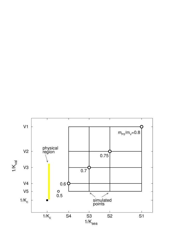
FIG. 1.: Schematic plot for the choice of sea and valence hopping parameters. For circles at the points $\kappa_{\rm val}=\kappa_{\rm sea}$ the corresponding pseudoscalar to vector meson mass ratio is indicated.

FIG. 2.: Effective mass plots for pseudoscalar, vector, nucleon and $\Delta$ channels with degenerate valence hopping parameters $\kappa_{\rm val}=\kappa_{\rm sea}=0.1445$ at $\beta=1.8$. Circles represent effective masses obtained when all quark propagators are calculated with point sources. For squares all quark propagators have smeared sources and triangles are for mixed combinations of sources. Solid lines denote the results from correlated mass fits to smeared source hadron propagators. Dashed lines show the one standard deviation error band determined by jack-knife analysis with a bin size of 10 configurations.

FIG. 3.: Effective mass plots for pseudoscalar, vector, nucleon and $\Delta$ channels with degenerate valence hopping parameters $\kappa_{\rm val}=\kappa_{\rm sea}=0.1400$ at $\beta=1.95$. Symbols have the same meaning as in Fig. 2.

FIG. 4.: Effective mass plots for pseudoscalar, vector, nucleon and $\Delta$ channels with degenerate valence hopping parameters $\kappa_{\rm val}=\kappa_{\rm sea}=0.1374$ at $\beta=2.1$. Symbols have the same meaning as in Fig. 2.

FIG. 5.: Effective mass plots of potential data at $r=L/4$ for sea quark mass corresponding to $m_{\rm PS}/m_{\rm V}\approx 0.7$. The scale is fixed from $\rho$ meson mass at the physical point.

FIG. 6.: Static quark potential on $24^{3}\times 48$ lattice at $\kappa_{\rm sea}=$ 0.1374. Both vertical and horizontal lines are normalized by the Sommer scale $r_{0}$. The solid line represents the fit curve of Eq. (29).

FIG. 7.: Two examples of autocorrelation function (lower symbols) and cumulative autocorrelation time (upper symbols) for $N_{\rm inv}$. Errors are determined with the jack-knife method. Also plotted are two lines $y(t)=t/4$ and $y(t)=t/10$ within which a plateau of $\tau^{\rm cum}(t)$ can be observed.

     

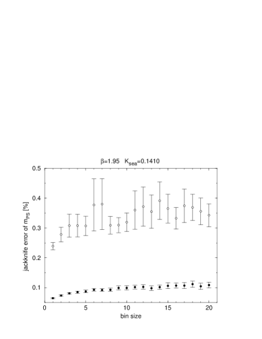
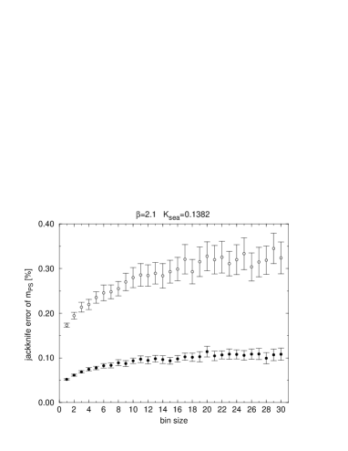
FIG. 8.: Relative errors of the pseudoscalar meson mass as a function of the bin size. Two examples are shown, each at the lightest sea quark mass of $m_{\rm PS}/m_{\rm V}\approx 0.6$. Data at the heaviest valence quark mass are represented by filled symbols and the ones from the lightest valence quark mass with open symbols.

     

     

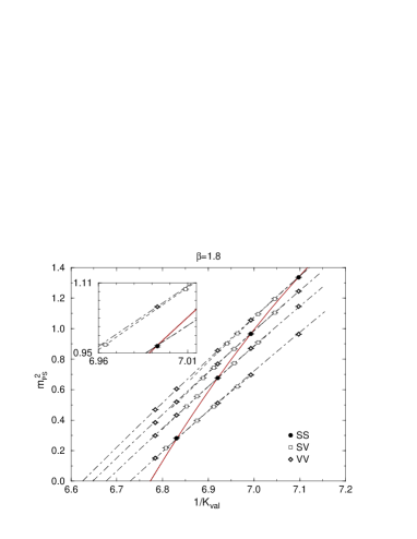
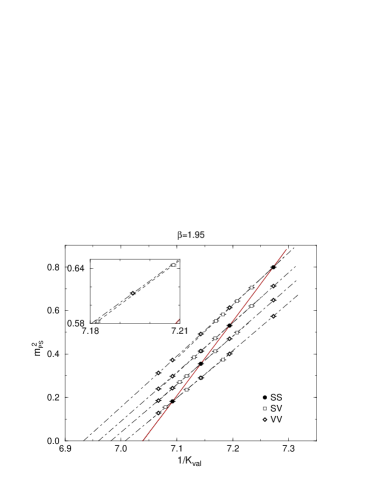
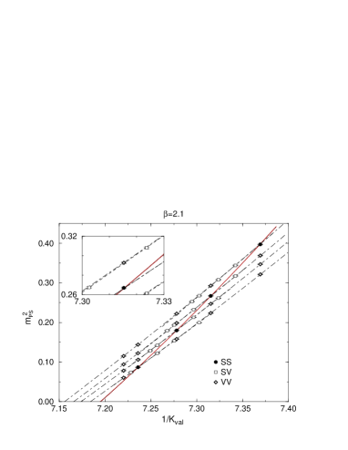
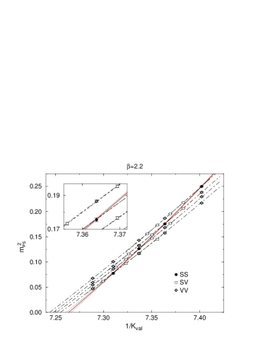
FIG. 9.: Chiral extrapolations of pseudoscalar meson masses. S and V are for valence quarks equal or different to the sea quark. Lines are from combined quadratic fits with Eq. (41).

     

     

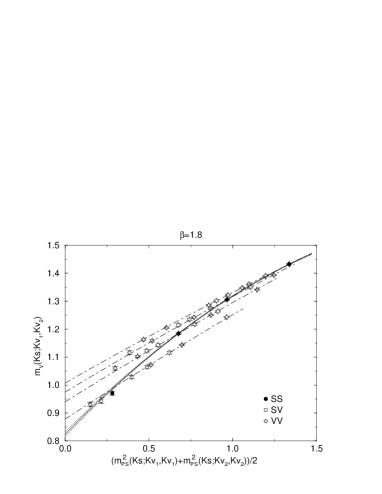
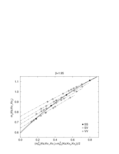
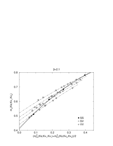
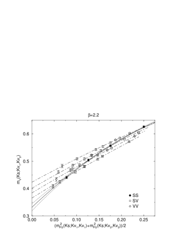
FIG. 10.: Chiral extrapolations of vector meson masses. Lines are from fits with Eq. (49).

     

     

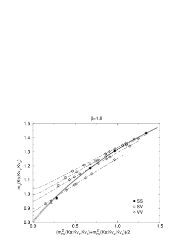
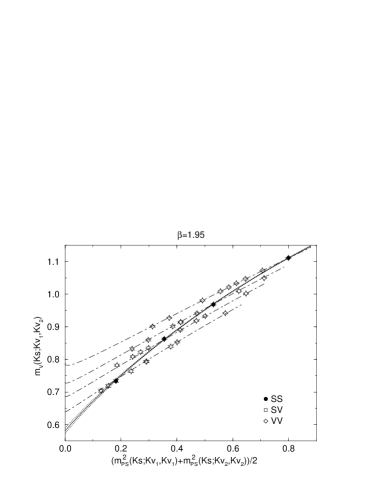
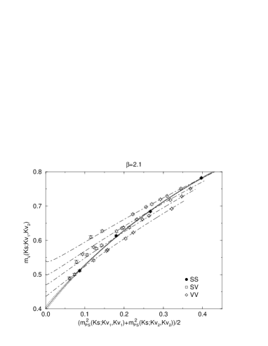
FIG. 11.: Chiral extrapolations of vector meson masses. Mass data are the same as in Fig. 10 but fit lines are from the alternative fits with Eq. (50).

     

     

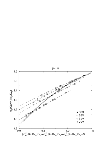
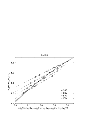
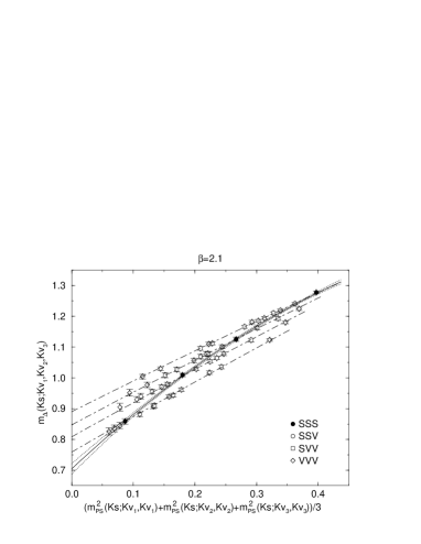
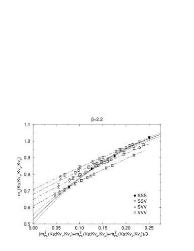
FIG. 12.: Chiral extrapolations of decuplet baryon masses. Lines are from fits with Eq. (52).

     

     

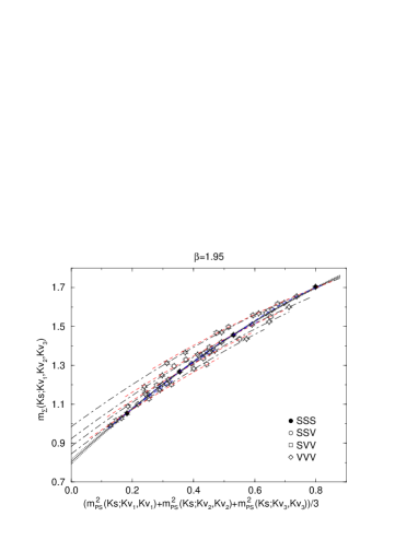
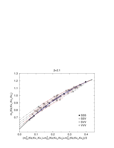
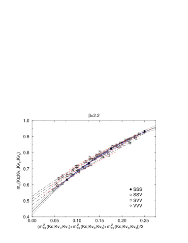
FIG. 13.: Chiral extrapolations of octet baryon masses. Plots only show $\Sigma$-like octet baryons. Lines are from fits with Eq. (55).

     

FIG. 14.: Chiral extrapolations of string tension and Sommer scale.

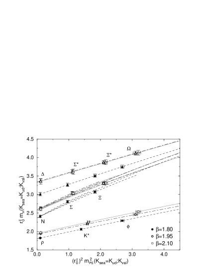
FIG. 15.: Partially quenched spectrum at the physical sea quark mass. Lines are obtained from Eqs. (49), (52) and (55) by fixing $\mu_{\rm sea}=m_{\pi}^{2}$. The strange spectrum, marked with symbols on the lines, is obtained using $M_{K}$ as input.

     

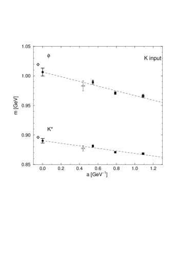
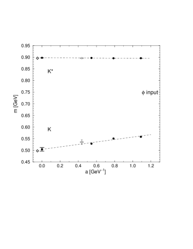
FIG. 16.: Meson masses in full QCD as function of the lattice spacing. Masses in the left hand figures have been obtained using the $K$ meson mass as input while the ones in the right hand figure have been determined using the mass of the $\phi$ meson as input. Experimental values are indicated with diamonds. Masses from the additional run at $\beta=2.2$ are shown with open symbols. Continuum values and extrapolation lines are from a linear fit to the main data at three lattice spacings.

     

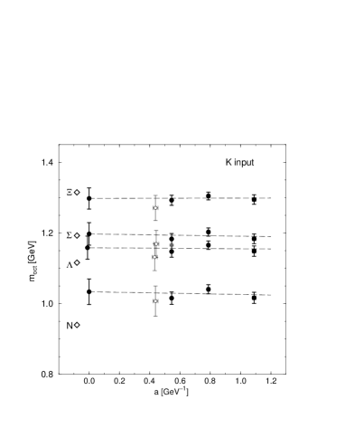
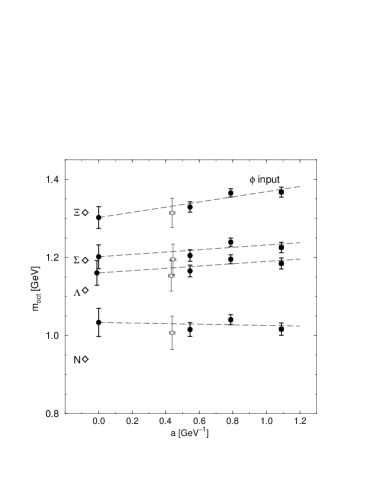
FIG. 17.: Full QCD octet baryon masses as function of the lattice spacing. The strange spectrum is determined with $K$ input (left figure) or $\phi$ input (right figure). Data represented with open symbols are from the run at $\beta=2.2$.

     

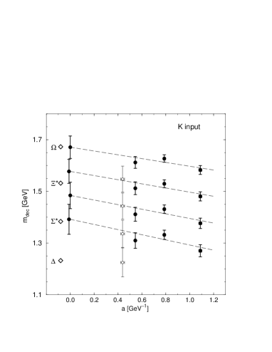
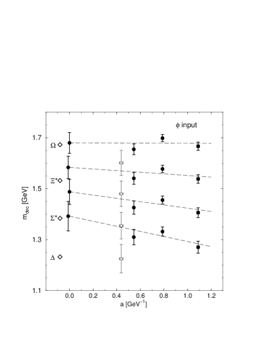
FIG. 18.: Full QCD decuplet baryon masses as function of the lattice spacing. The strange spectrum is determined with $K$ input (left figure) or $\phi$ input (right figure). Data represented with open symbols are from the run at $\beta=2.2$.

FIG. 19.: Chiral extrapolations of vector meson masses in quenched QCD. Lines are from linear fits with Eq. (65).

FIG. 20.: Chiral extrapolations of octet baryon masses in quenched QCD. While fits have been made to $\Sigma$ and $\Lambda$ type baryons of all degeneracies together, only data and lines for degenerate masses are plotted for the sake of clarity.

FIG. 21.: Chiral extrapolations of decuplet baryon masses in quenched QCD. Lines are from linear fits as described in the text.

     

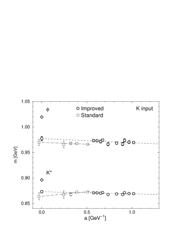
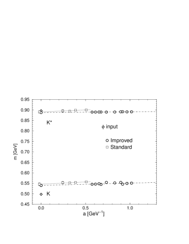
FIG. 22.: Meson masses in quenched QCD with improved and standard actions.

     

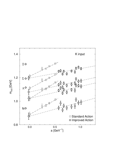
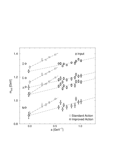
FIG. 23.: Octet baryon masses in quenched QCD with improved and standard actions. The strange spectrum is determined with $K$ input (left figure) or $\phi$ input (right figure).

     

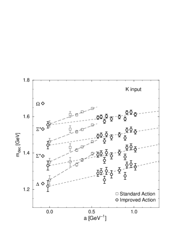
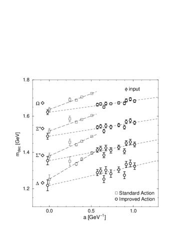
FIG. 24.: Decuplet baryon masses in quenched QCD with improved and standard actions. The strange spectrum is determined with $K$ input (left figure) or $\phi$ input (right figure).

     

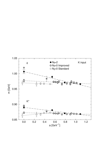
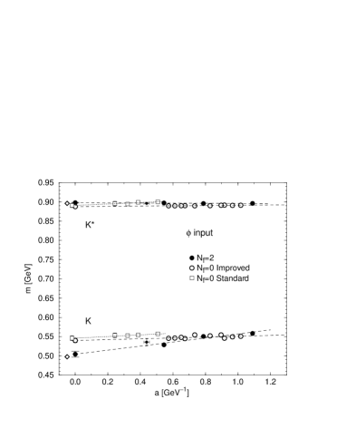
FIG. 25.: Comparison of meson masses in full and quenched QCD. Data from the additional full QCD run at $\beta=2.2$ are shown with small filled circles.

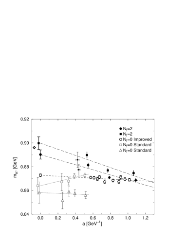
FIG. 26.: Influence of choice of functional form for chiral extrapolation on the $K^{*}$ mass. Filled symbols are for full QCD where for chiral extrapolations Eq.(49) (circles) or Eq.(50) (squares) are used. Data at $\beta=2.2$ are shown with small filled symbols. Masses in quenched QCD with the standard action are shown with open squares for polynomial chiral fits or with open triangles for fits based on quenched chiral perturbation theory.

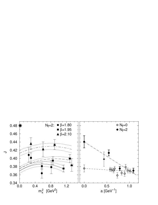
FIG. 27.: The parameter $J$ in full QCD (left figure) as a function of the sea pion mass and as a function of the lattice spacing in quenched and full QCD (right figure). Individual points in the left figure are from separate partially quenched fits while lines are from combined fits. The star denotes the experimental value. Points for full QCD in the right figure are at the physical pion mass.

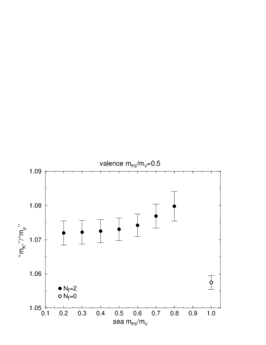
FIG. 28.: Sea quark mass dependence of fictitious mass ratio “$m_{K^{*}}$”$/$“$m_{\rho}$” in the continuum limit.

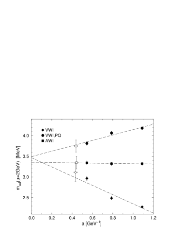
FIG. 29.: Average up and down quark mass for three different definitions in full QCD. Lines are from linear extrapolations to the continuum limit made separately for each definition.

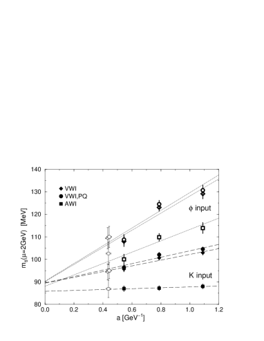
FIG. 30.: Strange quark mass for three different definitions and two different experimental inputs in full QCD. Lines are from linear extrapolations to the continuum limit made separately for each definition.

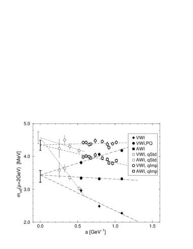
FIG. 31.: Comparison of average up and down quark mass in quenched and full QCD. Lines are from combined linear continuum extrapolations as described in the text.

     

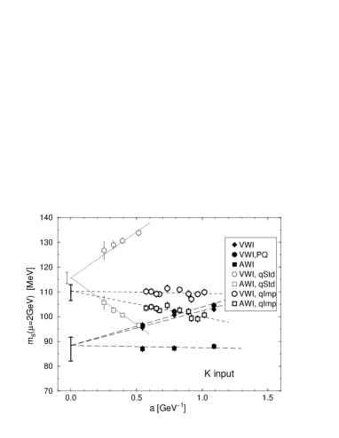
FIG. 32.: Comparison of strange quark mass in quenched and full QCD using as experimental input the $K$ meson mass (left figure) or the $\phi$ meson mass (right figure). Lines are from combined linear continuum extrapolations as described in the text.

     

     

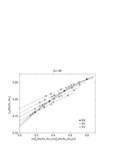
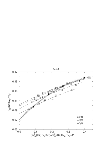
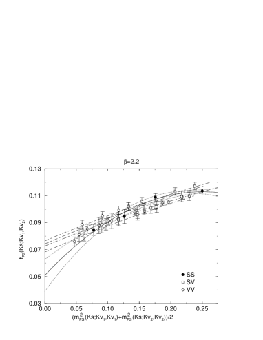
FIG. 33.: Chiral extrapolations of pseudoscalar decay constants. Lines are from fits with Eq. (79).

FIG. 34.: Chiral extrapolations of pseudoscalar decay constants in quenched QCD.

     

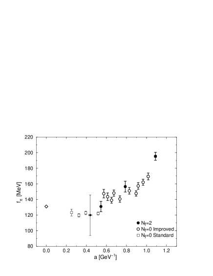
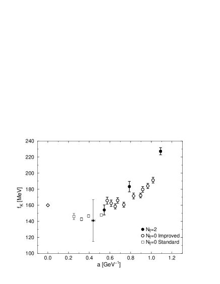
FIG. 35.: Lattice spacing dependence of pseudoscalar decay constants $f_{\pi}$ and $f_{K}$ in full QCD (filled circles) and quenched QCD with improved actions (large open circles) or standard action (small open squares). The strange quark mass used in the calculation of $f_{K}$ is fixed with the $K$ meson mass as input.

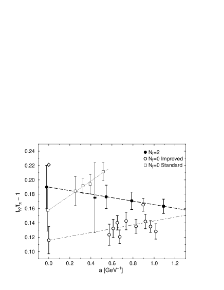
FIG. 36.: Comparison of $f_{K}/f_{\pi}-1$ in full and quenched QCD. Fit lines are linear for all data.

     

     

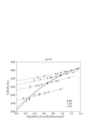
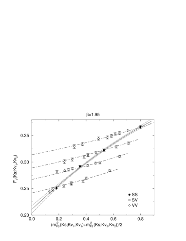
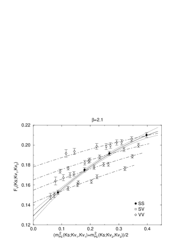
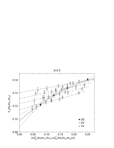
FIG. 37.: Chiral extrapolations of vector meson decay constants. Lines are from fits with Eq. (79).

FIG. 38.: Chiral extrapolation of vector meson decay constants in quenched QCD.

     

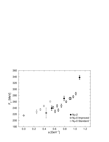
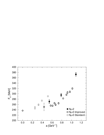
FIG. 39.: Lattice spacing dependence of decay constants $F_{\rho}$ and $F_{\phi}$ in full and quenched QCD.

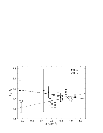
FIG. 40.: Ratio of pseudoscalar and vector decay constants in full and quenched QCD.

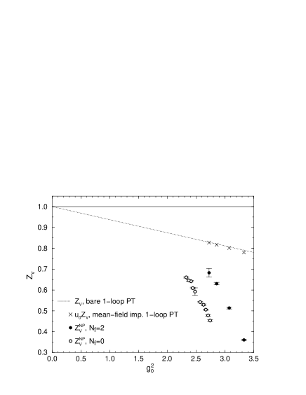
FIG. 41.: Perturbative and non-perturbative $Z$-factors for vector current at zero quark mass.

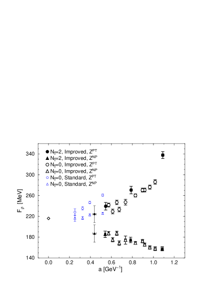
FIG. 42.: Comparison of $F_{\rho}$ in full and quenched QCD with perturbative (circles) and non-perturbative $Z$ factors (triangles).

REFERENCES

- [1] K. G. Wilson, Phys. Rev. D 10, 2445 (1974).
- [2] S. Weinberg, Trans. N.Y. Acad. Sci. 38, 185 (1977).
- [3] H. Hamber and G. Parisi, Phys. Rev. Lett. 47, 1792 (1981); D. Weingarten, Phys. Lett. B 109, 57 (1982).
- [4] F. Butler, H. Chen, J. Sexton, A. Vaccarino and D. Weingarten, Nucl. Phys. B430, 179 (1994).
- [5] CP-PACS Collaboration, S. Aoki et al., Phys. Rev. Lett. 84, 238 (2000).
- [6] M. Fukugita, Y. Oyanagi and A. Ukawa, Phys. Rev. Lett. 57, 953 (1986); Phys. Rev. D 36, 824 (1987).
- [7] R. Gupta, A. Patel, C. F. Baillie, G. Guralnik, G. W. Kilcup and S. R. Sharpe, Phys. Rev. D 40, 2072 (1989).
- [8] K. M. Bitar et al., Phys. Rev. D 42, 3794 (1990); ibid. 46, 2169 (1992).
- [9] F. R. Brown et al., Phys. Rev. Lett. 67, 1062 (1991).
- [10] R. Gupta, C. F. Baillie, R. G. Brickner, G. W. Kilcup, A. Patel and S. R. Sharpe, Phys. Rev. D 44, 3272 (1991).
- [11] M. Fukugita, N. Ishizuka, H. Mino, M. Okawa and A. Ukawa, Phys. Rev. Lett. 68, 761 (1992); Phys. Rev. D 47, 4739 (1993).
- [12] MILC Collaboration, C. Bernard et al., Phys. Rev. D 48, 4419 (1993); S. Gottlieb, Nucl. Phys. B (Proc. Suppl.) 53, 155 (1997).
- [13] K. M. Bitar et al., Phys. Rev. D 49, 3546 (1994).
- [14] K. M. Bitar, R. G. Edwards, U. M. Heller and A. D. Kennedy, Nucl. Phys. B (Proc. Suppl.) 53, 225 (1997).
- [15] MILC Collaboration, C. Bernard et al., Nucl. Phys. B (Proc. Suppl.) 73, 198 (1999) and references cited therein.
- [16] SESAM Collaboration, N. Eicker et al., Phys. Rev. D 59, 014509 (1999).
- [17] UKQCD Collaboration, C.R. Allton et al., Phys. Rev. D 60, 034507 (1999).
- [18] QCDSF and UKQCD Collaborations, H. Stüben et al., Nucl. Phys. B (Proc. Suppl.) 94, 273 (2001).
- [19] Y. Iwasaki, Nucl. Phys. B (Proc. Suppl.) 60A, 246 (1998).
- [20] K. Nakazawa, H. Nakamura, T. Boku, I. Nakata, Y. Yamashita, Parallel Computing 25, 1635 (1999).
- [21] CP-PACS Collaboration, S. Aoki et al., Nucl. Phys. B (Proc. Suppl.) 73, 192 (1999); 73, 216 (1999); R. Burkhalter, ibid. 73 3 (1999); CP-PACS Collaboration, A. Ali Khan et al., ibid. 83, 176 (2000); 94, 229 (2001).
- [22] CP-PACS Collaboration, S. Aoki et al., Phys. Rev. D 60, 114508 (1999).
- [23] Y. Iwasaki, Nucl. Phys. B258, 141 (1985); Univ. of Tsukuba report UTHEP-118 (1983), unpublished.
- [24] B. Sheikholeslami and R. Wohlert, Nucl. Phys. B259, 572 (1985).
- [25] B. J. Gough et al., Phys. Rev. Lett. 79, 1622 (1997).
- [26] JLQCD Collaboration, S. Aoki et al., Phys. Rev. Lett. 82, 4392 (1999).
- [27] J. Garden, J. Heitger, R. Sommer and H. Wittig, Nucl. Phys. B571, 237 (2000).
- [28] M. Göckeler et al., Phys. Rev. D 62, 054504 (2000).
- [29] SESAM Collaboration, N. Eicker et al., Phys. Lett. B 407, 290 (1997).
- [30] CP-PACS Collaboration, A. Ali Khan et al., Phys. Rev. Lett. 85, 4674 (2000).
- [31] CP-PACS Collaboration, A. Ali Khan et al., Nucl. Phys. B (Proc. Suppl.) 83, 162 (2000).
- [32] CP-PACS Collaboration, A. Ali Khan et al., hep-lat/0010009.
- [33] CP-PACS Collaboration, A. Ali Khan et al., hep-lat/0103020.
- [34] CP-PACS Collaboration, T. Manke et al., Phys. Rev. D 62, 114508 (2000); hep-lat/0103015.
- [35] S. Aoki, R. Frezzotti and P. Weisz, Nucl. Phys. B540, 501 (1999).
- [36] H. van der Vorst, SIAM (Soc. Ind. Appl. Math.) J. Sci. Stat. Comput. 13, 631 (1992).
- [37] A. Frommer, V. Hannemann, B. Nöckel, T. Lippert and K. Schilling, Int. J. Mod. Phys. C 5, 1073 (1994).
- [38] J. C. Sexton and D. H. Weingarten, Nucl. Phys. B380, 665 (1992).
- [39] S. Aoki, R. Burkhalter, K. Kanaya, T. Yoshié, T. Boku, H. Nakamura and Y. Yamashita, Parallel Computing 25, 1243 (1999).
- [40] JLQCD Collaboration, S. Aoki et al., Phys. Rev. Lett. 80, 5711 (1998).
- [41] M. Bochicchio, L. Maiani, G. Martinelli, G. C. Rossi and M. Testa, Nucl. Phys. B262, 331 (1985).
- [42] S. Itoh, Y. Iwasaki, Y. Oyanagi and T. Yoshié, Nucl. Phys. B274, 33 (1986).
- [43] G. S. Bali and K. Schilling, Phys. Rev. D 46, 2636 (1992); G. S. Bali, K. Schilling and C. Schlichter, ibid. 51, 5165 (1995).
- [44] C. B. Lang and C. Rebbi, Phys. Lett. B 115, 137 (1982).
- [45] R. Sommer, Nucl. Phys. B411, 839 (1994).
- [46] N. Madras and A. D. Sokal, J. Statist. Phys. 50, 109 (1988).
- [47] SESAM Collaboration, T. Lippert et al., Nucl. Phys. B (Proc. Suppl.) 63, 946 (1998).
- [48] E. Jenkins, A. V. Manohar and M. B. Wise, Phys. Rev. Lett. 75, 2272 (1995).
- [49] M. Golterman, private communication.
- [50] V. Bernard, N. Kaiser and U. G. Meissner, Z. Phys. C 60, 111 (1993).
- [51] S. Aoki, Nucl. Phys. B (Proc. Suppl.) 94, 3 (2001).
- [52] P. Lacock and C. Michael, Phys. Rev. D 52, 5213 (1995).
- [53] T. Bhattacharya and R. Gupta, Nucl. Phys. B (Proc. Suppl.) 63, 95 (1998).
- [54] L. Maiani and G. Martinelli, Phys. Lett. B 178, 265 (1986).
- [55] R. Lewis and R. M. Woloshyn, Phys. Rev. D 56, 1571 (1997).
- [56] G. Martinelli and C. T. Sachrajda, Nucl. Phys. B316, 355 (1989).
- [57] S. Aoki, K. Nagai, Y. Taniguchi and A. Ukawa, Phys. Rev. D 58, 074505 (1998); Y. Taniguchi and A. Ukawa, ibid. 58, 114503 (1998).
- [58] G. P. Lepage and P. B. Mackenzie, Phys. Rev. D 48, 2250 (1993).