NTUA- 4/01

Multi–Layer Structure
in the Strongly Coupled 5D Abelian Higgs Model

P. Dimopoulos^(a), K. Farakos^(a), and S. Nicolis^(b)

^(a) Physics Department, National Technical University
15780 Zografou Campus, Athens, Greece

^(b) CNRS-Laboratoire de Mathématiques et Physique Théorique (UMR 6083)
Université de Tours, Parc Grandmont, 37200 Tours,France

We explore the phase diagram of the five-dimensional anisotropic Abelian Higgs model by Monte Carlo simulations. In particular, we study the transition between the confining phase and the four dimensional layered Higgs phase. We find that, in a certain region of the lattice parameter space, this transition can be first order and that each layer moves into the Higgs phase independently of the others ( decoupling of layers). As the Higgs couplings vary, we find, using mean field techniques, that this transition may probably become second order.

1 Introduction

Coupling anisotropies in gauge theories may lead to fundamental changes in their phase diagrams. Although this yields problematic theories if applied to four-dimensional models, due to breakdown of Lorentz invariance, higher-dimensional models with anisotropic couplings may give rise to theories of physical interest. This programme originated in 1984 by Fu and Nielsen [1] who considered a five-dimensional pure U(1) gauge theory on the lattice. The main idea is that, for certain values of the couplings for the $n$ extra dimensions, four-dimensional layers may be formed within the $(4+n)-$dimensional space. The corresponding phase is called layered phase and one of its main characteristics is that exhibits confinement in the extra dimensions. The U(1) higher-dimensional model has already been studied to some extent with lattice techniques ([2], [3]), leading to the establishment of the existence of a layered Coulomb phase.

The possibility that physical space–time is not four-dimensional has been broadly referred to in the bibliography during the last eighty years. This interesting idea has enjoyed a revival through works that use extra dimensions to solve the hierarchy problem. A class of these theories use a (4+n)-dimensional space–time with n compactified dimensions; another class of models considers non–compact extra dimensions. A well–known example of this last case is the Randall–Sundrum (RS) model [5], where the four-dimensional world is considered as a three–brane embedded in a five-dimensional bulk. Furthermore in such models a four–dimensional graviton exists and is localised within the three-brane. The question which then arises is if there is any possibility that other fields, such as gauge fields, fermions and scalars are localised within a 3-brane. The problem has been attacked analytically through the search for localized four–dimensional fields, where the equations of motion of the bulk fields which are coupled to the background geometry are solved [6]. In this approach, using perturbative tools, a massless photon always appears propagating freely in five dimensions. A first attempt of getting evidence of gauge field localization on a brane considering the non–perturbative features while using an RS action type for abelian gauge field has been performed in [3] by means of lattice techniques.

Theories on flat spacetimes are not, however, devoid of interest. In this paper we continue to explore the phase structure of the Abelian Higgs model in five dimensions with anisotropic couplings, defining our model on the lattice. In a previous paper[7] we studied the phase diagram of this model for weak gauge coupling in the four-dimensional subspace and found two kinds of layers (or 3-branes): of Coulomb or Higgs type. In the present paper we wish to explore the strongly coupled theory, motivated, in part, by recent considerations that indicate that theories studied in ref. [6] are, generically, strongly coupled.

We find that it is, indeed, possible to tune the lattice couplings in such a way that a phase transition from the five-dimensional strong phase to a layered phase occurs. By measuring several order parameters we find that the layers are in the Higgs phase and they are separated from each other by a confining force. Furthermore we show the precise way in which they are created by studying in detail the phase transition. In particular, we find that each layer emerges from the confining phase independently from the others-characteristic of a strongly first order phase transition with a very small correlation length in the extra direction.

In section 2 we write down the Abelian Higgs model in five dimensions with anisotropic couplings. In section 3 we present the Monte–Carlo results, we exhibit the phase structure and we establish the existence of the layered Higgs phase. Also, using mean field techniques, we confirm the Monte–Carlo results and we give indication of how the situation changes as we vary the Higgs lattice couplings.

2 Formulation of the model

The model under study is the Abelian Higgs model in the five-dimensional space. Direction $\hat{5}$ will be singled out by couplings that will differ from the corresponding ones in the remaining four directions.

We proceed with writing down the lattice action of the model.

$$S= \beta_{g} \sum_{x}\sum_{1\leq\mu<\nu\leq 4}(1-\cos F_{\mu\nu}(x))+\beta_{g}^{\prime}\sum_{x}\sum_{1\leq\mu\leq 4}(1-\cos F_{\mu 5}(x))$$ (1)

$$+ \beta_{h}\sum_{x}{\rm Re}[4\varphi^{*}(x)\varphi(x)-\sum_{1\leq\mu\leq 4}\varphi^{*}(x)U_{\hat{\mu}}(x)\varphi(x+\hat{\mu})]$$

$$+ \beta_{h}^{\prime}\sum_{x}{\rm Re}[\varphi^{*}(x)\varphi(x)-\varphi^{*}(x)U_{\hat{5}}(x)\varphi(x+\hat{5})]$$

$$+ \sum_{x}[(1-2\beta_{R}-4\beta_{h}-\beta_{h}^{\prime})\varphi^{*}(x)\varphi(x)+\beta_{R}(\varphi^{*}(x)\varphi(x))^{2}],$$

where

$$F_{\mu\nu}(x)=A_{\mu}(x)+A_{\nu}(x+\hat{\mu})-A_{\mu}(x+\hat{\nu})-A_{\nu}(x),~{}~{}1\leq\mu<\nu\leq 4,$$

$$F_{\mu 5}(x)=A_{\mu}(x)+A_{5}(x+\hat{\mu})-A_{\mu}(x+\hat{5})-A_{5}(x)~{}~{}1\leq\mu\leq 4.$$

We have allowed for different couplings in the various directions: the ones pertaining to the fifth direction are primed to distinguish them from the “space-like” couplings. The fifth direction will also be called “transverse” in the sequel.

The link variables $U_{\hat{\mu}}(x)$ are defined as $e^{i\alpha_{S}{\overline{A}_{S}}}$ or $e^{i\alpha_{T}{\overline{A}_{T}}}$ respectively, where ${\overline{A}_{S}},~{}~{}{\overline{A}_{T}}$ are the continuum fields and $\alpha_{S},~{}\alpha_{T}$ are the lattice spacings in the space-like and the transverse-like dimensions respectively. The lattice fields are

$$A_{S}\equiv\alpha_{S}{\overline{A}_{S}},~{}~{}A_{T}\equiv\alpha_{T}{\overline{A}_{T}}.$$

In addition, the scalar fields are also written in the polar form $\varphi(x)=\rho(x)e^{i\chi(x)}.$ The order parameters that we will use are the following:

$${\rm Space-like~{}Plaquette:~{}~{}~{}}P_{S}\equiv<\frac{1}{6N^{5}}\sum_{x}\sum_{1\leq\mu<\nu\leq 4}\cos F_{\mu\nu}(x)>$$ (2)

$${\rm Transverse-like~{}Plaquette:~{}~{}~{}}P_{T}\equiv<\frac{1}{4N^{5}}\sum_{x}\sum_{1\leq\mu\leq 4}\cos F_{\mu 5}(x)>$$ (3)

$${\rm Space-like~{}Link:~{}~{}~{}}L_{S}\equiv<\frac{1}{4N^{5}}\sum_{x}\sum_{1\leq\mu\leq 4}\cos(\chi(x+\hat{\mu})+A_{\hat{\mu}}(x)-\chi(x))>$$ (4)

$${\rm Transverse-like~{}Link:~{}~{}~{}}L_{T}\equiv<\frac{1}{N^{5}}\sum_{x}\cos(\chi(x+\hat{5})+A_{\hat{5}}(x)-\chi(x))>$$ (5)

$${\rm Higgs~{}field~{}measure~{}squared:~{}~{}~{}}R^{2}\equiv\frac{1}{N^{5}}\sum_{x}\rho^{2}(x)$$ (6)

In the above equations $N$ is the linear dimension of a symmetric $N^{5}$ lattice.

When necessary we will use the order parameters $L_{S}$ and $P_{S}$ defined on each space–like volume (layer) separately.

The naïve continuum limit of the lattice action 1 may be obtained as follows (where an overbar is used for the continuum fields):

$$\varphi={\overline{\varphi}}\sqrt{\frac{2a_{S}^{2}a_{T}}{\beta_{h}}},$$

$$~{}~{}A_{\mu}=a_{S}{\overline{A}_{\mu}},~{}~{}1\leq\mu\leq 4,$$

$$~{}~{}A_{5}=a_{T}{\overline{A}_{5}}.$$

Then the transverse-like field strength

$$F_{\mu 5}\equiv A_{\mu}(x)+A_{5}(x+\hat{\mu})-A_{\mu}(x+\hat{5})-A_{5}(x)~{}~{}(1\leq\mu\leq 4)$$

goes over to:

$$-a_{S}[a_{T}\partial_{5}{\overline{A}_{\mu}}(x)]+a_{T}[a_{S}\partial_{\mu}{\overline{A}_{5}}(x)]=a_{S}a_{T}(\partial_{\mu}{\overline{A}_{5}}-\partial_{5}{\overline{A}_{\mu}}).$$

Thus

$$F_{\mu 5}^{2}\rightarrow a_{S}^{2}a_{T}^{2}{\overline{F}_{\mu 5}^{2}},~{}~{}1\leq\mu\leq 4~{}~{}(F_{\mu 5}\equiv\partial_{\mu}{\overline{A}_{5}}-\partial_{5}{\overline{A}_{\mu}}).$$

The space-like field strength is treated in a very similar way with the result:

$$F_{\mu\nu}^{2}\rightarrow a_{S}^{4}{\overline{F}_{\mu\nu}^{2}},~{}~{}{\overline{F}_{\mu\nu}}\equiv\partial_{\mu}{\overline{A}_{\nu}}-\partial_{\nu}{\overline{A}_{\mu}},~{}~{}1\leq\mu<\nu\leq 4.$$

This means that the transverse-like part of the pure gauge action is rewritten in the form:

$$\frac{1}{2}\frac{{\beta_{g}}^{\prime}a_{T}}{a_{S}^{2}}\sum a_{S}^{4}a_{T}[\sum_{1\leq\mu\leq 4}{\overline{F}}_{\mu 5}^{2}]\rightarrow\frac{1}{2}\frac{{\beta_{g}}^{\prime}a_{T}}{a_{S}^{2}}\int d^{5}x[\sum_{1\leq\mu\leq 4}{\overline{F}}_{\mu 5}^{2}].$$

On the other hand the space–like part is:

$$\frac{1}{2}\frac{\beta_{g}}{a_{T}}\sum a_{S}^{4}a_{T}[\sum_{1\leq\mu<\nu\leq 4}{\overline{F}}_{\mu\nu}^{2}]\rightarrow\frac{1}{2}\frac{\beta_{g}}{a_{T}}\int d^{5}x[\sum_{1\leq\mu<\nu\leq 4}{\overline{F}}_{\mu\nu}^{2}].$$

If we define

$$\beta_{g}\equiv\frac{a_{T}}{g_{S}^{2}},~{}~{}{\beta_{g}}^{\prime}\equiv\frac{a_{S}^{2}}{g_{T}^{2}a_{T}},$$ (7)

the resulting continuum action reads:

$$\frac{1}{2}\int d^{5}x\left[\frac{1}{g_{S}^{2}}\sum_{1\leq\mu<\nu\leq 4}{\overline{F}_{\mu\nu}}^{2}+\frac{1}{g_{T}^{2}}\sum_{1\leq\mu\leq 4}{\overline{F}_{\mu 5}}^{2}\right]$$

Defining $\gamma_{g}\equiv(\frac{{\beta_{g}}^{\prime}}{\beta_{g}})^{1/2}$ and using the definitions of $\beta_{g}$, ${\beta_{g}}^{\prime}$ we find that

$$\gamma_{g}=\frac{g_{S}}{g_{T}}\frac{a_{S}}{a_{T}}.$$

We denote by $\xi$ the important ratio $\frac{a_{S}}{a_{T}}$ of the two lattice spacings (the correlation anisotropy parameter) and finally derive the relation:

$$\gamma_{g}=\sqrt{\frac{{\beta_{g}}^{\prime}}{\beta_{g}}}=\frac{g_{S}}{g_{T}}\xi.$$

After rescaling the scalar fields, one may rewrite the scalar sector of the action in the form:

$$\int d^{5}x[\sum_{1\leq\mu\leq 4}|D_{\mu}{\overline{\varphi}}|^{2}+\frac{\gamma_{\varphi}^{2}}{\xi^{2}}|D_{5}{\overline{\varphi}}|^{2}+m^{2}{\overline{\varphi}}^{*}{\overline{\varphi}}+\lambda({\overline{\varphi}}^{*}{\overline{\varphi}})^{2}],$$ (8)

where $D_{\mu}\equiv\partial_{\mu}-i{\overline{A}_{\mu}},~{}~{}1\leq\mu\leq 5.$

We have used the notations:

$$\gamma_{\varphi}\equiv\sqrt{\frac{{\beta_{h}}^{\prime}}{\beta_{h}}},$$

$$m^{2}a{{}_{S}}^{2}\equiv\frac{2}{\beta_{h}}(1-2\beta_{R}-4\beta_{h}-{\beta_{h}}^{\prime}),~{}~{}\frac{\lambda}{a_{S}}=\frac{4\beta_{R}}{\beta_{h}^{2}\xi}.$$

If we choose a common value for the gauge coupling constants: $g_{S}=g_{T}\equiv g,$ (so that $\gamma_{g}=\xi,$) and assume that all the covariant derivatives in equation (8) have the same factor in front: $\gamma_{\phi}=\xi$, the expression does not exhibit any anisotropy. However, the naïveté of this approach will be manifest by results similar to Ref. [2, 3, 7] which indicate that the anisotropy may survive in the continuum limit for a wide range of values of lattice parameters both in flat as well as in warped (Randall-Sundrum type) spacetimes.

3 Monte Carlo Results
and the Confining–Layered Transition

For the simulations we use 5-hit Metropolis algotithm for the updating of both the gauge and Higgs fields. In order to get better behaviour we use a global radial algorithm and an overrelaxation algorithm for the updating of the Higgs field. We simulated the system for $4^{5},6^{5},\mbox{and}\hskip 2.84544pt8^{5}$ lattices. We made use, mainly, of the hysteresis loop method to establish the phase diagram of the system. When necessary, in order to define more precisely the phase transition points and study the order of the phase transition we made long runs consisting up to 30000 measurements at selected points in the parameter space.

In whole work we set the four–dimensional gauge coupling fixed at the value $\beta_{g}=0.5$ and let the gauge coupling in the fifth direction run. For some regions of the values of the two gauge couplings we had a confining five–dimensional theory. A small value for the Higgs coupling constant $\beta_{h}^{\prime}$ in the fifth dimension has been chosen ($\beta_{h}^{\prime}=0.001$) (we further discuss this choice in Section 3.2) and we used two values for the Higgs self–coupling $\beta_{R}$ differing by one order of magnitude: $\beta_{R}=0.01$ and $\beta_{R}=0.1$. Thus the phase diagram has been found in the $\beta_{g}^{\prime}-\beta_{h}$ subspace.

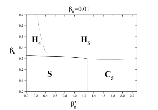
Figure 1: Phase diagram for $\beta_{R}=0.01$

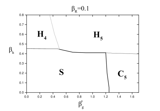
Figure 2: Phase diagram for $\beta_{R}=0.1$

We study the behaviour of the system in terms of the order parameters defined in Section 2. We proceed now with the presentation of the phase structure.

Figures 1 and 2 show the phase diagrams of the 5–dimensional Abelian Higgs model for the cases of two values of $\beta_{R}$ coupling, namely $\beta_{R}=0.01$ and $\beta_{R}=0.1$, respectively. The phase diagram for both cases has been explored in $\beta_{g}^{\prime}-\beta_{h}$ subspace. In Table 1 we show the values for the couplings from which we deduced the phase diagrams.

	$\beta_{R}=0.01$			$\beta_{R}=0.1$
	$\beta_{g}^{\prime}$	$\beta_{h}$	$\beta_{g}^{\prime}$	$\beta_{h}$
$S-H_{4}$	0.05, 0.10, 0.20,		0.10, 0.20, 0.25,
	0.40, 0.45		0.30, 0.40, 0.45, 0.46
$S-H_{5}$	0.50, 0.70, 0.80,		0.47, 0.50, 0.70,
	0.90, 1.00		0.90, 1.00, 1.10
$C_{5}-H_{5}$	1.40, 1.50, 1.90		1.20, 1.30, 1.50
$H_{4}-H_{5}$		0.40, 0.50, 0.60		0.50, 0.60, 0.80
$S-C_{5}$		0.05, 0.15, 0.20,		0.10, 0.20, 0.30
		0.25, 0.30

Table 1: The phase which the phase diagrams given in Figures 1 and 2 are based on.

The two phase diagrams exhibit similar structure. There are four different phases namely the strong phase (S), the Coulomb phase in five dimensions ($C_{5}$) and the Higgs phases in four ($H_{4}$) and five dimensions ($H_{5}$). More details about the nature of the different phase transitions will be given later. The crucial feature, however, is the existence of a phase transition between the strong phase (eg. a confined phase in five dimensions) and the $H_{4}$ phase –a phase of broken U(1) symmetry in four dimensions– which gives rise to a constitution of a layered phase with broken symmetry on each layer. Let us give now some representative results which lead to the identification of the various phases of the model.

$\bullet$   The $\mathbf{S-H_{4}}$ and $\mathbf{S-H_{5}}$ phase transitions

In Figure 3(a) , we present the hysteresis loops concerning the space–like plaquettes, as $\beta_{h}$ runs, for $\beta_{R}=0.01$ and for two values $\beta_{g}^{\prime}=0.2$ and $\beta_{g}^{\prime}=0.7$. In Figure 3 (b) the corresponding results for the transverse–like plaquettes are depicted.

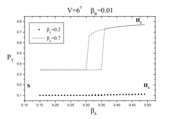
Figure 3: Hysteresis loop for space–like (a) and transverse–like (b) plaquette for two values of $\beta_{g}^{\prime}=0.2$ and 0.7.

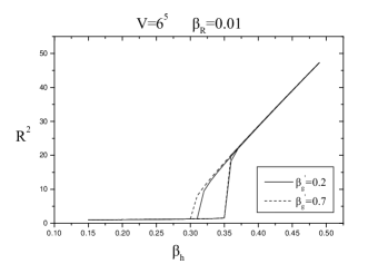
Figure 4: Hysteresis loop for $R^{2}$, $\beta^{\prime}_{g}=0.2,0.7$.

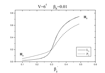
Figure 5: Hysteresis loop analysis for $L_{T}$ and $P_{T}$ in the region between $H_{4}$ and $H_{5}$ phases. The transition is not showing formation of a loop and seems to be fairly smooth.

The behaviour of the space–like plaquettes and also the behaviour of $R^{2}$, shown in Figure 4, lead to the conclusion of a phase transition between the five dimensional strong phase and a phase with broken symmetry which probably is of first order by virtue of the large hysteresis loop. In addition, the transverse–like plaquette, $P_{T}$, for $\beta_{g}^{\prime}=0.2$ remains almost constant to a small value (it equals the value $\beta_{g}^{\prime}/2$, labeling the Strong phase) while the corresponding one for $\beta_{g}^{\prime}=0.7$ increases with $\beta_{h}$ as a phase transition occurs. This is a serious indication that there are two different Higgs phases: in particular one is a Higgs phase in four dimensions (with confining behaviour along the fifth dimension) and the other is a five–dimensional Higgs phase.

$\bullet$   The $\mathbf{H_{4}-H_{5}}$ phase transition

The fact that the fifth dimension is confining is made clearer from the result of Figure 5: we keep $\beta_{h}=0.40$ and let $\beta_{g}^{\prime}$ run. The results depicted in this figure correspond to the values of transverse–like link and transverse–like plaquette which are small enough for small values of $\beta_{g}^{\prime}$ and they increase as this coupling parameter is running to larger values. It can be noticed that there is no obvious hysteresis loop formed and the system passes from the $H_{4}$ (where the two order parameters take small values) to the $H_{5}$ phase in a fairly smooth way.

$\bullet$   The $\mathbf{S-C_{5}}$ and $\mathbf{C_{5}-H_{5}}$ phase transitions

The existence of the $C_{5}$ phase is indicated in Figure 6, which contains the hysteresis loop for $P_{S}$ and $P_{T}$ for running $\beta_{g}^{\prime}$. As it can be easily seen, these two quantities pass from a region where their values are almost half of their corresponding gauge couplings (Strong phase) to a phase ($C_{5}$)where their values tend to one. The large hysteresis loops indicate a first order phase transition for $S-C_{5}$.

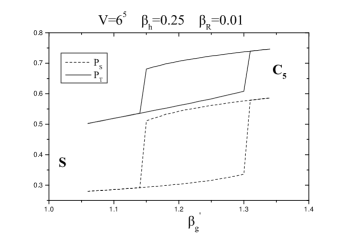
Figure 6: Hysteresis loop for $P_{S}$ and $P_{T}$ for the $S-C_{5}$ phase transition.

Finally, the transition between $C_{5}$ and $H_{5}$ is shown in Figure 7 where we set $\beta_{g}^{\prime}$ to 1.5 and let $\beta_{h}$ run. In Figure 7 (a) we show the behaviour of the space–like and the transverse–like link from which we can see that they both exhibit a gradual increase as $\beta_{h}$ grows. In addition, the corresponding behaviour of $R^{2}$ values in Figure 7 (b) implies the transition from a five–dimensional Coulomb phase to a five–dimensional Higgs phase.

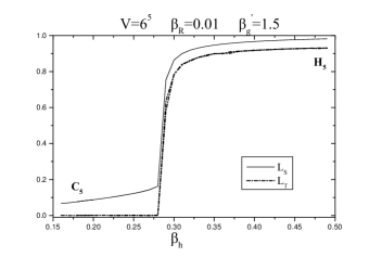
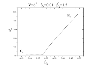
Figure 7: Hysteresis loop for space–like and transverse–like link (a) and $R^{2}$ (b), for $\beta_{g}^{\prime}=1.5$.

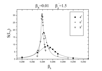
Figure 8: Susceptibility $S(L_{S})$ for three values of lattice volume for $\beta_{g}^{\prime}=1.5$ (the error–bars are smaller than the sizes of the symbols).

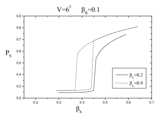
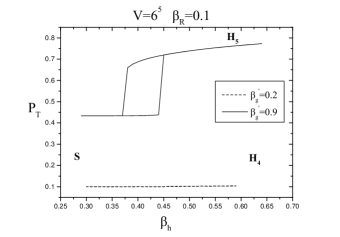
Figure 9: Hysteresis loop for space–like (a) and transverse–like plaquette (b) for $\beta_{g}^{\prime}=0.2$ and $\beta^{\prime}_{g}=0.9$.

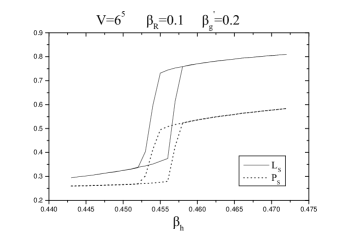
Figure 10: Hysteresis loop for space–like link and plaquette for $\beta_{g}^{\prime}=0.2$ in more detail, indicating a first order phase transition.

The order of the phase transition is not obvious and further study will be needed. To this end we measure the susceptibilities for the $L_{S}$ order parameter at the value $\beta_{g}^{\prime}=1.5$. The results shown in Figure 8 seem to be consistent with a second order phase transition as the maximum values of susceptibility for each volume grows with some power of the volume which is obviously much less than unity.

Up to now, we have given some examples of the behaviour of the system for $\beta_{R}=0.01$. In general, the phase structure for $\beta_{R}$ an order of magnitude larger than this , e.g. $\beta_{R}=0.1$, is similar. However, we can elaborate on some points concerning the structure of the layered phase which is formed in the $S-H_{4}$ transition on one side and the $S-H_{5}$ transition on the other.

In Figure 9 we can see an example for the transition from $S$ to $H_{4}$ ($\beta_{g}^{\prime}=0.2$) and from $S$ to $H_{5}$ ($\beta_{g}^{\prime}=0.9$), by giving the hysteresis loops for $P_{S}$ and $P_{T}$. The difference of this figure with Figure 3 consists in the “weaker” transition from $S$ to $H_{4}$ phase, since the loop is much smaller. A more detailed study for the case $\beta_{g}^{\prime}=0.2$ shows (Figure 10) that a clear hysteresis loop is formed, indicating a first order phase transition, though seemingly weaker, than that of $\beta_{R}=0.01$ case. However, the trasverse–like order parameter $P_{T}$ does not change at all as $\beta_{h}$ increases. This fact points out that a layered phase has appeared and the layers are decoupled from each other.

3.1 Multi–layer Structure

The next step is to study the behaviour of the layers one by one as the system moves through the phase transition. This is shown in Figures 11 (a) and (b) which correspond to $S-H_{4}$ and $S-H_{5}$ phase transitions respectively. In the Figure 11 (a), corresponding to the $S-H_{4}$ case, one may easily see a “non–sychronised” transition exhibited by $L_{S}$ defined on each space–like volume (layer) in contrast with Figure 11 (b), in which the corresponding order parameters indicate the phase transition simultaneously (Obviously, in figure (b) the hysteresis loops formed by the $L_{S}$ defined on each layer can not be distinguished from the corresponding hysteresis loop due to $L_{S}$ defined on the volume.) This specific behaviour of hysteresis loops, may actually serve as a “criterion” to characterise the layered phase.

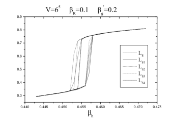
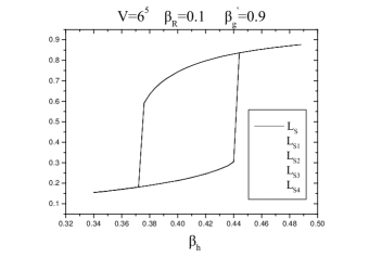
Figure 11: Hysteresis loop for $\beta_{g}^{\prime}=0.2$ (a) and $\beta_{g}^{\prime}=0.9$ (b). We show the very different way for the transition of $L_{S}$ calculated either on the five dimensional volume and on four layers. In the figure on the left the $S-H_{4}$ transition is presented where the layers show a decoherent behaviour on the phase transition in contrast with the $S-H_{5}$ phase transition on the right where the transition for $L_{S}$ is identical for all layers, so it coincides with the mean values over the 5D–volume.

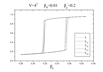
Figure 12: Hysteresis loop for $L_{S}$ showing the way that the layers decouple for $\beta_{R}=0.01$ at $\beta_{g}^{\prime}=0.2$.

We also reach the same conclusion by considering the $\beta_{R}=0.01$, $\beta_{g}^{\prime}=0.2$ case, for a $4^{5}$ lattice in more detail. The result, shown in Figure 12, leads to the same conclusion: The very existence of the layered phase (and consequently of confinement in the fifth dimension) shows up in the “incoherent” behaviour of the space–like volumes (layers) as the phase transition takes place.

This behaviour can be further confirmed by long runs in the transition region. It is to be expected that the $S-H_{4}$ phase transition is of first order. Therefore, we would expect a two peak signal in the order parameter disrtibution at equilibrium. Nevertheless the situation, shown in Figure 13 (a) concerning the distribution for the order parameter $L_{S}$ for a value of $\beta_{h}$ near the transition region for $V=6^{5}$ is by no means what one would expect normally. The multipeak structure seems rather strange. It should be noticed that the same occurs for the order parameter $P_{S}$ too. However, the study of the same order parameter defined on each space–like volume is more illuminating. For example in Figure 13 (b), we can see the distribution of $L_{S}$ values on each layer. We show four out of six distributions of $L_{S}$ corresponding to the four space–like layers within the five–dimensional volume. The distributions which are produced appear quite usual and they show that at the same time one layer is in the strong phase (called $2_{nd}$ in the figure), another has already passed to the broken phase ($3_{rd}$) and others produce a two peak signal result. The result is that the strange picture of the distribution formed in Figure 13 (a) is resolved if we analyze the behaviour of the system on each layer as the system undergoes the phase transition.

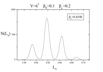
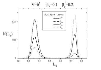
Figure 13: Distribution for $L_{S}$ on the volume (a) and on each layer (only four of the six are shown in the figure)(b) for $6^{5}$ lattice in the critical region for the $S-H_{4}$ phase transition.

This result is found for all of the volume sizes (e.g. $4^{5},6^{5},8^{5}$) which we have worked on. Although it is consistent with a first order phase transition it lends support to the view of a decoherent behaviour for every four–dimensional volume (layer) in the transition region between five–dimensonal strong phase and the four–dimensional layered Higgs phase. This certain behaviour describes a dynamical decoupling of the layers and provides a possible mechanism for localization of the fields on the layers.

3.2 Mean Field Approach

The Mean Field Approach provides a point of view complementary to Monte Carlo sumulations. Although it is, by construction, blind to spatial fluctuations, and cannot, therefore, see the multi-layer structure, it does not suffer from the finite volume effects, that limit Monte Carlo simulations. Furthermore, it is expected to be a reliable guide to the phase diagram, the higher the dimension of the system under study.

Thus, in this work we use the Mean Field analysis (i) to show that the small value of $\beta^{\prime}_{h}$ we have chosen is really a suitable one to reveal the layered Higgs phase and (ii) to provide evidence that as Higgs self–coupling takes larger values –up to $\beta_{R}=0.2$– the phase transition from the Strong to the $H_{4}$ phase may become second order.

We start with the action (1). We fix the gauge by imposing $U_{\hat{4}}(x)=I$ and use the translation-invariant Ansatz [1, 2, 7], $U_{\hat{\mu}}(x)=v,\,1\leq\mu\leq 3$; $U_{\hat{5}}(x)=v^{\prime}$. We also introduce the variables for the Higgs field,

$$\phi(x)=\rho(x)e^{{\mathrm{i}}\chi(x)}$$ (9)

and have also assumed a translationally invariant Ansatz, $\rho=\rho(x)$, $\chi=\chi(x)$. The free energy, which should be minimized to get the mean field solution, reads:

$$F=-\beta_{g}3v_{a}^{4}-\beta_{g}3v_{a}^{2}$$

$$-\beta_{g}^{\prime}3v_{a}^{2}v_{a^{\prime}}^{\prime 2}-\beta_{g}^{\prime}v_{a^{\prime}}^{\prime 2}$$

$$-(3\beta_{h}v_{a}+\beta_{h}+\beta_{h}^{\prime}v_{a^{\prime}}^{\prime})\rho^{2}v_{\chi}^{2}$$

$$+(1-2\beta_{R})\rho^{2}+\beta_{R}\rho^{4}-\frac{1}{2}log[\rho^{2}]$$

$$+3av_{a}-3log[I_{0}(a)]+a^{\prime}v_{a^{\prime}}^{\prime}-log[I_{0}(a^{\prime})]+\chi v_{\chi}-log[I_{0}(\chi)]$$ (10)

The parameters $a$, $a^{\prime}$ and $\chi$ are conjugate to $v_{a}$, $v^{\prime}_{a^{\prime}}$ and $v_{\chi}$ respectively.
We study the phase structure using the order parameters defined in Section 2.

Our Monte Carlo analysis has been performed setting $\beta_{h}^{\prime}=0.001$. It is of interest to have an idea what happens when $\beta_{h}^{\prime}$ takes other values.

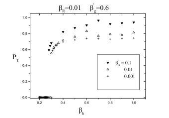
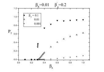
Figure 14: We show the behaviour of $P_{T}$ as the value of $\beta_{h}^{\prime}$ grows. The transition from Strong phase to the $H_{5}$ phase does not seem to change (a), in contrast with the one to from Strong to $H_{4}$ which is washed away (there is a radical change to the value of $P_{T}$ at a critical point of $\beta_{h}$) leading thus to the existence of only a 5D–Higgs phase.

In Figure 14 we depict the behaviour of $P_{T}$ setting $\beta_{R}=0.01$ and for the two cases corresponding to the transitions from the Strong phase to $H_{5}$ and $H_{4}$. The corresponding values for $\beta^{\prime}_{g}$ are 0.6 and 0.2 respectively (see, also, Figure 1). From Figure 14 (a) we can see that as $\beta^{\prime}_{h}$ increases the transition behaviour to $H_{5}$ is fairly the same. On the contrary, Figure 14 (b) shows that the increase in $\beta^{\prime}_{h}$ leads to a big increase in the value of $P_{T}$ which becomes compatible with the value characterizing the $H_{5}$ phase. This provides an indication that at some value, $\beta^{\prime}_{h}\sim 0.1$, the $H_{4}$ phase transforms to $H_{5}$: as $\beta^{\prime}_{h}$ increases $H_{5}$ extends, covering the region occupied before by $H_{4}$.

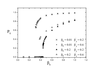
Figure 15: As the value of $\beta_{R}$ increases the $S-H_{4}$ phase transition becomes weaker, as expected, while the $S-H_{5}$ transition remains first order.

Figure 15 provides evidence of the expected weakening of the Strong – $H_{4}$ phase transition as $\beta_{R}$ increases. It reveals that, although for $\beta_{R}=0.01$, $P_{S}$ exhibits the same behaviour for $H_{5}$ and $H_{4}$ phases, for $\beta_{R}=0.2$ the picture changes substantially. The $S-H_{4}$ phase transition provides a sign of a smoother phase transition leading probably to second order. Mone Carlo simulations in this region of parameter space are required to complement this evidence.

4 Conclusions

In this paper, we have shown, using Monte–Carlo methods, that a layered Higgs phase actually exists in the phase diagram of the strongly coupled five–dimensional Abelian Higgs model and that it emerges from the confining bulk phase through a first order phase transition. In fact we find the existence of multi-layers, as each brane passes from the confining phase to the Higgs phase independently of the others.

Using mean field techniques we performed a scan of the phase diagram as the Higgs couplings changed and found evidence that, as the Higgs self-coupling increases, the emergence of the Higgs layers from the confining bulk phase softens and may become second order, leading to new continuum theories. Further work will clarify this issue.

It is worth stressing that the layers of our model are, indeed, 3-branes. In string theory one expects symmetry enhancement when branes coincide and the question arises, whether such an effect could be visible within our field theory context. This effect is the manifestation of new, non-perturbative, degrees of freedom. In our context this would mean introducing magnetic monopoles, that would promote these 3-branes into true D-3-branes. One way of achieving this could be using twisted boundary conditions, along the lines of ref. [9].

This raises the question of what aspects of our study may also be of relevance to Yang-Mills theories [4, 8, 10]. As is well known, these are confining in less than five dimensions, so do not seem to admit four dimensional layered phases. The simplest example would, thus, be an anisotropic $SU(2)$ theory in six dimensions and in this case the layers form an unnatural five–dimensional Coulomb phase . The interesting point would be if the SU(2) Higgs model with extra dimensions could reveal a layered Higgs phase in four dimensions which bears a closer resemblance to the SM. Monte Carlo simulations of such theories directly are, unfortunately, inconclusive with current technology–though the use of massively parallel clusters may offer some hope for the not too distant future. Using suitably reduced models, on the other hand, such as the one studied here, could provide some useful information on their structure.

Acknowledgements

The authors are grateful to G. Koutsoumbas for extensive discussions on the subject during the preparation of the paper and for reading the manuscript. P.D. and K.F. would like to thank A. Kehagias for useful discussions on related topics. Also, P.D. and K.F. acknowledge support from the TMR project “Finite Temperature Phase Transitions in Particle Physics”, EU contract FMRX-CT97-0122.

References

- [1] Y.K. Fu and H.B. Nielsen, Nucl. Phys. B 236, 167 (1984).
- [2] C.P. Korthals-Altes, S. Nicolis and J. Prades, Phys. Lett. B 316 339 (1993) [hep-lat/9306017]; A. Hulsebos, C.P. Korthals-Altes and S. Nicolis, Nucl. Phys. B 450 437 (1995) [hep-th/9406003].
- [3] P. Dimopoulos, K. Farakos, A. Kehagias, G. Koutsoumbas Lattice Evidence for Gauge Field Localization on a Brane [hep-th/0007079].
-
[4]
Guo-Li Wang and Ying-Kai Fu [hep-th/0101146];
Liang-Xin Huang, Ying-Kai Fu and Tian-Lun Chen, J.Phys. G 21 1183 (1995). -
[5]
L. Randall and R. Sundrum, Phys. Rev. Lett. 83
4690 (1999) [hep-th/9906064]; Phys. Rev. Lett. 83 3370
(1999) [hep-ph/9905221];
A. Karch and L. Randall, Int.J.Mod.Phys. A16,780 (2001) [hep-th/0011156]; A. Davidson and P.D. Mannheim, [hep-th/0009064]. -
[6]
W.D. Goldberger and M.B. Wise, Phys. Rev. Lett. 83 4922
(1999) [hep-ph/9907447]; Phys. Rev. D 60 107505 (1999) [hep-ph/9907218];
H. Davoudiasl, J.L. Hewett and T.G. Rizzo, Phys. Lett. B 473 43 (2000) [hep-ph/9911262];
T. Gherghetta and A. Pomarol, Nucl. Phys. B 586 141 (2000) [hep-ph/0003129];
O. DeWolfe, D.Z. Freedman, S.S. Gubser and A. Karch, Phys. Rev. D 62 0406008 (2000) [hep-th/9909134];
A. Kehagias, K. Tamvakis Phys.Lett. B 504:38-46,2001 [hep-th/0010112]; A. Kehagias, Phys. Lett. B 469 123 (1999) [hep-th/9906204]; [hep-th/9911134];
A. Pomarol, Phys. Lett. B 486 153 (2001) [hep-ph/9911294]. - [7] P. Dimopoulos, K. Farakos, G. Koutsoumbas, C.P. Korthals-Altes, S. Nicolis, J. High Energy Phys. 02(005) (2001) [hep-lat/0012028].
- [8] D. Berman and E. Rabinovici, Phys. Lett. 157 B 292 (1985); M. Creutz, Phys. Rev. Lett. 43 553 (1979).
- [9] A. Coste, A. Gonzalez-Arroyo, C. P. Korthals Altes, B. Soderberg and A. Tarancon, Nucl. Phys. B 287 (1987) 569.
- [10] S. Ejiri, J. Kubo and M. Murata, Phys. Rev. D 62 (2000) 105025 [hep-ph/0006217].