UNIGRAZ- UTP-16-05-01 Bound States for Overlap and Fixed Point Actions Close to the Chiral Limit

Abstract

We study the overlap and the fixed point Dirac operators for massive fermions in the two-flavor lattice Schwinger model. The masses of the triplet (pion) and singlet (eta) bound states are determined down to small fermion masses and the mass dependence is compared with various continuum model approximations. Near the chiral limit, at very small fermion masses the fixed point operator has stability problems, which in this study are dominated by finite size effects, however.

PACS: 11.15.Ha, 11.10.Kk
Key words: Lattice field theory, Dirac operator, mass spectrum, Schwinger model

1 Motivation and Introduction

Lattice Dirac operators obeying the Ginsparg-Wilson condition [2] in its simplest form

$$\gamma_{5}\,D+D\,\gamma_{5}=a\,D\,\gamma_{5}\,D\;,$$ (1)

have the advantage to violate chiral symmetry only locally, with quasi automatic ${\cal O}(a)$ improvement. Their eigenvalues lie on a circle in the complex plane; zero eigenvalues correspond to chiral eigenstates and indicate topological (instanton) modes in the gauge field. We known of at least two explicit incarnations of such actions, the so-called overlap action [3] and the perfect action [4]. Both are technically difficult and expensive to determine and to incorporate in a lattice simulation with dynamical fermions.

The Schwinger model (2D fermion-gauge theory with U(1) gauge group) generalized to e.g. 2 flavors provides an attractive model to study such actions. It has similar features like QCD with 2 quark flavors – although due to a quite different underlying dynamics. It has only bosonic bound states, including a massless triplet, and a non-vanishing fermion condensate. The overlap action may be constructed from an arbitrary action, like the Wilson action. It involves a computation of the sign function for hermitian matrices, which has to be repeated for each gauge field and is computationally challenging. A fixed point action (the perfect action determined at the fixed point of the continuum limit) on the other hand has a large number of couplings and is difficult to construct. For the Schwinger model such a fixed point action has been determined in excellent approximation a few years ago [5], at at time, when the spectacular spectral properties of GW-fermion operators were not yet widely discussed. Both, the overlap and the fixed point action then have been studied in the Schwinger model for various aspects, mainly related to the Dirac operator spectrum [6] and to the topological content of the gauge fields.

Introducing mass in the Schwinger model is a subtle problem [7]-[16] and the continuum approximations involve plausible but non-stringent ad-hoc assumptions [8, 16]. Of particular interest is the analog of the PCAC-relation, i.e. the dependence of the triplet bound state mass on the fermion mass parameter. Recent studies for staggered action [17], Wilson action [18] and overlap action [19] have confirmed the exponent $2/3$. Here we try to obtain results closer to the chiral limit for two GW-type actions. The motivation is on one hand further confirmation of the functional dependence and a clearer determination of the correct coefficient.

On the other hand we want to compare the relative merits of these chirally improved actions closer to the chiral limit, which is hardly accessible with e.g. Wilson-type actions. In fact, actions where (near the origin) the eigenvalue spectra scatter have problems at small fermion masses in general. Due to this fluctuation of the small real eigenvalues many configurations will mimic zero modes and necessitate special techniques to deal with them. The hope is to improve this situation with overlap or perfect actions. We discuss our conclusion based on this model study at the end.

2 The massive 2-flavor Schwinger model

We study the euclidean 2d gauge theory with gauge group U(1) and two flavors of fermions with degenerate mass. For vanishing fermion masses, the classical theory has a symmetry group $U(2)_{L}\times U(2)_{R}$ that is broken down by the anomaly to $SU(2)_{L}\times SU(2)_{R}\times U(1)_{V}$. For non-vanishing fermion masses the chiral symmetry is broken at the classical level and a $U(2)_{V}$ symmetry remains.

Let us briefly discuss some known analytical results for the continuum model. The generalized Sine-Gordon model bosonizes the 2-flavor Schwinger model[8]. Its Lagrangian reads

$$\frac{1}{2}\left(\partial\varphi^{(0)}\right)^{2}+\frac{1}{2}\left(\partial\varphi^{(3)}\right)^{2}+\frac{1}{2}\,\frac{2\,g^{2}}{\pi}\left(\varphi^{(0)}\right)^{2}-\frac{m\,c}{\pi}\,\cos\left(\sqrt{2\pi}\,\varphi^{(0)}\right)\cos\left(\sqrt{2\pi}\,\varphi^{(3)}\right)\;.$$ (2)

The constant $c$ is not determined by the bosonization but is related (see e.g. [13, 15]) to the masses $\mu^{(0)}$ and $\mu^{(3)}$ used for normal ordering of the fields $\varphi^{(0)}$ and $\varphi^{(3)}$ by $c=(\mu^{(0)}\mu^{(3)})^{1/2}e^{\gamma}/2$, where $\gamma$ ($=0.577216\ldots$) denotes Euler’s constant. For the case of two flavors two of the currents – which we measure – (compare (14)) are bosonized with the following prescription

$$\overline{\psi}(x)\;\tau^{a}\otimes\gamma_{\mu}\;\psi(x)\;=\;\frac{1}{\sqrt{\pi}}\,\varepsilon_{\mu\nu}\,\partial_{\nu}\;\varphi^{(a)}(x)\quad,\qquad a=0,3\;,$$ (3)

where the generators $\tau^{a}$ of rotations in flavor space are given by the Pauli matrices $\tau^{a}=\sigma_{a},\;a=1,2,3$ and $\tau^{0}\equiv$ 11. For the other two members $j_{\mu}^{(1)},j_{\mu}^{(2)}$ of the iso-triplet no explicit abelian bosonization is known; however due to invariance under flavor rotations, their masses are the same as for the triplet current ($a=3$, which we called pions due to the analog to QCD). For vanishing quark mass $m$ in (2) the two flavor Schwinger model is bosonized by two free fields. One of them, the pion field $\varphi^{(3)}$, is massless ($M_{\pi}=0$) and the eta field $\varphi^{(0)}$ obtains the Schwinger mass $M_{\eta}=g\sqrt{2/\pi}$ (due to the anomaly).

For non-vanishing quark mass, also the bosonized model (2) can no longer be solved in closed form. A semi-classical analysis (see e.g. [15]) should provide a good approximation when all involved masses are large. The squares of the masses are given by the second derivatives of the interaction part $V[\varphi^{(0)},\varphi^{(3)}]$ of (2) at the minimum. After normal ordering the fields $\varphi^{(a)}$ with respect to their own masses (setting $\mu^{(0)}=M_{\eta}$ and $\mu^{(3)}=M_{\pi}$), the semi-classical analysis for the iso-triplet and iso-singlet gives

$$\frac{M_{\pi}}{g}\; = \;e^{2\gamma/3}\;\frac{2^{5/6}}{\pi^{1/6}}\;\left(\frac{m}{g}\right)^{2/3}$$ (4)

$$\frac{M_{\eta}}{g}\; = \;\sqrt{\frac{2}{\pi}\;+\;\left(\frac{M_{\pi}}{g}\right)^{2}}\;.$$ (5)

The first relation plays a role similar to the PCAC relation in QCD (where the pion mass squared is proportional to the quark mass).

In an attempt to go beyond semi-classical analysis one can approximate the generalized Sine-Gordon model (2) by a solvable model. In the limit of large coupling [8] $g$ and small mass $m$ the iso-singlet field $\varphi^{(0)}$ becomes static and the model is reduced to a standard Sine-Gordon model for the triplet field $\varphi^{(3)}$, with the Lagrangian

$$\frac{1}{2}\left(\partial\varphi^{(3)}\right)^{2}\;-\;2C\cos\left(\sqrt{2\pi}\varphi^{(3)}\right)\;.$$ (6)

This reduced bosonized theory has been studied [8, 20] using the WKB approximation [21] and recently again by Smilga [16]. His analysis is now based on the newly derived analytic solution [22] of the standard Sine-Gordon model and he finds

$$\frac{M_{\pi}}{g}\;=\;2^{5/6}\,e^{\gamma/3}\,\left(\frac{\Gamma(\frac{3}{4})}{\Gamma(\frac{1}{4})}\right)^{2/3}\frac{\Gamma(\frac{1}{6})}{\Gamma(\frac{2}{3})}\;\left(\frac{m}{g}\right)^{2/3}\;.$$ (7)

The numerical coefficient of the $(m/g)^{2/3}$ term is 2.008, somewhat smaller than the value 2.1633 in (4). The truncation of the original model (2) to the standard form (6) does not allow for a result for the singlet mass $M_{\eta}$. For this state only the semi-classical formula (5) is available. It his however interesting to use the exact result (7) of the truncated model as an input in (5), and below we compare also this formula to the numerical data.

3 Lattice Dirac Operators

The Schwinger model is a super-renormalizable theory, i.e. the bare coupling does not get renormalized and equals the physical gauge coupling $g$. On the lattice for the standard Wilson plaquette gauge action we use the usual coupling $\beta$ in front of the gauge field action. In the naive continuum limit this is related to the continuum coupling via $\beta=1/g^{2}$ (we set the lattice spacing $a=1$). We define the coupling $g$ which we use for comparison with the analytical results in the continuum (see above) through this relation.

We first generate the massless fermion actions and introduce the fermion mass parameter subsequently.

Overlap Dirac operator

For the overlap action [23] one may start with the Wilson Dirac operator

$$D_{\textrm{\scriptsize Wi}}\,{}(x,y)=(m_{w}+2)\,\delta_{xy}-\frac{1}{2}\sum_{\mu=\hat{1},\hat{2}}\left[(1+\sigma_{\mu})\,U_{xy}\,\delta_{x,y-\mu}+(1-\sigma_{\mu})\,U_{yx}^{\dagger}\,\delta_{x,y+\mu}\right]\;,$$ (8)

(with the Pauli matrices $\sigma_{\mu}$) at some value of $m_{w}\in(-1,0)$ and then construct

$$D_{\textrm{\scriptsize Ov}}\,{}=\frac{1}{2}\left[\textrm{\boldmath{$\mathsf{1}$}}+\gamma_{5}\,\epsilon(\gamma_{5}\,D_{\textrm{\scriptsize Wi}}\,{})\;\right].$$ (9)

Some words about the choice of $m_{w}$: according to [23] it is arbitrary, in the sense that any (strictly negative) value in the interval $(-1,0)$ reproduces the correct continuum theory, but it may be optimized with regard to its scale dependence by looking for example at the behavior of the (projected) spectrum. In many practical determination of the sign function configurations with small eigenvalues of $\gamma_{5}\,D_{\textrm{\scriptsize Wi}}\,{}$ are cumbersome; this situation may be improved by a suitable choice of $m_{w}$. Comparing expectation values of operators like $\langle\bar{\psi}\psi\rangle{}$ for different $m_{w}$ one has to take care of the proper normalization [24]. Comparing with free lattice fermions one finds a (trivial) factor of $\sqrt{2\,m_{w}}$ renormalizing the field operator, i.e. $\langle\bar{\psi}\psi\rangle{}=Z_{\psi}^{-1}\langle\bar{\psi}\psi\rangle{}_{\textrm{\scriptsize Ov}}$ with $Z_{\psi}=|2\,m_{w}|$ in our convention. We choose $m_{w}=-1$.

The operative definition of the generalized sign function $\epsilon(\gamma_{5}\,D_{\textrm{\scriptsize Wi}}\,{})$ entering the above equation is through its eigenvalues,

$$\epsilon(\gamma_{5}\,D_{\textrm{\scriptsize Wi}}\,{})=U\,\textrm{Sign}(\Lambda)\,U^{\dagger}\quad\textrm{with}\;\gamma_{5}\,D_{\textrm{\scriptsize Wi}}\,{}=U\,\Lambda\,U^{\dagger}\;.$$ (10)

Here $\textrm{Sign}(\Lambda)$ denotes the diagonal matrix containing the signs of the eigenvalues obtained through the unitary transformation $U$ of the hermitian matrix $\gamma_{5}\,D_{\textrm{\scriptsize Wi}}\,{}$. There are various ways to numerically find $D_{\textrm{\scriptsize Ov}}\,$without passing through the diagonalization problem (which is prohibitively expensive for $D=4$) [25, 26, 27] (for $D=2$ see also [28] and recently, in the Schwinger model [29, 19]). In our simple context computer time is no real obstacle and therefore we use the direct definition (10), explicitly performing the diagonalization. For comparison we also applied an iterative technique implementing Newton’s method [25, 28]. For many gauge configurations the resulting operators agreed to the requested accuracy (8 digits). For larger $\beta\geq 4$ however, the number of configurations with convergence problems for the iterative method due to small eigenvalues increased. The results presented here are all based on the exact diagonalization.

Fixed point Dirac operator

In Ref.[5] the fixed point Dirac operator was parameterized as

$$D_{\textrm{\scriptsize Fp}}\,{}(x,y)=\frac{1}{2}\,\sum_{i=0}^{3}\sum_{x\,,f}\,\rho_{i}(f)\,\sigma_{i}\,U(x,f)\;,\quad\textrm{with}\;y\equiv x+\delta f\;.$$ (11)

Here $f$ denotes a closed loop through $x$ or a path from the lattice site $x$ to $y=x+\delta f$ (distance vector $\delta f$) and $U(x,f)$ is the parallel transporter along this path. The $\sigma_{i}$-matrices denote the Pauli matrices for $i=1,2,3$ and the unit matrix for $i=0$. Note the factor $1/2$ in (11) in order to obtain the same normalization as the overlap Dirac operator. The action obeys the usual symmetries as discussed in [5]; altogether it has 429 terms per site. The action was originally determined at large $\beta$ for gauge fields distributed according to the non-compact formulation with the Gaussian measure. Excellent scaling properties, rotational invariance and continuum-like dispersion relations were observed at various smaller values of the gauge coupling $\beta$.

In Ref.[6] this action was studied both, for compact and the original non-compact gauge field distributions. In the compact case the action is not expected to exactly reproduce the fixed point of the corresponding BST, but nevertheless it is still a solution of the GWC (1); violations are instead introduced by the parameterization procedure, which cuts off the less local couplings. It was demonstrated, that the eigenvalue spectrum is close to circular shape, improving in this respect towards larger $\beta$ (see [30] for a more detailed discussion).

Here we study the action only for the compact gauge field distributions in order to allow for a direct comparison with the overlap Dirac operator.

The massive case

The massive overlap Dirac operator may be related to the massless one by [31]

$$D_{\textrm{\scriptsize Ov}}\,{}(\mu)=(1-\mu)\left[D_{\textrm{\scriptsize Ov}}\,{}(0)+\frac{\mu}{1-\mu}\right]\;,$$ (12)

where the mass parameter $-1<\mu<1$ is related to the fermion mass by

$$m=\mu\,Z_{m}^{-1}(1+\mathcal{O}(a^{2})),$$ (13)

with $Z_{\psi}Z_{m}=1$, where $Z_{m}$ and $Z_{\psi}$ are the mass and the wavefunction renormalization constants, respectively. Since with our choice of parameterization the massless fixed point Dirac operator (11) has the same overall renormalization as the massless overlap Dirac operator (9) we also use (12) to generate the massive fixed point Dirac operator.

4 Simulation Details

Uncorrelated gauge configurations for lattice size $16^{2}$ and $24^{2}$ have been generated in the quenched setup. However, we are including the fermionic determinant in the observables: all the results presented here are obtained with the correct determinant (squared, for two flavors) weight. From earlier experience [5, 6] we learned that this is justifiable for this model and the presented statistics. We perform our investigation on two sets of 5000-10000 configurations at $\beta=4$ and 6. These are the same gauge configurations as used in Ref.[18] for the determination of bound state masses for the Wilson Dirac operator and thus we may compare the relative efficiency in the results.

The configurations have been well separated by three times the autocorrelation length for the so-called “geometric definition” of the topological charge. For each configuration we construct $D_{\textrm{\scriptsize Ov}}\,$and $D_{\textrm{\scriptsize Fp}}\,$as discussed. For each lattice Dirac matrix we then compute the inverse (the quark propagator) and the determinant.

The masses for the pions and the eta-particle were determined from the decay of two point functions of the following vector currents

$$J_{x}^{a\mu} = \overline{\psi}_{x}\;\tau^{a}\otimes\gamma_{\mu}\;\psi_{x}\;\;\;\;\;\mbox{for the $\pi$'s}\;,$$

$$J_{x}^{0\mu} = \overline{\psi}_{x}\;\mbox{11}\otimes\gamma_{\mu}\;\psi_{x}\;\;\;\;\;\;\;\mbox{for the}\;\eta\;.$$ (14)

We emphasize that 2-point functions of scalars or pseudo-scalars are not particularly well suited for the determination of the meson masses. These operators are bosonized (compare the discussion above) by cosines and sines of the fundamental fields [9, 13] and their 2-point functions strongly mix contributions from both the triplet and singlet states. For the two point functions of the momentum-zero projected vector currents one has to take care about the proper choice of $\mu$. As could be verified by gauge field integration there are no contributions to the propagation of $J_{x}^{a2}(p=0)$ in the direction $\mu=2$.

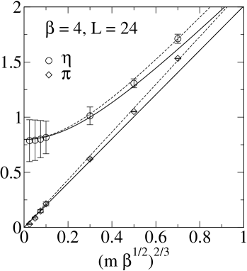
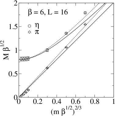
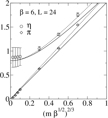
Figure 1: Results for overlap Dirac operator $\beta=4$, 6, $L=16$, 24. Symbols: Monte Carlo data. Full line: Smilga’s formula (7). Dashed line: the semi-classical approximation (4) and (5).

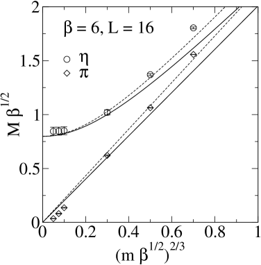
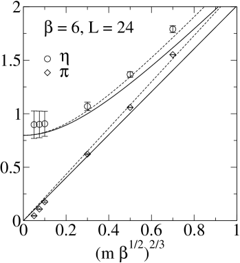
Figure 2: Results for the fixed point Dirac operator at $\beta=6$, $L=16$, 24. Symbols: Monte Carlo data. Full line: Smilga’s formula (7). Dashed line: the semi-classical approximation (4) and (5).

5 Results

Let us now discuss our numerical results for the mass spectrum. We present the data for the overlap Dirac operator for $\beta=4$ and 6 and $L=16$ and 24 in Fig. 1. The results for the fixed point operator at $\beta=6$ and $L=16,24$ are shown in Fig. 2. In each plot we combine the values of the singlet mass and the triplet mass and compare the numerical results to Smilga’s formula (7) (full lines) and the semi-classical results (4) and (5)(dotted lines).

We observe that the data are well described by the semi-classical result (4) (dotted line). In particular at quark masses above $(m\sqrt{\beta})^{2/3}\geq 0.3$ the semi-classical approximation is fulfilled best. In this region our results for the triplet mass coincide with the results of [19]. For small quark masses we observe a strong and seemingly systematic deviation especially for small lattice size. We attribute this to finite size effects. In particular, the boson propagator does not really become asymptotic at such large correlation lengths.

For the fixed point operator we only get reasonably results for small $m$ at large gauge couplings $\beta\geq 4$, when the spectrum is close to circular. For smaller $\beta$ the scattering of the small eigenvalues is too large and of the order of the bare fermion mass parameter, causing disturbing fluctuations. The dispersion $\sigma$ of the eigenvalues around the circle (which decreases with larger $\beta$[30]) leads to accidental poles in the propagators even at non-vanishing quark mass.

For the eta mass $M_{\eta}$ we find that the data approach the correct $m=0$ value as the quark mass vanishes. The semi-classical formula (5) provides a reasonable description of the data. For small $m$ the quantum fluctuations become larger and thus the numerical data deviate from the semi-classical curve. The cases with comparatively large error bars always indicate lack of sufficient statistics for the propagator. The behavior at small $m$ can be fitted by a power law as has been done in Ref.[17] for the results from the model with staggered fermions.

Comparing the results with those obtained in Ref.[18] for the Wilson Dirac operator we find generally smoother behavior, in particular at smaller fermion mass parameters. This was to be expected due to the improved chirality properties. On the other hand, for a full exploitation of this feature larger lattices with better finite size control are needed.

6 Conclusion

We find that our results for the singlet mass and the triplet mass are well described by the semi-classical formulas (4), (5). For the triplet mass $M_{\pi}$ we observe a clear deviation from the semi-classical curve at small quark masses which we attribute to finite volume effects. For the $\eta$-mass the data are in good agreement with the semi-classical approximantion with quantum fluctuations becoming less important as the quarks are made heavier.

As for the studied model, although the results for $\eta$ and $\pi$ are in good agreement with the the analytic expectations the values of the pion mass below $M_{\pi}\sqrt{\beta}<0.3$ are clearly plagued by the limited lattice size. However, our emphasis was on the study of the effects due to the chiral properties of the Dirac operators. For better results for the $\pi$-mass at very small masses much larger lattice and higher statistics appear to be necessary to allow a control of the finite size effects.

For small fermion masses it seems to be important, that the eigenvalues of the Dirac operator do not scatter too much away from the optimal unit circle. With this regard the overlap action does the better job. Even the qualitatively quite good fixed point action exhibits a weakness for small $\beta$ due to this effect. Spurious singularities or almost-singularities in the propagator necessitate very large samples in order to obtain reliable mean expectation values and thus propagators. The width of the distribution of eigenvalues around zero therefore essentially limits the practically applicable values of the bare fermion mass parameter.

Acknowledgment: We want to thank C. Gattringer and I. Hip for many useful discussions.

References

- [1]
- [2] P. H. Ginsparg and K. G. Wilson, Phys. Rev. D 25 (1982) 2649
- [3] R. Narayanan and H. Neuberger, Phys. Lett. B302 (1993) 62; Phys. Rev. Lett. 71 (1993) 3251; Nucl. Phys. B412 (1994) 574; ibid. B443 (1995) 305.
- [4] P. Hasenfratz and F. Niedermayer, Nucl. Phys. B414 (1994) 785; P. Hasenfratz, Nucl. Phys. B (Proc. Suppl.) 63 (1998) 53; P. Hasenfratz et al., Nucl. Phys. B (Proc.Suppl.) 94 (2001) 627.
- [5] C. B. Lang and T. K. Pany, Nucl. Phys. B513 (1998) 645.
- [6] F. Farchioni, C. B. Lang and M. Wohlgenannt, Phys. Lett. B433 (1998) 377.
- [7] S. Coleman, R. Jackiw and L. Susskind, Ann. Phys. 93 (1975) 267.
- [8] S. Coleman, Ann. Phys. 101 (1976) 239.
- [9] L. V. Belvedere et al., Nucl. Phys. B153 (1979) 112.
- [10] H. Joos, Helv. Phys. Acta 63 (1990) 670; S. I. Azakov and H. Joos, Helv. Phys. Acta 67 (1994) 723; I. Sachs and A. Wipf, Helv. Phys. Acta 95 (1992) 652.
- [11] M. P. Fry, Phys. Rev. D47 (1993) 2629; Phys. Rev. D51 (1995) 810;
- [12] C. Adam, Ann. Phys. 259 (1997) 1.
- [13] C. Gattringer and E. Seiler, Ann. Phys. 233 (1994) 97.
- [14] J. E. Hetrick, Y. Hosotani and S. Iso, Phys. Lett. B 350 (1995) 92.
- [15] C. Gattringer, Ann. Phys. 250 (1996) 389 and QED2 and U(1)-problem, Thesis, University of Graz 1995 (E-Print hep-th/9503137).
- [16] A. V. Smilga, Phys. Rev. D55 (1997) 443.
- [17] C. Gutsfeld et al., Nucl. Phys. Proc. Suppl. 63 (1998) 266; Nucl. Phys. B560 (1999) 431.
- [18] C. Gattringer, I. Hip and C. B. Lang, Phys. Lett. B466 (1999) 287.
- [19] L. Giusti, C. Hoelbling and C. Rebbi, Nucl. Phys. Proc. Suppl. 94 (2001) 741; E-Print hep-lat/0101015.
- [20] M. Grady, Phys. Rev. D35 (1987) 1961; Nucl. Phys. B365 (1991) 699.
- [21] R. F. Dashen, B. Hasslacher and A. Neveu, Phys. Rev. D11 (1975) 3424.
- [22] A. B. Zamolodchikov, Int. J. Mod. Phys. A10 (1995) 1125.
- [23] H. Neuberger, Phys. Lett. B417 (1998) 141; ibid. B353 (1998) 427.
- [24] Y. Kikukawa, R. Narayanan and H. Neuberger, Phys. Rev. D57 (1998) 1233.
- [25] H. Neuberger, Phys. Rev. Lett. 81 (1998) 4060.
- [26] R. G. Edwards, U. M. Heller and R. Narayanan, Nucl. Phys. B540 (1999) 457.
- [27] P. Hernández, K. Jansen and M. Lüscher, Nucl. Phys. B552 (1999) 393; P. Hernández, K. Jansen and L. Lellouch, E-print hep-lat/0001008
- [28] T.-W. Chiu, Phys. Rev. D58 (1998) 074511.
- [29] L. Giusti, C. Hoelbling and C. Rebbi, Nucl. Phys. Proc. Suppl. 83 (2000) 896.
- [30] F. Farchioni et al., Nucl. Phys. Proc. Suppl. 73 (1999) 939; Nucl. Phys. B549 (1999) 364.
- [31] R. G. Edwards, U. M. Heller and R. Narayanan, Phys. Rev. D59 (1999) 094510.