Effective Lagrangian for strongly coupled domain wall fermions

Abstract

We derive the effective Lagrangian for mesons in lattice gauge theory with domain-wall fermions in the strong-coupling and large-$N_{c}$ limits. We use the formalism of supergroups to deal with the Pauli-Villars fields, needed to regulate the contributions of the heavy fermions. We consider the spectrum of pseudo-Goldstone bosons and show that domain wall fermions are doubled and massive in this regime. Since we take the extent and lattice spacing of the fifth dimension to infinity and zero respectively, our conclusions apply also to overlap fermions.

I Introduction

From its inception, lattice gauge theory was hampered by the absence of an adequate fermion formulation. It was thought for many years that there is no discretization scheme that displays explicit chiral symmetry without either sacrificing locality or introducing non-physical doublers in the fermion spectrum. This state of affairs was summarized in the famous no-go theorem of Nielsen and Ninomiya [1]. Recent years have seen major progress in the construction of lattice regularizations of fermions with good chiral properties [2]. Domain wall [3] and overlap [4] formulations preserve chiral symmetry exactly, allowing the construction of vector gauge theories on the lattice. An idea common to these schemes is that of employing a large number of fermion flavors, one of which survives in the continuum limit as a massless fermion supporting exact chiral symmetry.

In the domain wall formulation, the expanded flavor space may be seen as an extra dimension with a defect in a background field. One chirality of the Dirac spinor is exponentially localized along the defect. If the extra dimension is periodic and of finite extent $L_{5}$, the other chirality will be localized along an unavoidable second defect, while all the other Dirac fermions, $L_{5}-1$ in number, stay heavy. This is also the scheme in Shamir’s surface-fermion variant [5, 6], which we study in this paper; here the chiral modes are localized on the surfaces of a five-dimensional slab. In either case, the limit $L_{5}\rightarrow\infty$ requires that the contribution of the heavy flavors be subtracted [4, 6, 7, 8] by introducing $L_{5}$ flavors of pseudofermion fields, often called Pauli-Villars (PV) fields. These are bosons that have the same index structure as the fermions.

Domain wall fermions are equivalent to overlap fermions [4] in the limit that the size and lattice spacing of the fifth dimension are taken to infinity and zero, respectively [7, 9]. The bulk degrees of freedom remain massive. They decouple as the four-dimensional lattice is removed, leaving a four-dimensional Dirac operator describing the chiral surface modes.

In this paper we study domain wall fermions in the limit of strong gauge coupling. We adapt the classic method of Kawamoto and Smit [10] to derive an effective action for mesonic degrees of freedom. A novel ingredient of the domain wall formalism is the PV bosons. We combine the fermions and pseudofermions into a supervector, and similarly group the effective degrees of freedom into a supermatrix. Then the formalism of supergroups allows us easily to extend the treatment of the fermions to an analysis of the complete theory. The effective action contains all the meson-like states that can be constructed from pairs of fermions, from pairs of bosons, and from boson-fermion pairs.

The interesting question is, does this theory really behave as one would expect of a theory of exactly chiral quarks? To address this, we take the number of colors $N_{c}$ to infinity and look for saddle points of the effective action. Following Kawamoto and Smit, we begin by setting the Wilson parameter $r$ to zero and classifying the symmetries of the theory; we display explicitly the Goldstone bosons that are the fluctuations around the saddle point. The spectrum of Goldstone bosons is characteristic of a theory with complete fermion doubling, which is not surprising since it is the term proportional to $r$ in the fermion action that breaks naive doubling in the first place. When we proceed, however, to perturb the saddle point with the $r$ terms, we find that the doubling persists and that the only effect of the perturbation is identical to that of adding a mass term (à la Shamir [5, 6]) to the domain wall action. We conclude that in the strong coupling limit, domain wall fermions are doubled and massive, with all that that implies for the mesonic spectrum.

We thus confirm the conclusion reached by two of us [16] through study of the Hamiltonian of domain wall fermions at strong coupling. Unfortunately, our analysis here is more involved and perhaps less conclusive. Study of the Hamiltonian via Rayleigh-Schrödinger perturbation theory is straightforward and leads unambiguously to an effective Hamiltonian for mesonic degrees of freedom. The symmetries of this effective theory are readily apparent. In the Euclidean formulation some additional approximation is necessary, such as a hopping parameter expansion, mean field theory, or the large-$N_{c}$ limit. Even at large $N_{c}$, one might argue that there exists another saddle point with different symmetry properties. Nonetheless, the Euclidean study complements the Hamiltonian results in that it does not require a time-continuum limit and thus does not introduce a new question regarding the order of limits.

In Sec. II we derive the strong-coupling effective action. For pedagogic reasons, we begin by ignoring the PV bosons. Following Kawamoto and Smit [10], we integrate out the gauge field in this limit and rewrite the resulting path integral in terms of a bosonic matrix field. That this path integral generates the same Green functions as the original Grassmann integral is due to an equality between generating functions that was proven in [10] (following [19]). This path integral contains the effective action. While its derivation does not depend on a large-$N_{c}$ limit, we give its explicit form for this case only. In the last part of Sec. II we repeat the derivation with the bosons included. This requires a generalization to supermatrices of the identity relating generating functions, which we prove in Appendix B.

Since the chiral symmetry of the domain wall action arises dynamically, it is difficult to analyze the symmetry of the effective action directly. The symmetry analysis cannot be divorced from the dynamics. Section III is devoted to deriving the symmetry breaking pattern of the theory and the spectrum of Goldstone bosons. We can only make analytic progress in the $N_{c}\to\infty$ limit. Here the task at hand is to find saddle points of the effective action. Again we start with an analysis of the theory without the PV bosons. We begin by setting $r$ to zero which makes finding a saddle point straightforward. In this limit the symmetry of the effective action is apparent; upon introducing an ansatz for the saddle point we display the pattern of spontaneous symmetry breaking and the concomitant Goldstone bosons. Then we turn on the Wilson term in the action and we compute its effect on the saddle point. It turns out that the degeneracy of the $r=0$ saddle point is broken by the $r$ term, but only in the way that a mass term breaks it, that is, by breaking chiral symmetry while leaving the doubling. We show explicitly that inclusion of the Shamir mass term does the same.

The extension of the calculation to include the PV bosons is straightforward. The saddle point in the enlarged field space is the obvious extension of the saddle point found above. Perturbing the saddle point with the Wilson term of the bosonic fields gives a mass matrix for the pseudo-Goldstone bosons that is identical in form to that due to the massive fermions.

We conclude with some discussion and comparison to other work.

II The Effective Action at Strong Coupling and Large $N_{c}$

A Without Pauli-Villars bosons

We define domain wall fermions on a five-dimensional hypercubic lattice. The fifth dimension has finite extent $L_{5}$; for generality we assign a lattice spacing $a$ to the four dimensions of Euclidean space-time and a separate lattice spacing $a_{5}$ to the fifth dimension. We shall denote by $x=(x_{1},x_{2},x_{3},x_{4})$ a coordinate vector in the four dimensional space, with Greek indices $\mu,\nu,\ldots$; the fifth coordinate is $s$. The fermion field $\psi^{a\alpha}_{xs}$ is a Grassmann field carrying color index $a=1,\ldots,N_{c}$ and Dirac-flavor index $\alpha=1,\ldots,4N_{f}$. The gauge field $U_{x\mu}$ is an $SU(N_{c})$ matrix field that resides on the four-dimensional links only and is independent of $s$.

The action is a sum of pure-gauge and Dirac actions,

$$S(U,\bar{\psi},\psi)=S_{U}(U)+S_{F}(\bar{\psi},\psi,U).$$ (1)

The gauge action is as usual a sum over plaquettes,

$$S_{U}=\frac{2N_{c}}{g^{2}}\sum_{P}\left(1-\frac{1}{N_{c}}\text{Re}\,\text{Tr}\,U_{P}\right).$$ (2)

We write the fermion action as

$$S_{F}=S_{4}+S_{5}+S_{m},$$ (3)

with

$$S_{4} = \sum_{xs\mu}\left[\bar{\psi}^{a\alpha}_{xs}\left(\frac{r+\gamma_{\mu}}{2}\right)_{\alpha\beta}U_{x\mu}^{ab}\psi^{b\beta}_{x+\hat{\mu},s}+\bar{\psi}^{a\alpha}_{x+\hat{\mu},s}\left(\frac{r-\gamma_{\mu}}{2}\right)_{\alpha\beta}U_{x\mu}^{{\dagger}ab}\psi^{b\beta}_{xs}\right],$$ (4)

$$S_{5} = \rho\sum_{x}\sum_{s=1}^{L_{5}-1}\left[\bar{\psi}^{a\alpha}_{xs}\left(\frac{1+\gamma_{5}}{2}\right)_{\alpha\beta}\psi^{a\beta}_{x,s+1}+\bar{\psi}^{a\alpha}_{x,s+1}\left(\frac{1-\gamma_{5}}{2}\right)_{\alpha\beta}\psi^{a\beta}_{xs}\right],$$ (5)

$$S_{m} = (m-4-\rho)\sum_{xs}\bar{\psi}^{a\alpha}_{xs}\psi^{a\alpha}_{xs},$$ (6)

and $\rho=a/a_{5}$. Only $S_{4}$ contains the gauge field.

In the strong-coupling limit we drop $S_{U}$. The effective action will then be written in terms of the meson field,

$${\cal M}^{\alpha\beta}_{ss^{\prime}}(x)=\frac{1}{N_{c}}\sum_{a=1}^{N_{c}}\psi_{xs}^{a\alpha}\bar{\psi}_{xs^{\prime}}^{a\beta}\;.$$ (7)

This is a color singlet, local in $x$ but nonlocal in $s$, and hence we write it as a $(4N_{f}L_{5})\times(4N_{f}L_{5})$ matrix. (This is in line with the view that $s$ represents an internal flavor index. Eventually we will isolate the projection of ${\cal M}$ onto the subspace spanned by the chiral surface modes.)

In the strong-coupling limit the partition function is given by

$$Z=\int{\cal D}\bar{\psi}\,{\cal D}\psi\,{\cal D}U\,\exp S_{F}(\bar{\psi},\psi,U)$$ (8)

The integral over the gauge field can be performed immediately by noting that it is simply a product of decoupled link integrals,

$$e^{S_{1}(\bar{\psi},\psi)} \equiv \int{\cal D}U\,\exp S_{4}(\bar{\psi},\psi,U)$$ (9)

$$= \prod_{x\mu}\int dU\,\exp\text{Tr}\,[\bar{A}_{\mu}(x)U+U^{\dagger}A_{\mu}(x)],$$ (10)

where we have defined

$$\bar{A}^{ba}_{\mu}(x) = \sum_{s}\bar{\psi}^{a\alpha}_{xs}\left(\frac{r+\gamma_{\mu}}{2}\right)_{\alpha\beta}\psi^{b\beta}_{x+\hat{\mu},s},$$ (11)

$$A^{ba}_{\mu}(x) = \sum_{s}\bar{\psi}^{a\alpha}_{x+\hat{\mu},s}\left(\frac{r-\gamma_{\mu}}{2}\right)_{\alpha\beta}\psi^{b\beta}_{xs}.$$ (12)

The integral in Eq. (10) can be carried out explicitly for any value of $N_{c}$ [20], and the result expressed in terms of ${\cal M}(x)$. We are interested in the limit $N_{c}\to\infty$ [21, 22]. Defining

$$\lambda_{\mu}(x)=-4{\cal M}(x)\frac{r+\gamma_{\mu}}{2}{\cal M}(x+\hat{\mu})\frac{r-\gamma_{\mu}}{2},$$ (13)

the result is

$$S_{1}({\cal M})=N_{c}\sum_{x\mu}\text{tr}\,F(\lambda_{\mu}(x)),$$ (14)

where

$$F(\lambda)=1-\sqrt{1-\lambda}+\log\left[\frac{1}{2}\left(1+\sqrt{1-\lambda}\ \right)\right].$$ (15)

The trace (“tr”) in Eq. (14) denotes a trace over Dirac-flavor and $s$ indices, not to be confused with the color trace (“Tr”) appearing in Eq. (2). We plot $F(\lambda)$ in Fig. 1, and note that one may use a straight line $F(\lambda)\simeq\lambda/4$ as a first approximation.

The remainder of $S_{F}$ couples fields along the fifth axis for fixed $x$. We can rewrite this in terms of $\cal M$ as well, viz.,

$$S^{\perp}\equiv S_{5}+S_{M}=-N_{c}\sum_{x}\text{tr}\,D^{\perp}{\cal M}(x),$$ (16)

where we denote by $D^{\perp}$ the fifth-dimension Wilson-Dirac operator,

$$D^{\perp}_{ss^{\prime}}=\rho\left[\left(\frac{1+\gamma_{5}}{2}\right)\delta_{s,s^{\prime}-1}+\left(\frac{1-\gamma_{5}}{2}\right)\delta_{s,s^{\prime}+1}\right]+(m-4-\rho)\delta_{s,s^{\prime}},$$ (17)

with implicit limits on $s$ and $s^{\prime}$ as indicated in Eq. (5). The complete partition function is then

$$Z(J)=\int{\cal D}\bar{\psi}\,{\cal D}\psi\,\exp\left[S_{1}({\cal M})+S^{\perp}({\cal M})+S_{J}(J,{\cal M})\right],$$ (18)

where we have added an external current coupled to mesonic bilinears according to

$$S_{J}=\sum_{xss^{\prime}}\bar{\psi}^{a\alpha}_{xs}J_{ss^{\prime}}^{\alpha\beta}(x)\psi_{xs^{\prime}}^{a\beta}=-N_{c}\sum_{x}\text{tr}\,J(x){\cal M}(x)$$ (19)

so that functional differentiation with respect to $J$ generates Green functions of the fermion bilinear field ${\cal M}(x)$.

As shown in [10], the same Green functions are generated by the purely bosonic partition function

$$Z(J)=\int{\cal D}M(x)\,\exp\left[-N_{c}\sum_{x}\text{tr}\,\log M(x)\right]\exp\left[S_{1}(M)+S^{\perp}(M)+S_{J}(J,M)\right].$$ (20)

Here $M(x)\in U(4N_{f}L_{5})$ is a bosonic, unitary matrix field and ${\cal D}M(x)$ indicates the invariant Haar measure at each 4d site $x$. (We derive this result in Appendix B, and generalize it to include Pauli-Villars fields.) Collecting everything, we have

$$Z(J)=\int{\cal D}M(x)\,e^{S_{\text{eff}}(M)},$$ (21)

with

$$S_{\text{eff}}(M) = N_{c}\left[\sum_{x,\mu}\text{tr}\,F\Bigl{(}-M(x)(r+\gamma_{\mu})M(x+\hat{\mu})(r-\gamma_{\mu})\Bigr{)}-\sum_{x}\text{tr}\,D^{\perp}M(x)\right.$$ (23)

$$\qquad\left.-\sum_{x}\text{tr}\,\log M(x)-\sum_{x}\text{tr}\,J(x)M(x)\right].$$

We set $J=0$ henceforth.

The fifth-dimension Wilson-Dirac operator $D^{\perp}$ is not hermitian. It will be convenient to work with the hermitian operator $h\equiv\gamma_{4}D^{\perp}$, so we substitute $M\to M\gamma_{4}$, giving

$$S_{\text{eff}}(M) = N_{c}\left[\sum_{x,\mu}\text{tr}\,F\Bigl{(}-M(x)\gamma_{4}(r+\gamma_{\mu})M(x+\hat{\mu})\gamma_{4}(r-\gamma_{\mu})\Bigr{)}-\sum_{x}\text{tr}\,hM(x)\right.$$ (25)

$$\qquad\left.-\sum_{x}\text{tr}\,\log M(x)\right].$$

The measure and $\text{tr}\,\log M$ are unchanged since $\gamma_{4}$ is a special unitary matrix. $h$ is precisely the single-site Hamiltonian studied (in the $a_{5}\to 0$ limit) in [16]. We review its spectrum and eigenfunctions in Appendix A.

B Addition of Pauli-Villars bosons

We have so far neglected the Pauli-Villars fields. Introduction of supermatrix notation will enable us easily to extend our calculation to include their effects in the effective action.

Following Vranas [8], we introduce scalar fields $\phi_{xs}^{a\alpha}$ and their conjugates, with the same indices as the fermions. Their action $S_{PV}(\bar{\phi},\phi)$ is identical in form to the fermion action $S_{F}$ [see Eqs. (3)–(6)]. The only difference is the imposition of antiperiodic boundary conditions instead of the free surfaces at $s=1$ and $s=L_{5}$, which we write as a modification of $S_{5}$,

$$S_{5}\to\rho\sum_{x}\sum_{s=1}^{L_{5}}\left[\bar{\phi}^{a\alpha}_{xs}\left(\frac{1+\gamma_{5}}{2}\right)_{\alpha\beta}\phi^{a\beta}_{x,s+1}+\bar{\phi}^{a\alpha}_{x,s+1}\left(\frac{1-\gamma_{5}}{2}\right)_{\alpha\beta}\phi^{a\beta}_{xs}\right],$$ (26)

where

$$\phi_{x,L_{5}+1}^{a\alpha}=-\phi_{x1}^{a\alpha}.$$ (27)

We group $\psi$ and $\phi$ into a superfield,

$${\Psi_{xs}^{a\alpha}=\left(\begin{array}[]{c}\psi_{xs}^{a\alpha}\\ \phi_{xs}^{a\alpha}\end{array}\right).}$$ (28)

The generalized meson field is a supermatrix containing Grassmann elements as well as ordinary numbers,

$${\cal M}^{\alpha\beta}_{ss^{\prime}}(x)=\frac{1}{N_{c}}\sum_{a=1}^{N_{c}}\Psi_{xs}^{a\alpha}\bar{\Psi}_{xs^{\prime}}^{a\beta}=\frac{1}{N_{c}}\sum_{a=1}^{N_{c}}\left({\begin{array}[]{cc}\psi_{xs}^{a\alpha}\bar{\psi}_{xs^{\prime}}^{a\beta}&\psi_{xs}^{a\alpha}\bar{\phi}_{xs^{\prime}}^{a\beta}\\ \phi_{xs}^{a\alpha}\bar{\psi}_{xs^{\prime}}^{a\beta}&\phi_{xs}^{a\alpha}\bar{\phi}_{xs^{\prime}}^{a\beta}\end{array}}\right).$$ (29)

It is a $(4N_{f}2L_{5})\times(4N_{f}2L_{5})$ matrix that contains the old meson matrix (7) in the upper left-hand corner.

In the strong coupling limit the partition function is now

$$Z=\int{\cal D}\bar{\psi}\,{\cal D}\psi\,{\cal D}\bar{\phi}\,{\cal D}\phi\,{\cal D}U\,\exp\left[S_{F}(\bar{\psi},\psi,U)+S_{PV}(\bar{\phi},\phi,U)\right].$$ (30)

We integrate out the gauge fields as we did in Eq. (10),

$$e^{S_{1}(\bar{\psi},\psi,\bar{\phi},\phi)} \equiv \int{\cal D}U\,\exp[S_{4}(\bar{\psi},\psi,U)+S_{4}(\bar{\phi},\phi,U)]$$ (31)

$$= \prod_{x\mu}\int dU\,\exp\text{Tr}\,[\bar{A}_{\mu}(x)U+U^{\dagger}A_{\mu}(x)],$$ (32)

where we have defined, in analogy with Eqs. (11) and (12),

$$\bar{A}^{ba}_{\mu}(x) = \sum_{s}\bar{\Psi}^{a\alpha}_{xs}\left(\frac{r+\gamma_{\mu}}{2}\right)_{\alpha\beta}\Psi^{b\beta}_{x+\hat{\mu},s},$$ (33)

$$A^{ba}_{\mu}(x) = \sum_{s}\bar{\Psi}^{a\alpha}_{x+\hat{\mu},s}\left(\frac{r-\gamma_{\mu}}{2}\right)_{\alpha\beta}\Psi^{b\beta}_{xs}.$$ (34)

Performing the integral (32) in the limit $N_{c}\to\infty$ we obtain [cf. Eq. (14)]

$$S_{1}({\cal M})=N_{c}\sum_{x\mu}\text{Str}\,F(\lambda_{\mu}(x)),$$ (35)

where Str denotes the supertrace (see Appendix B). $F$ and $\lambda$ are the same as before, with $\lambda$ defined in terms of the new supermatrix field ${\cal M}$. The equivalent of Eq. (16) is

$$S^{\perp}=-N_{c}\sum_{x}\text{Str}\,D^{\perp}{\cal M}(x),$$ (36)

where the new $D^{\perp}$ is defined by

$$D^{\perp}=\left(\begin{array}[]{cc}D^{\perp}_{F}&0\\ 0&D^{\perp}_{PV}\\ \end{array}\right).$$ (37)

Here $D^{\perp}_{F}$ is the fermionic fifth-dimension Wilson-Dirac operator given in Eq. (17); the Wilson-Dirac operator $D^{\perp}_{PV}$ for the bosons is derived from Eq. (26) and differs from $D^{\perp}_{F}$ only on the boundaries. Thus we arrive again at Eq. (18),

$$Z=\int{\cal D}\bar{\Psi}\,{\cal D}\Psi\,\exp\left[S_{1}({\cal M})+S^{\perp}({\cal M})\right],$$ (38)

mutatis mutandis.

We show in Appendix B that the integral over the superfield $\Psi$ can be replaced by an integral over a supermatrix field $M$,

$$Z=\int{\cal D}M(x)\,\exp\left[-N_{c}\sum_{x}\text{Str}\,\log M(x)\right]\exp\left[S_{1}(M)+S^{\perp}(M)\right].$$ (39)

In this equation $M(x)$ is an element of the supergroup $U(4N_{f}L_{5}|4N_{f}L_{5})$ and ${\cal D}M(x)$ is the corresponding invariant Haar measure at each 4d site $x$. Since $D^{\perp}$ is not hermitian, we again substitute $M\rightarrow M\gamma_{4}$ and define the hermitian operator $h=\gamma_{4}D^{\perp}$. The result is

$$S_{\text{eff}}(M) = N_{c}\left[\sum_{x,\mu}\text{Str}\,F\Bigl{(}-M(x)\gamma_{4}(r+\gamma_{\mu})M(x+\hat{\mu})\gamma_{4}(r-\gamma_{\mu})\Bigr{)}-\sum_{x}\text{Str}\,hM(x)\right.$$ (41)

$$\qquad\left.-\sum_{x}\text{Str}\,\log M(x)\right].$$

This is the effective action for all the meson-like degrees of freedom.

III Chiral symmetry breaking pattern and Goldstone bosons

The large-$N_{c}$ limit allows us to evaluate the partition function by finding saddle points of the effective actions (25) and (41). We shall begin by setting $r=0$, whereupon Wilson fermions reduce to naive fermions, and then we will see how things change as the Wilson term is restored. Again, we leave the inclusion of PV bosons to the end.

A The $r=0$ case; no PV bosons

For $r=0$ the effective action (25) becomes

$$S_{\text{eff}}(M)=N_{c}\left[\sum_{x,\mu}\text{tr}\,F\Bigl{(}M(x)\alpha_{\mu}M(x+\hat{\mu})\alpha_{\mu}\Bigr{)}-\sum_{x}\text{tr}\,hM(x)-\sum_{x}\text{tr}\,\log M(x)\right].$$ (42)

We can eliminate the $\alpha$ matrices by performing the following unitary transformation (spin diagonalization [17, 23])

$$M(x)\to(\alpha_{1})^{x_{1}}(\alpha_{2})^{x_{2}}(\alpha_{3})^{x_{3}}M(x)(\alpha_{3})^{x_{3}}(\alpha_{2})^{x_{2}}(\alpha_{1})^{x_{1}}.$$ (43)

We obtain the simplified expression,

$$S_{\text{eff}}(M)=N_{c}\left[\sum_{x,\mu}\text{tr}\,F\Bigl{(}M(x)M(x+\hat{\mu})\Bigr{)}-\sum_{x}\text{tr}\,hM(x)-\sum_{x}\text{tr}\,\log M(x)\right].$$ (44)

If we set $h=0$, the theory described by the effective action (44) is invariant under the transformation

$$M(x)\to\left\{\begin{array}[]{ll}UM(x)V^{\dagger}&\quad\text{for $x$ even}\\ VM(x)U^{\dagger}&\quad\text{for $x$ odd}\end{array}\right.$$ (45)

where $U,V\in U(4N_{f}L_{5})$. This is a global left–right symmetry typical of non-linear sigma models. Inclusion of $h$ restricts the transformation by the condition $Uh=hV$. Within a degenerate eigensubspace of $h$, this means that $U=V$. Within the nullspace of $h$, the restriction vanishes and the symmetry under $U\not=V$ rotations returns. In the limit $L_{5}\to\infty$, $h$ possesses $4N_{f}$ zero modes, which are just the chiral surface modes for the zero-dimensional domain wall. The symmetry realized among these modes is $U(4N_{f})\times U(4N_{f})$.

To translate this back into the original fermionic coordinates we must note that we have redefined $M(x)$ through left multiplication by a factor of $\gamma_{4}$ so that the standard chiral $U(N_{f})\times U(N_{f})$ transformation is

$$\psi_{xs} \to e^{i(\theta_{V}^{a}\lambda^{a}+\theta_{A}^{a}\lambda^{a}\gamma_{5})}\psi_{xs},$$ (46)

$$\bar{\psi}_{xs}\gamma_{4} \to \bar{\psi}_{xs}\gamma_{4}e^{-i(\theta_{V}^{a}\lambda^{a}+\theta_{A}^{a}\lambda^{a}\gamma_{5})},$$ (47)

where the $\lambda^{a}$ are $U(N_{f})$ flavor generators. This operation does not leave $h$ invariant. The zero eigenvectors of $h$, however, are eigenvectors of $\gamma_{5}$ (see Appendix A) and thus the nullspace of $h$ is invariant under this $U(N_{f})\times U(N_{f})$ group. This is a subgroup of the $U(4N_{f})\times U(4N_{f})$ symmetry group of the nullspace, in fact, of its $U(4N_{f})$ subgroup defined by $U=V$.

The group $U(4N_{f})\times U(4N_{f})$ is the symmetry of fully doubled, naive fermions. Evidently for $r=0$ the domain wall formalism yields ordinary doubling.

These symmetry considerations guide us in choosing an ansatz for the saddle point of $S_{\text{eff}}$. Let us consider the eigenstate basis of the single-site Hamiltonian $h$,

$$h|\epsilon\rangle=\epsilon|\epsilon\rangle.$$ (48)

We suppose that, at the saddle point, $M(x)$ is translation-invariant and diagonal in the $h$ basis,

$$M(x)=\hat{M}=\sum_{\epsilon}|\epsilon\rangle M_{\epsilon}\langle\epsilon|.$$ (49)

The effective action (44) now reads

$$S_{\text{eff}}(M)=N_{c}V\sum_{\epsilon}\left[dF(M_{\epsilon}^{2})-\log M_{\epsilon}-\epsilon M_{\epsilon}\right],$$ (50)

where $d=4$ is the number of dimensions. Using the formula (15) for $F$, we differentiate with respect to $M_{\epsilon}$ to find the roots

$$M_{\epsilon}^{\pm}=\frac{\epsilon(d-1)\pm\sqrt{\epsilon^{2}(d-1)^{2}+(2d-1)(d^{2}+\epsilon^{2})}}{d^{2}+\epsilon^{2}}.$$ (51)

In the subspace of zero modes of $h$, where $\epsilon=0$, this reduces to

$$M_{0}^{\pm}=\pm\frac{\sqrt{2d-1}}{d}.$$ (52)

We plot $M^{\pm}(\epsilon)$ in Fig. 2, and note that $|M^{\pm}|<1$ for any $\epsilon$. To maximize the action at the saddle point, we choose

$$M_{\epsilon}=\left\{\begin{array}[]{ll}M_{\epsilon}^{+}&\quad\text{for $\epsilon>0$}\\ M_{\epsilon}^{-}&\quad\text{for $\epsilon<0$}.\end{array}\right.$$ (53)

This choice satisfies

$$M_{-\epsilon}=-M_{\epsilon}.$$ (54)

The solution (51)–(53) does not break any $U=V$ symmetries [see Eq. (45)] within degenerate eigensubspaces of $h$, but it does break the $U\not=V$ symmetries in the space of zero modes according to $U(4N_{f})\times U(4N_{f})\to U(4N_{f})$. We may use a $U\not=V$ transformation to set $M_{0}=M_{0}^{+}$ without loss of generality, and so $\hat{M}=M_{0}{\bf 1}$ within the space of zero modes.

In order to display the Goldstone bosons, we allow $M(x)$ to fluctuate about the saddle point $\hat{M}$. We write

$$M(x)=\left\{\begin{array}[]{ll}\hat{M}\Sigma(x)&\quad\text{for $x$ even}\\ \hat{M}\Sigma^{\dagger}(x)&\quad\text{for $x$ odd}\end{array}\right.$$ (55)

and

$$\Sigma(x)=e^{iH(x)}.$$ (56)

We take the Goldstone field $H(x)$ to be non-zero only within the zero modes of $h$, and thus it belongs to the algebra $U(4N_{f})$; it commutes with $\hat{M}$. Inserting Eqs. (55) and (56) into the action (44), we expand to second order in $H(x)$ to obtain

$$S_{\text{eff}}(M)\simeq S_{\text{eff}}(\hat{M})-\frac{1}{2}\left[F^{\prime}(M_{0}^{2})M_{0}^{2}+F^{\prime\prime}(M_{0}^{2})M_{0}^{4}\right]\sum_{x\mu}\text{tr}\,[H(x)-H(x+\hat{\mu})]^{2}.$$ (57)

This is a quadratic action representing massless Goldstone bosons in the adjoint representation of $U(4N_{f})$.

If the field $H$ is taken to represent fluctuations outside the $U(4N_{f})$ subgroup, it acquires a mass of the order of $m-4$, indicating that these bosons are not Goldstone bosons. We may sum up the results so far by stating that domain wall fermions with $r=0$ possess the symmetry of naive fermions and yield Goldstone bosons according to the simplest scheme of spontaneous symmetry breaking.

B The $r\neq 0$ case; no PV bosons

Turning on the Wilson term in the action will break the $U(4N_{f})\times U(4N_{f})$ symmetry. In principle, we should redo the above analysis and find a new saddle point of the complete action. To simplify the calculation, however, we will stay within the manifold of saddle points of the $r=0$ action, and determine the effective action that selects the point of lowest energy in this manifold. The symmetry of this effective action will be the symmetry left unbroken by the $r$ terms.

We begin again with the action (25), this time keeping $r\not=0$. After spin diagonalization (43), the strong-coupling effective action takes the form [cf. Eq. (44)]

$$S_{\text{eff}}(M) = N_{c}\left[\sum_{x\atop{k=1,2,3}}\text{tr}\,F\Bigl{(}M(x)[1-(-1)^{x_{k}}r\gamma_{k}]M(x+\hat{k})[1-(-1)^{x_{k}}r\gamma_{k}]\Bigr{)}\right.$$ (60)

$$\qquad+\sum_{x}\text{tr}\,F\Bigl{(}M(x)[1+s_{3}(x)r\gamma_{4}]M(x+\hat{4})[1-s_{3}(x)r\gamma_{4}]\Bigr{)}$$

$$\qquad\left.-\sum_{x\atop{\ }}\text{tr}\,hM(x)-\sum_{x}\text{tr}\,\log M(x)\right]$$

$$= S_{\text{eff}}^{r=0}(M)+\Delta S_{\text{eff}}(M).$$ (61)

where $s_{3}(x)\equiv(-1)^{x_{1}+x_{2}+x_{3}}$. For the sake of simplicity we shall approximate $F(\lambda)\simeq\lambda/4$, which gives us

$$\Delta S_{\text{eff}}(M) = \frac{N_{c}}{4}\left\{\sum_{x\atop{k=1,2,3}}\left[-r(-1)^{x_{k}}\,\text{tr}\,\gamma_{k}\{M(x),M(x+\hat{k})\}+r^{2}\,\text{tr}\,M(x)\gamma_{k}M(x+\hat{k})\gamma_{k}\right]\right.$$ (63)

$$\qquad\left.+\sum_{x\atop{\ }}\left[-rs_{3}(x)\,\text{tr}\,\gamma_{4}[M(x),M(x+\hat{4})]-r^{2}\,\text{tr}\,M(x)\gamma_{4}M(x+\hat{4})\gamma_{4}\right]\right\}.$$

We stay with the ansatz $M(x)=\hat{M}$ as given by Eqs. (49)–(53), translation-invariant and diagonal in the eigenbasis of $h$. We leave free the orientation of $\hat{M}$ within the space of zero modes. The resulting effective action is

$$\Delta S_{\text{eff}}(\hat{M})=N_{c}\frac{r^{2}}{4}\left[\sum_{x\atop{k=1,2,3}}\text{tr}\,\hat{M}\gamma_{k}\hat{M}\gamma_{k}-\sum_{x}\text{tr}\,\hat{M}\gamma_{4}\hat{M}\gamma_{4}\right].$$ (64)

We collect in Appendix A some formulas connected with diagonalization of $h$ (see [16]). We work in the limit $a_{5}\to 0$, where $h$ becomes

$$h=\gamma_{4}\gamma_{5}\frac{\partial}{\partial s}+(m-4)\gamma_{4}.$$ (65)

In the limit $L\equiv L_{5}a_{5}\to\infty$, the $4N_{f}$ surface states of $h$ become exact zero modes. We denote them (for each flavor) by $|0^{\eta}\sigma\rangle$, where $\eta=\pm$ is the sign of the energy before taking $L\to\infty$, and $\sigma$ is a spin label. We label states in the continuum spectrum of $h$ as $|\epsilon\sigma\rangle$; they satisfy $h|\epsilon\sigma\rangle=\epsilon|\epsilon\sigma\rangle$, with $|\epsilon|>m-4$. It is straightforward to evaluate the traces in Eq. (64) in the basis $|0^{\pm}\sigma\rangle,|\epsilon\sigma\rangle$. Using the key formula (A16), we find that the first term in Eq. (64) is independent of the orientation of $\hat{M}$ in the zero modes $|0^{\eta}\sigma\rangle$; the second term yields

$$\Delta S_{\text{eff}}(\hat{M})={\it const.}-N_{c}\frac{r^{2}}{2}\sum_{x}\langle 0^{\eta}\sigma|\gamma_{4}\hat{M}\gamma_{4}|0^{\eta^{\prime}}\sigma^{\prime}\rangle\langle 0^{\eta^{\prime}}\sigma^{\prime}|\hat{M}|0^{\eta}\sigma\rangle.$$ (66)

Only the second matrix element in Eq. (66) depends on the orientation of $\hat{M}$ in the zero modes. As we show in Appendix A, the coefficient matrix $\langle 0^{\eta}\sigma|\gamma_{4}\hat{M}\gamma_{4}|0^{\eta^{\prime}}\sigma^{\prime}\rangle$ takes the form ${\cal J}\rho_{3}$ in the indicated basis for the zero modes, where ${\cal J}$ is plotted in Fig. 3.

Now we change basis [16] in the space of zero modes from $|0^{\pm}\sigma\rangle$ to $|0^{L,R}\sigma\rangle\equiv\frac{1}{\sqrt{2}}(|0^{+}\sigma\rangle\pm|0^{-}\sigma\rangle)$. The new basis states are localized on either boundary and hence represent the true chiral modes. The change of basis converts $\rho_{3}$ to $\rho_{1}$ (which is $\gamma_{4}$ in the chiral basis for the Dirac matrices). Hence the effective action is

$$\Delta S_{\text{eff}}(\hat{M})={\it const.}-N_{c}\frac{r^{2}}{2}{\cal J}\sum_{x}\text{tr}\,\rho_{1}\hat{M}.$$ (67)

Alternatively, one may remove the $\rho_{1}$ from Eq. (67) by means of a $U(4N_{f})\times U(4N_{f})$ transformation with $U=\rho_{1}$, $V=1$. Then the new term in the action takes the form $\text{tr}\,\hat{M}$. In any case, it is clear that $\Delta S_{\text{eff}}$ breaks the $U(4N_{f})\times U(4N_{f})$ symmetry to $U(4N_{f})$. No chiral symmetry is left.

Another way to see the destruction of chiral symmetry is to treat $\Delta S_{\text{eff}}$ as a perturbation on the symmetric action $S_{\text{eff}}^{r=0}$. As we have seen, the latter possesses $(4N_{f})^{2}$ Goldstone bosons; the new term renders all these bosons massive.

These results show the same pattern as the symmetry breaking in a theory of naive fermions due to a fermion mass term. The chiral $U(4)\times U(4)$ symmetry of massless naive fermions is broken by a mass term $m_{f}\bar{\psi}\psi$ to $U(4)$. The latter is a vector symmetry, and one expects no Goldstone bosons. This is our central result: Domain wall fermions in strong coupling behave as naive, doubled fermions with a mass term.

The same symmetry-breaking pattern emerges from addition of a Shamir mass term [5] to the domain-wall action. This couples the fields on the boundaries $s=0,L_{5}$ according to the action

$$S_{S}=-\rho m_{S}\sum_{x}\left[\bar{\psi}_{xL_{5}}\left(\frac{1+\gamma_{5}}{2}\right)\psi_{x0}+\bar{\psi}_{x0}\left(\frac{1-\gamma_{5}}{2}\right)\psi_{xL_{5}}\right].$$ (68)

In the $a_{5}\to 0$ limit, this adds a term $h_{S}$ to the single-site Hamiltonian $h$. Its matrix element between wave functions $\psi(s)$ and $\psi^{\prime}(s)$ is

$$\langle\psi|h_{S}|\psi^{\prime}\rangle=\bar{\psi}(0)\psi^{\prime}(L)+\bar{\psi}^{\prime}(0)\psi(L),$$ (69)

and it contributes a term to the effective action,

$$S_{\text{eff}}^{S}(M)=-N_{c}\sum_{x}\text{tr}\,h_{S}M(x).$$ (70)

Perturbing within the $m_{S}=0$ ground states, we write

$$\text{tr}\,h_{S}M(x)=\text{tr}\,h_{S}\hat{M}.$$ (71)

and allow $\hat{M}$ to rotate within the zero-mode sector as above. As shown in [16], within the space of zero modes the operator $h_{S}$ takes the form $m_{S}(m-4)\rho_{1}$, as found above for the term induced at strong coupling.

C PV bosons restored

Returning to the full effective action (41), we can step quickly through our analysis above of the pure fermionic theory. We begin with the case $r=0$. The site–site coupling term in $S_{\text{eff}}$ is then symmetric under the graded unitary group $U(4N_{f}L_{5}|4N_{f}L_{5})\times U(4N_{f}L_{5}|4N_{f}L_{5})$. The $h$ term breaks this symmetry to a vector subgroup, except within the space of the fermionic zero modes where a $U(4N_{f})\times U(4N_{f})$ chiral symmetry survives as before. The pseudofermion modes are all massive and thus do not add any chiral symmetry to $S_{\text{eff}}$. We eliminate the $\alpha$ matrices from the action via spin diagonalization, Eq. (43).

We assume a saddle point at which the homogeneous mean field commutes with $h$,

$$M(x)=\hat{M}=\sum_{\epsilon}|\epsilon\rangle M_{\epsilon}\langle\epsilon|.$$ (72)

Just as $h$ has two blocks, one for the fermionic modes and one for the bosons, so does $M_{\epsilon}$. Note that this diagonal supermatrix has no non-commutative elements that are nonzero. Since the mean field equations stemming from Eq. (50) decouple the modes of $h$ from each other, the solution for $M_{\epsilon}$ is unchanged from Eq. (51). In particular, the Pauli-Villars modes have no effect on the fermionic modes. The chiral $U(4N_{f})\times U(4N_{f})$ symmetry of the fermionic zero modes is broken spontaneously to $U(4N_{f})$, bringing about the appearance of $16N_{f}^{2}$ Goldstone bosons in the adjoint representation of $U(4N_{f})$.

Restoring the $r$-dependent terms in $S_{\text{eff}}$, we perturb the saddle point. The $r$-dependent terms in the effective action are [cf. Eq. (63)]

$$\Delta S_{\text{eff}}(M) = \frac{N_{c}}{4}\left\{\sum_{x\atop{j=1,2,3}}\left[-r(-1)^{x_{j}}\,\text{Str}\,\gamma_{j}\{M(x),M(x+\hat{\jmath})\}+r^{2}\,\text{Str}\,M(x)\gamma_{j}M(x+\hat{\jmath})\gamma_{j}\right]\right.$$ (74)

$$\quad\left.+\sum_{x\atop{\ }}\left[-rs_{3}(x)\,\text{Str}\,\gamma_{4}[M(x),M(x+\hat{4})]-r^{2}\,\text{Str}\,M(x)\gamma_{4}M(x+\hat{4})\gamma_{4}\right]\right\}.$$

Again we set $M(x)=\hat{M}$ and allow $\hat{M}$ to rotate in the space of zero modes of $h$. We evaluate the supertraces in Eq. (74) in the basis of fermion states $|0^{\pm}\sigma\rangle$,$|\epsilon\sigma\rangle_{F}$ and boson states $|\epsilon k\sigma\rangle_{B}$. We use Eq. (A16) again in the evaluation of Eq. (74), but now Eqs. (A35) and (A36) introduce new, nonzero matrix elements. Dependence on $\hat{M}$ survives in both $O(r^{2})$ terms in Eq. (74), which yield

$$\Delta S_{\text{eff}}(\hat{M}) = \frac{N_{c}}{2}r^{2}\sum_{x}\text{Str}\,\left(\sum_{j=1}^{3}\gamma_{j}\hat{M}\gamma_{j}\hat{M}-\gamma_{4}\hat{M}\gamma_{4}\hat{M}\right)$$ (75)

$$= \frac{N_{c}}{2}r^{2}\sum_{x}\left(\sum_{j}\langle 0^{\eta}\sigma|\gamma_{j}\hat{M}\gamma_{j}|0^{\eta^{\prime}}\sigma^{\prime}\rangle-\langle 0^{\eta}\sigma|\gamma_{4}\hat{M}\gamma_{4}|0^{\eta^{\prime}}\sigma^{\prime}\rangle\right)$$ (77)

$$\qquad\qquad\qquad\times\langle 0^{\eta^{\prime}}\sigma^{\prime}|\hat{M}|0^{\eta}\sigma\rangle.$$

We evaluate the matrix elements in Appendix A to obtain the final result

$$\Delta S_{\text{eff}}(\hat{M})={\it const.}-N_{c}\frac{r^{2}}{2}\left({\cal J}-4{\cal Y}\right)\sum_{x}\text{tr}\,\rho_{1}\hat{M}.$$ (78)

Only the coefficient has changed from Eq. (67). One might have expected that the well-known cancellation between the fermions and the Pauli-Villars bosons affects the low-energy sector, but this does not occur. Nonetheless, the heavy superpartners of the mesonic bound states must play an essential role in canceling the infinite number of heavy modes, thus allowing the above truncation to a low-energy effective theory.

IV Discussion

In this paper we have argued that, at strong coupling, non-Abelian gauge theory with domain wall fermions exhibits explicit chiral symmetry breaking but with an enlarged spectrum of pseudo-Goldstone modes characteristic of the doubling phenomenon. We derived the effective action of domain wall fermions at the leading order of the strong coupling and large-$N_{c}$ expansions in the limit that the lattice spacing of the fifth dimension goes to zero and its extent to infinity; therefore our conclusions apply also to overlap fermions.

Our results also depend on perturbing to lowest order in the Wilson $r$ parameter in the neighborhood of a stationary point with maximal symmetry consistent with $r=0$. Another phase, with different symmetry, might be encountered at finite $r$. We consider it unlikely that moving to a saddle point with lower symmetry will restore any symmetry broken at this most symmetric saddle point. Thus it would be surprising if chiral symmetry is restored at the true $r\not=0$ saddle point. On the other hand, the $U(4N_{f})$ symmetry characteristic of exact doubling could end up broken; likewise, corrections of higher order in $1/g^{2}$ might break this symmetry. We do not know of another signal of doubling that could then be sought in the meson spectrum.

Our analytic results provide evidence for a phase transition from a weak coupling phase with good chiral properties to a strong coupling phase where the desired chiral properties are lost. This is based on the observation that to lowest order in $r$ there is an explicit breaking term identical in form to the quark mass term introduced by Shamir. Thus the true Goldstone modes are lost. In the Monte Carlo simulations of domain wall fermions, a pattern of increasing violation of chiral symmetry has been observed as the coupling is made stronger. The violations of chiral symmetry are suppressed exponentially in $L_{5}$ and therefore increasing the coupling requires increasing $L_{5}$ and consequently the computational burden. Our calculation, however, has been done in the $L_{5}\to\infty$ limit so we should not be seeing this problem. In this limit, domain wall fermions are equivalent to overlap fermions. The locality of the (effective) 4d Dirac operator is only guaranteed [24] at moderate couplings and therefore the bad chiral properties at strong coupling might be connected with the fact the theory is no longer local.

Since the induced breaking of chiral symmetry is identical in form to that caused by a Shamir mass term, it is tempting to consider tuning the latter to cancel the former. This has been considered, in the context of finite-$L_{5}$ effects, by the authors of [25]. One is reminded of Wilson fermions, where the pions may be made massless by tuning the hopping parameter. Wilson fermions do not regain chiral symmetry by this procedure, except in the continuum limit; the masslessness of the pion stems from the proximity of a phase where parity and flavor symmetry are spontaneously broken [14]. If the analogy is exact, then tuning $m_{S}$ to make the Goldstone bosons massless will not restore chiral symmetry in the lattice domain-wall theory. Neither would it restore locality to the effective overlap operator.

Recently, overlap fermions have been studied with a hopping parameter expansion, valid for large values of $m$ [27]. Our coefficients $\cal J$ and $\cal Y$ vanish in the limit $m\to\infty$, so that chiral symmetry is apparently restored and our results are consistent with those of [27]. Golterman and Shamir [28], however, have argued that a chiral $U(N_{f})\times U(N_{f})$ symmetry remains rigorously unbroken for sufficiently large (not necessarily infinite) values of $m$. Thus there should be at least $N_{f}^{2}$ Goldstone bosons, including a $U(1)$ pseudoscalar. Our results, while in agreement with the earlier Hamiltonian study [16], stand in contradiction with those of [28] in the common region of applicability, namely, large $g$ and $m$. We can only conjecture some subtlety in taking the double limit $g^{2},m\to\infty$.

Our strong coupling results rest on the analysis of a chiral $U(4N_{f}L_{5}|4N_{f}L_{5})$ super matrix model on a 4d lattice. An external field is provided by the Hamiltonian in the fifth dimension. Such matrix models are very interesting but notoriously hard to analyze. This supermatrix model reformulation of domain wall fermions is not peculiar to strong coupling. At any coupling, after integrating out the gauge fields, $U(N_{c})$ Yang-Mills theory with domain wall fermions must take the form of an effective theory,

$$Z=\int{\cal D}M(x)\exp\left[S_{4}(M)-N_{c}\sum_{x}\text{Str}\,\log M(x)-N_{c}\sum_{x}\text{Str}\,hM(x)\right],$$ (79)

expressed in terms of meson-like superfields. This is the ineluctible consequence of local 4d gauge invariance. The effective theory contains all the mesonic bound states—$(4N_{f}L_{5})^{2}$ spin-flavors of quark-antiquark pairs, a like number of pseudoquark-antipseudoquark pairs, and their superpartners. The physically interesting limit is $4N_{f}L_{5}\to\infty$, an infinite number of “flavors.”

Changing from $U(N_{c})$ to $SU(N_{c})$ will introduce baryon-like superfields but these are most likely irrelevant to the low energy chiral phase structure. With this caveat, the only difference between strong coupling and general coupling is that now the 4d action, $S_{4}(M)$, is no longer restricted to nearest-neighbor couplings, becoming more and more non-local as we approach weak coupling. We expect this exact representation for $U(N_{c})$ domain wall lattice QCD to be in the correct chiral phase at weak enough coupling. The central question of this paper, whether the correct chiral symmetry pattern persists at strong coupling, is a question concerning the role of the non-locality for a $U(n|n)$ 4d supermatrix model in an external field at large $n$. Our present results give some insight for the nearest-neighbor matrix model derived in strong coupling near $r=0$. More general analysis of these matrix models can help to understand domain wall fermions in the confined phase.

A

We use the following Dirac matrices for the Euclidean theory:

$$\gamma_{k}=\rho_{2}\sigma_{k},\quad k=1,2,3$$

(A1)

The single site fermion Hamiltonian is the same as that studied in [16],

$$h=\gamma_{4}\gamma_{5}\frac{\partial}{\partial s}+\mu\gamma_{4},$$ (A2)

where $\mu\equiv m-4$. We impose the boundary conditions

$$(1+\gamma_{5})u(L)=(1-\gamma_{5})u(0)=0.$$ (A3)

on the eigenfunctions of $h$. We have taken a continuum limit $a_{5}\to 0$, $L_{5}\to\infty$, with $L=a_{5}L_{5}$ held fixed.

Since $\gamma_{4}\gamma_{5}=-i\rho_{2}$, there is no spin dependence in $h$ and thus its eigenfunctions take the form

$$u=\left(\begin{array}[]{c}\hat{f}(s)\chi\\ \hat{g}(s)\chi\end{array}\right)$$ (A4)

where $\chi$ is any 2-spinor. The spectrum contains discrete surface states with wave functions

$$\hat{f} = \pm A_{0}\sinh\kappa(s-L)\equiv\pm f_{0}(s)$$ (A5)

$$\hat{g} = A_{0}\sinh\kappa s\equiv g_{0}(s),$$ (A6)

where $\kappa$ satisfies the eigenvalue condition

$$\kappa=\mu\tanh\kappa L.$$ (A7)

Their energies are

$$\epsilon=\pm\epsilon_{0}=\pm\frac{\mu}{\cosh\kappa L}.$$ (A8)

As $L\to\infty$, we have $\kappa\to\mu$ and $\epsilon_{0}\to 0$. Taking spin into account, there are four zero-energy states for each flavor, which we denote by $|0^{\eta}\sigma\rangle$, where $\eta=\pm$ is the sign of the energy before taking $L\to\infty$, and $\sigma$ is a spin label.

There are also continuum modes,

$$\hat{f} = \pm A_{k}\sin k(s-L)\equiv\pm f_{\epsilon}(s)$$ (A9)

$$\hat{g} = A_{k}\sin ks\equiv g_{\epsilon}(s),$$ (A10)

with the quantization condition

$$k=\mu\tan kL$$ (A11)

and energies

$$\epsilon=\pm\frac{\mu}{\cos kL}=\pm\sqrt{k^{2}+\mu^{2}}.$$ (A12)

There is a gap to this pseudo-continuum, $|\epsilon|>\mu=m-4$. When $k\gg\mu$ the solutions of Eq. (A11) approach $(2n+1)\pi/2L$. We label these states $|\epsilon\sigma\rangle$. Note that we take $k>0$ and that there are two energies $\epsilon$ for each value of $k$.

The relation $\{\gamma_{5},h\}=0$ implies that

$$\gamma_{5}|0^{\eta}\sigma\rangle=|0^{-\eta}\sigma\rangle\quad\text{and}\quad\gamma_{5}|\epsilon\sigma\rangle=|-\epsilon,\sigma\rangle.$$ (A13)

Together with orthogonality of the eigenfunctions, this relation can also be used to prove

$$\int ds\,f_{0}f_{\epsilon}=\int ds\,g_{0}g_{\epsilon}=0.$$ (A14)

Moreover, the overlap integral

$$\int_{0}^{L}ds\,f_{0}(s)g_{0}(s)$$ (A15)

goes to zero exponentially as $L\to\infty$. Using the explicit forms of the $\gamma$ matrices, we find

$$\langle 0^{\eta}\sigma|\gamma_{\mu}|0^{\eta^{\prime}}\sigma^{\prime}\rangle=\langle 0^{\eta}\sigma|\gamma_{k}|\epsilon\sigma^{\prime}\rangle=0,$$ (A16)

for $\mu=1,\ldots,4$ and $k=1,2,3$. On the other hand,

$$\langle 0^{\eta}\sigma|\gamma_{4}|\epsilon\sigma^{\prime}\rangle=\left\{\begin{array}[]{ll}\displaystyle{2\eta\delta_{\sigma\sigma^{\prime}}}{\cal I}(\epsilon)&\quad\text{if $\text{sgn}\,\epsilon=\eta$}\\ 0&\quad\text{otherwise}\end{array}\right.$$ (A17)

where

$${\cal I}(\epsilon)=\int_{0}^{L}ds\,f_{0}(s)g_{\epsilon}(s)\simeq-\sqrt{\frac{\mu}{L}}\frac{k}{k^{2}+\mu^{2}}$$ (A18)

for large $L$.

We use these matrix elements to calculate the coefficient matrix in the symmetry-breaking term in the effective action (66). This matrix is

$$\langle 0^{\eta}\sigma|\gamma_{4}\hat{M}\gamma_{4}|0^{\eta^{\prime}}\sigma^{\prime}\rangle=\sum_{\epsilon\tau}\langle 0^{\eta}\sigma|\gamma_{4}|\epsilon\tau\rangle M_{\epsilon}\langle\epsilon\tau|\gamma_{4}|0^{\eta^{\prime}}\sigma^{\prime}\rangle.$$ (A19)

According to Eq. (A17), the matrix elements of $\gamma_{4}$ are zero unless $\eta=\text{sgn}\,\epsilon$ and $\eta^{\prime}=\text{sgn}\,\epsilon$; moreover, there is no spin structure in $\gamma_{4}$ or in $M_{\epsilon}$ and so $\sigma=\tau=\sigma^{\prime}$. Thus the matrix is diagonal, and we need calculate only $\langle 0^{\eta}\sigma|\gamma_{4}\hat{M}\gamma_{4}|0^{\eta}\sigma\rangle$. Using Eq. (A13), we have

$$\langle 0^{-\eta}\sigma|\gamma_{4}\hat{M}\gamma_{4}|0^{-\eta}\sigma\rangle = \langle 0^{\eta}\sigma|\gamma_{4}\gamma_{5}\hat{M}\gamma_{5}\gamma_{4}|0^{\eta}\sigma\rangle$$ (A20)

$$= \sum_{\epsilon}\langle 0^{\eta}\sigma|\gamma_{4}\gamma_{5}|\epsilon\sigma\rangle\hat{M}_{\epsilon}\langle\epsilon\sigma|\gamma_{5}\gamma_{4}|0^{\eta}\sigma\rangle$$ (A21)

$$= \sum_{\epsilon}\langle 0^{\eta}\sigma|\gamma_{4}|-\epsilon,\sigma\rangle\hat{M}_{\epsilon}\langle-\epsilon,\sigma|\gamma_{4}|0^{\eta}\sigma\rangle$$ (A22)

$$= \sum_{\epsilon}\langle 0^{\eta}\sigma|\gamma_{4}|\epsilon,\sigma\rangle\hat{M}_{-\epsilon}\langle\epsilon,\sigma|\gamma_{4}|0^{\eta}\sigma\rangle$$ (A23)

$$= \sum_{\epsilon}\langle 0^{\eta}\sigma|\gamma_{4}|\epsilon,\sigma\rangle(-\hat{M}_{\epsilon})\langle\epsilon,\sigma|\gamma_{4}|0^{\eta}\sigma\rangle,$$ (A24)

by virtue of Eq. (54). Thus

$$\langle 0^{-\eta}\sigma|\gamma_{4}\hat{M}\gamma_{4}|0^{-\eta}\sigma\rangle=-\langle 0^{\eta}\sigma|\gamma_{4}\hat{M}\gamma_{4}|0^{\eta}\sigma\rangle,$$ (A25)

and the matrix takes the form ${\cal J}\rho_{3}$. Explicitly,

$${\cal J} = \langle 0^{+}{+}|\gamma_{4}\hat{M}\gamma_{4}|0^{+}+\rangle$$ (A26)

$$= \int_{0}^{\infty}d\epsilon\,\rho(\epsilon)\langle 0^{+}{+}|\gamma_{4}|\epsilon+\rangle M_{\epsilon}\langle\epsilon{+}|\gamma_{4}|0^{+}+\rangle$$ (A27)

$$= \frac{2\mu}{\pi}\int_{0}^{\infty}dk\,\frac{k^{2}}{(k^{2}+\mu^{2})^{2}}\frac{6\sqrt{k^{2}+\mu^{2}}+8\sqrt{k^{2}+\mu^{2}+7}}{k^{2}+\mu^{2}+16}$$ (A28)

when $d=4$. Here $\rho(\epsilon)=(L/\pi)(\epsilon/k)$ is the density of states.

Let us turn to the Pauli-Villars bosons. Their wave functions satisfy Eq. (A2) with antiperiodic boundary conditions,

$$u(L)=-u(0).$$ (A29)

The spectrum contains only continuum modes,

$$\hat{f}=\pm Ae^{iks}\equiv\pm f_{k}(s)$$ (A30)

$$\hat{g}=Ae^{iks}\equiv g_{k}(s),$$ (A31)

where the momenta are quantized as $k=\pm(2n+1)\pi/L$. The energies of these modes are

$$\epsilon=\pm\sqrt{k^{2}+\mu^{2}},$$ (A32)

and therefore there is a gap $|\epsilon|>\mu=m-4$. $k$ runs from $-\infty$ to $\infty$, and there are two energies $\epsilon$ for each value of $k$. The Pauli-Villars fields exhibit no zero mode.

We will need to know the overlap integrals between the continuum Pauli-Villars modes and the fermion zero modes. For large $L$,

$$\int_{0}^{L}ds\,f_{0}(s)g_{k}(s) \simeq -\sqrt{\frac{\mu}{2L}}\,\frac{1}{k^{2}+\mu^{2}}(\mu+ik)$$ (A33)

$$\int_{0}^{L}ds\,f_{k}(s)g_{0}(s) \simeq \sqrt{\frac{\mu}{2L}}\,\frac{1}{k^{2}+\mu^{2}}(-\mu+ik).$$ (A34)

By using these integrals and the explicit form of the $\gamma$ matrices we find

$$\langle 0^{\eta}\sigma|\gamma_{j}|\epsilon k\sigma^{\prime}\rangle_{B} = i\sigma^{j}_{\sigma\sigma^{\prime}}\sqrt{\frac{\mu}{2L}}\,\frac{1}{k^{2}+\mu^{2}}\left[\mu\left(\eta-\text{sgn}\,\epsilon\right)+ik\left(\eta+\text{sgn}\,\epsilon\right)\right],$$ (A35)

$$\langle 0^{\eta}\sigma|\gamma_{4}|\epsilon k\sigma^{\prime}\rangle_{B} = \delta_{\sigma\sigma^{\prime}}\sqrt{\frac{\mu}{2L}}\,\frac{1}{k^{2}+\mu^{2}}\left[\mu\left(-\eta-\text{sgn}\,\epsilon\right)+ik\left(-\eta+\text{sgn}\,\epsilon\right)\right].$$ (A36)

Proceeding to the effective action (77), let us first evaluate the matrix

$$\langle 0^{\eta}\sigma|\gamma_{j}\hat{M}\gamma_{j}|0^{\eta^{\prime}}\sigma^{\prime}\rangle=\sum_{\epsilon k\tau}\langle 0^{\eta}\sigma|\gamma_{j}|\epsilon k\tau\rangle_{B}M_{\epsilon}\,{}_{B}\langle\epsilon k\tau|\gamma_{j}|0^{\eta^{\prime}}\sigma^{\prime}\rangle.$$ (A37)

Using Eqs. (54) and (A35) one can easily prove that the matrix (A37) takes the form ${\cal Y}\rho_{3}$. The coefficient is

$${\cal Y} = \langle 0^{+}{+}|\gamma_{j}\hat{M}\gamma_{j}|0^{+}+\rangle$$ (A38)

$$= \int_{-\infty}^{\infty}d\epsilon\,\rho(\epsilon){\textstyle\frac{1}{2}}\sum_{k=\pm}\langle 0^{+}{+}|\gamma_{j}|\epsilon k+\rangle_{B}M_{\epsilon}\,{}_{B}\langle\epsilon k{+}|\gamma_{j}|0^{+}+\rangle$$ (A39)

$$= \frac{2\mu}{\pi}\int_{0}^{\infty}dk\,\frac{k^{2}-\mu^{2}}{(k^{2}+\mu^{2})^{2}}\frac{6\sqrt{k^{2}+\mu^{2}}+8\sqrt{k^{2}+\mu^{2}+7}}{k^{2}+\mu^{2}+16}.$$ (A40)

It is very similar to ${\cal J}$, and it is independent of the index $j$.

We can now evaluate the matrix

$$\langle 0^{\eta}\sigma|\gamma_{4}\hat{M}\gamma_{4}|0^{\eta^{\prime}}\sigma^{\prime}\rangle = \sum_{\epsilon\tau}\langle 0^{\eta}\sigma|\gamma_{4}|\epsilon\tau\rangle_{F}M_{\epsilon}\,{}_{F}\langle\epsilon\tau|\gamma_{4}|0^{\eta^{\prime}}\sigma^{\prime}\rangle$$ (A42)

$$+\sum_{\epsilon k\tau}\langle 0^{\eta}k\sigma|\gamma_{4}|\epsilon\tau\rangle_{B}M_{\epsilon}\,{}_{B}\langle\epsilon k\tau|\gamma_{4}|0^{\eta^{\prime}}\sigma^{\prime}\rangle.$$

The first sum in Eq. (A42) is the same as that in Eq. (A19) and is equal to ${\cal J}\rho_{3}$. Using Eqs. (54) and (A36) we find that the second sum equals $-{\cal Y}\rho_{3}$. Changing basis in the space of zero modes as in Eq. (67) converts $\rho_{3}\rightarrow\rho_{1}$.

B

In this appendix we derive the basic identity for the generating function that allows the fermionic Grassmann integrals to be replaced by integrals over a unitary matrix field $M(x)$ [see Eqs. (18) and (20)]. In particular we present the generalization of this well-known result to supermatrices [26], which we require for the inclusion of the Pauli-Villars fields [see Eqs. (38) and (39)].

In the absence of Pauli-Villars fields, we seek the “replacement” of the fermion bilinears with matrices $M(x)\in U(4N_{f}L_{5})$,

$${\cal M}^{\alpha\beta}_{ss^{\prime}}(x)=\frac{1}{N_{c}}\sum_{a=1}^{N_{c}}\psi_{xs}^{a\alpha}\bar{\psi}_{xs^{\prime}}^{a\beta}\longrightarrow M(x),$$ (B1)

The essential identity allows the replacement of the generating function

$$Z(J)=\int d\bar{\psi}\,d\psi\,\exp\left(-N_{c}\,\text{tr}\,J{\cal M}\right)=(\det J)^{N_{c}}$$ (B2)

by the $U(n)$ group integral

$$I(J)=\int dM\,\frac{1}{(\det M)^{N_{c}}}\,\exp\left(-N_{c}\,\text{tr}\,JM\right),$$ (B3)

up to a multiplicative constant, where $dM$ is the Haar measure for $U(n)$ and $n=4N_{f}L_{5}$. This identity was proven by Kawamoto and Smit[10] and it follows immediately from a similar identity for the one-link integral given earlier by Creutz[19].

The generating function that arises in the theory with Pauli-Villars fields is

$$Z(J)=\int d\bar{\psi}\,d\psi\,d\bar{\phi}\,d\phi\,\exp\left(-N_{c}\,\text{Str}\,J{\cal M}\right)=(\text{Sdet}\,J)^{N_{c}},$$ (B4)

where ${\cal M}$ is the supermatrix given in Eq. (29). The generalization to supermatrices of Eq. (B3) is

$$I(J)=\int dM\,\frac{1}{(\text{Sdet}\,M)^{N_{c}}}\exp\left(-N_{c}\,\text{Str}\,JM\right),$$ (B5)

where $dM$ is the invariant Haar measure for the supergroup $U(n|n)$. The latter is the group that leaves invariant the norm $\sum_{i}z^{*}_{i}z_{i}+\sum_{i}\theta^{*}_{i}\theta_{i}$ in complex superspace, where $\theta_{i}$ are Grassmann variables and $z_{i}$ are c-numbers.

We choose definitions of the supertrace and superdeterminant that differ from the conventional choice by $\text{Str}\,\rightarrow-\text{Str}\,$ and $\text{Sdet}\,\rightarrow 1/\text{Sdet}\,$ in order to simplify the comparison between expressions before and after the including the Pauli-Villars fields. To be explicit, we write

$$M=\left(\begin{array}[]{cc}A&B\\ C&D\\ \end{array}\right),$$ (B6)

with the supervector index in the order $(\theta_{1},\theta_{2}\cdots\theta_{n},z_{1},z_{2}\cdots z_{n})$, i.e., Grassmann variables first. Then

$$\text{Str}\,M\equiv\text{tr}\,A-\text{tr}\,D,$$ (B7)

and

$$\text{Sdet}\,M\equiv e^{\text{Str}\,\log M}=\frac{\det A}{\det(D-CA^{-1}B)}.$$ (B8)

The proof of our identity relies on the following observations. Since the integral measure is compact and the integrand is free of singularities, the integral $I(J)$ is holomorphic in the components of $J$. In particular, if we write

$$J=\left({\begin{array}[]{cc}J_{\psi\bar{\psi}}&J_{\psi\bar{\phi}}\\ J_{\phi\bar{\psi}}&J_{\phi\bar{\phi}}\end{array}}\right)$$ (B9)

in block form and replace $J_{\psi\bar{\psi}}\rightarrow zJ_{\psi\bar{\psi}}$ and $J_{\phi\bar{\phi}}\rightarrow z^{-1}J_{\phi\bar{\phi}}$, we can expand $I(J,z)$ in a Laurent series,

$$I(J,z)=\sum^{\infty}_{m=-\infty}c_{m}z^{m},$$ (B10)

where $I(J)\equiv I(J,z=1)$. There can be no dependence on $z^{*}$.

Next we factor the Haar measure for $U(n|n)\equiv U(1)\times U(n|n)/U(1)$ as $dM=d\phi\,d\hat{M}$. The explicit parameterization for this $U(1)$ factor is

$$M=\left(\begin{array}[]{cc}e^{i\phi/2}\hat{A}&\hat{B}\\ \hat{C}&e^{-i\phi/2}\hat{D}\\ \end{array}\right).$$ (B11)

where $\hat{M}=M(\phi=0)$ is special unitary, $\text{Sdet}\,\hat{M}=1$. Note that $\text{Sdet}\,M=e^{in\phi}\,\text{Sdet}\,\hat{M}=e^{in\phi}$.

Introducing the source rotated under $U(1)$,

$$\hat{J}=\left({\begin{array}[]{cc}ze^{i\phi/2}J_{\psi\bar{\psi}}&J_{\psi\bar{\phi}}\\ J_{\phi\bar{\psi}}&z^{-1}e^{-i\phi/2}J_{\phi\bar{\phi}}\end{array}}\right),$$ (B12)

the group integral becomes

$$I(J,z)=\int d\phi\,d\hat{M}\,\frac{1}{e^{iN_{c}n\phi}}\exp\left(-N_{c}\,\text{Str}\,\hat{J}\hat{M}\right)=\int d\phi\,e^{-iN_{c}n\phi}F(\hat{J}).$$ (B13)

Moreover, invariance of the integral $d\hat{M}$ over $SU(n|n)=U(n|n)/U(1)$ implies that the kernel $F(\hat{J})$ is invariant under right and left rotations,

$$F(\hat{J})=F(U\hat{J}V^{\dagger}),$$ (B14)

with $U,V\in SU(n|n)$. Thus $F(\hat{J})$ must be a function of the invariants $\text{Sdet}\,\hat{J}$ and $\text{Str}\,(\hat{J}\hat{J}^{\dagger})^{l}$. Holomorphy rules out the trace terms $\text{Str}\,(\hat{J}\hat{J}^{\dagger})^{l}$ because of their explicit dependence on $z^{*}$. Then using $\text{Sdet}\,\hat{J}=(ze^{i\phi})^{n}\,\text{Sdet}\,J$, we see that the integral over $\phi$ projects out a single term in the Laurent expansion, $c_{m}$ for $m=N_{c}n$. Hence

$$I(J,z=1)=c_{m}(\text{Sdet}\,J)^{N_{c}},$$ (B15)

proving the identity.

In the remainder of this appendix we shall prove Eqs. (14) and (35), which are of paramount importance in the derivation of the effective actions (25) and (41). The proof of Eq. (14) was given in [10] and we shall briefly sketch it here in order to extend it to the case of Eq. (35), in which one has also to deal with the Pauli-Villars fields. Using Eq. (10), we express the action (14) as a sum over one-link integrals,

$$S_{1}(\bar{\psi},\psi)=\sum_{x,\mu}w\left(\bar{A}(x),A(x)\right)=\sum_{x,\mu}\log\int dU\,\exp\text{Tr}\,\left[\bar{A}_{\mu}(x)U+U^{\dagger}A_{\mu}(x)\right],$$ (B16)

where $\bar{A}$ and $A$ were defined in Eqs. (11) and (12). The one-link integral appearing in Eq. (B16) was computed in the large-$N_{c}$ limit in [21, 22], with the result

$$w(\bar{A},A)=N_{c}^{2}\left\{{\textstyle\frac{3}{4}}-c+{2}{N_{c}}\sum_{a}(c+x_{a})^{1/2}-\frac{1}{2N_{c}^{2}}\sum_{a,b}\log\left[(c+x_{a})^{1/2}+(c+x_{b})^{1/2}\right]\right\}.$$ (B17)

Here $x_{a}$ are the eigenvalues of $\bar{A}A/N_{c}^{2}$ and $c$ is defined implicitly by

$$1=\frac{1}{2N_{c}}\sum_{a}(c+x_{a})^{-1/2}.$$ (B18)

By expanding in $x_{a}$, Eqs. (B17) and (B18) can be rewritten as a series in

$$\sum_{a}(x_{a})^{k}=\text{Tr}\,\left(\frac{\bar{A}A}{N_{c}^{2}}\right)^{k}.$$ (B19)

By rearranging the fermion fields in $\bar{A}$ and $A$ we obtain

$$\text{Tr}\,\left(\frac{\bar{A}A}{N_{c}^{2}}\right)^{k}=-\text{tr}\,\left[-{\textstyle\frac{1}{4}}\lambda(x)\right]^{k},$$ (B20)

where $\lambda(x)$ is defined in Eq. (13). Thus for any function that admits a series expansion we can write

$$\frac{1}{N_{c}}\sum_{a}f(x_{a})=f(0)-\frac{1}{N_{c}}\text{tr}\,\left[f\left(-{\textstyle\frac{1}{4}}\lambda\right)-f(0)\right],$$ (B21)

and using Eqs. (B17)–(B21) we obtain Eq. (14).

By the same method we can prove Eq. (35) in the presence of the Pauli-Villars fields. The proof relies on the fact that Eqs. (B17)–(B21) still hold but the trace tr should be replaced by the supertrace Str. Moreover $\bar{A}$ and $A$ are now defined by Eqs. (33) and (34), and ${\cal M}$ by Eq. (29). One can easily verify that in presence of Pauli-Villars fields one has, instead of Eq. (B20),

$$\text{Tr}\,\left(\frac{\bar{A}A}{N_{c}^{2}}\right)^{k}=-\text{Str}\,\left[-{\textstyle\frac{1}{4}}\lambda(x)\right]^{k}.$$ (B22)

Equation (B22) allows the expansion of Eq. (B17) in powers of $x_{a}$ in the supermatrix case as well. One can thus prove that the action can be completely expressed in terms of $\lambda$ as in Eq. (35), where now $\lambda$ is a bilinear function of the supermatrix ${\cal M}$ given in Eq. (29).

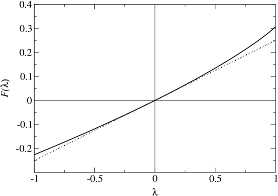
FIG. 1.: The function $F(\lambda)$. The dotted line is $F=\lambda/4$.

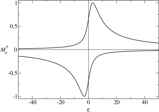
FIG. 2.: The mean field solutions $M_{\epsilon}^{+}$ (upper curve) and $M_{\epsilon}^{-}$ (lower curve).

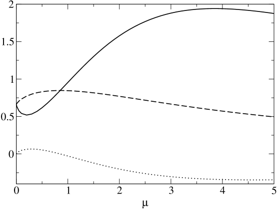
FIG. 3.: The integrals ${\cal J}$ (dashed curve) and ${\cal Y}$ (dotted curve), and the combination ${\cal J}-4{\cal Y}$ (solid curve), as functions of $\mu=m-4$.

REFERENCES

- [1] H. B. Nielsen and M. Ninomiya, Nucl. Phys. B185, 20 (1981); B193, 173 (1981).
- [2] For some recent reviews see H. Neuberger, hep-lat/0101006; M. Lüscher, hep-th/0102028; M. Golterman, Nucl. Phys. Proc. Suppl. 94, 189 (2001) [hep-lat/0011027]; R. Narayanan, hep-lat/0011017.
- [3] D. B. Kaplan, Phys. Lett. B 288, 342 (1992).
- [4] R. Narayanan and H. Neuberger, Phys. Lett. B 302, 62 (1993); Nucl. Phys. B412, 574 (1994); B443, 305 (1995); H. Neuberger, Phys. Lett. B 417, 141 (1998); 427, 353 (1998).
- [5] Y. Shamir, Nucl. Phys. B406, 90 (1993).
- [6] V. Furman and Y. Shamir, Nucl. Phys. B439, 54 (1995).
- [7] H. Neuberger, Phys. Rev. D 57, 5417 (1998).
- [8] P. M. Vranas, Phys. Rev. D 57, 1415 (1998).
- [9] Y. Kikukawa and T. Noguchi, hep-lat/9902022.
- [10] N. Kawamoto and J. Smit, Nucl. Phys. B 192, 100 (1981).
- [11] H. Kluberg-Stern, A. Morel, O. Napoly, and B. Petersson, Nucl. Phys. B 190, 504 (1981).
- [12] O. Martin, Phys. Lett. B 130, 411 (1983). O. Martin and B. Siu, ibid. 131, 419 (1983); R. Friedberg and O. Martin, Nucl. Phys. B 279, 684 (1987).
- [13] S. Myint and C. Rebbi, Nucl. Phys. B 421, 241 (1994) [hep-lat/9401009]; A. R. Levi, V. Lubicz, and C. Rebbi, Phys. Rev. D 56, 1101 (1997).
- [14] S. Aoki, Phys. Rev. D 30, 2653 (1984); 33, 2399 (1986); 34, 3170 (1986); Phys. Rev. Lett. 57, 3136 (1986).
- [15] I. Ichinose, Nucl. Phys. B 249, 715 (1985).
- [16] R. C. Brower and B. Svetitsky, Phys. Rev. D 61, 114511 (2000).
- [17] J. Smit, Nucl. Phys. B175, 307 (1980).
- [18] F. Berruto, G. Grignani, and P. Sodano, Phys. Rev. D 62, 054510 (2000).
- [19] M. Creutz, Rev. Mod. Phys. 50, 561 (1978); Quarks, gluons and lattices (Cambridge U. P., 1983).
- [20] R. Brower, P. Rossi and C. Tan, Nucl. Phys. B 190, 699 (1981).
- [21] R. C. Brower and M. Nauenberg, Nucl. Phys. B180, 221 (1981).
- [22] E. Brezin and D. J. Gross, Phys. Lett. B 97, 120 (1980).
- [23] B. Svetitsky, S. D. Drell, H. R. Quinn, and M. Weinstein, Phys. Rev. D 22, 490 (1980); M. Weinstein, S. D. Drell, H. R. Quinn, and B. Svetitsky, ibid. 22, 1190 (1980).
- [24] P. Hernandez, K. Jansen and M. Lüscher, Nucl. Phys. B 552, 363 (1999); H. Neuberger, Phys. Rev. D 61, 085015 (2000).
- [25] S. Aoki, T. Izubuchi, Y. Kuramashi and Y. Taniguchi, Phys. Rev. D 62, 094502 (2000) [hep-lat/0004003].
- [26] F. A. Berezin, Introduction to Superanalysis, (Reidel, Dordrecht, 1987); K. B. Efetov, Adv. Phys. 32, 53 (1983).
- [27] I. Ichinose and K. Nagao, Nucl. Phys. B577, 279 (2000); B596, 231 (2001).
- [28] M. Golterman and Y. Shamir, J. High Energy Phys. 0009, 006 (2000).