Abstract

Recent lattice data from CP-PACS, UKQCD, SESAM/TXL and the Pisa group regarding the quark mass dependence of the topological susceptibility in 2-flavour QCD are compared to each other and to theoretical expectations. The latter get specified by referring to the QCD finite-volume partition function with “granularity” which accounts for the entropy brought by instantons and anti-instantons. The chiral condensate in $N_{\!f}\!=\!2$ QCD, if determined by this method, turns out surprisingly large.

1 Introduction

Quenched QCD is, by many respects, a reasonable approximation to real (“full”) QCD; in particular for the light meson spectrum this approximation was found to work so well that a major effort had to be made to drive statistical errors small enough so that significant differences between the computed quenched and the experimentally observed (unquenched) spectrum could be seen [1]. On the other hand, there are observables which prove highly sensitive on quenching effects. An important example of this latter category is the topological susceptibility which, in the continuum, is defined, through [2]

$$\chi=\int\!d^{4}z\;\partial_{\mu}\partial_{\nu}\langle T\{k^{\mu}(x)k^{\nu}(y)\}\rangle\;,$$ (1)

where $z\!=\!x\!-\!y$ and

$$k^{\mu}(x)={g^{2}\over 16\pi^{2}}\epsilon^{\mu\nu\sigma\rho}A^{\mathrm{a}}_{\nu}(x)\Big{(}\partial_{\rho}A^{\mathrm{a}}_{\sigma}(x)-{g\over 3}f^{\mathrm{abc}}A^{\mathrm{b}}_{\rho}(x)A^{\mathrm{c}}_{\sigma}(x)\Big{)}$$ (2)

denotes the Chern current which is related to the topological charge density via

$$q(x)=\partial_{\mu}k^{\mu}(x)={g^{2}\over 32\pi^{2}}G^{\mathrm{a}}_{\mu\nu}(x)\tilde{G}^{\mathrm{a}\,\mu\nu}(x)\qquad\mathrm{with}\quad\tilde{G}^{\mu\nu}\!=\!{1\over 2}\epsilon^{\mu\nu\sigma\rho}G_{\sigma\rho}\;.$$ (3)

The topological susceptibility $\chi$ plays a prominent role in QCD, because its nonvanishing quenched counterpart $\chi_{\infty}$ explains through the Witten-Veneziano relation [2]

$$M_{\eta^{\prime}}^{2}-(2M_{K}^{2}-M_{\eta}^{2})={2N_{\!f}\over F_{\pi}^{2}}\chi_{\infty}$$ (4)

to leading order in $1/N_{\!c}$ why the $\eta^{\prime}$ is heavier than the octet of pseudoscalar mesons and hence not a pseudo-Goldstone. The topological susceptibility $\chi$ in the full theory is an interesting object to study unquenching effects, because it may deviate from the quenched prediction $\chi_{\infty}$ by up to 100%, if the dynamical quarks tend to be light. In this respect one should note that the dependence of $\chi\!=\!\chi(N_{\!f},m)$ on the number of dynamical quarks and their masses is not explicit in the definition (1); it enters implicitly via the vacuum expectation value $\langle...\rangle$ which includes the weight of the fermion functional determinant. This means that the topological susceptibility is useful to study the QCD vacuum structure and how the latter is affected by the presence of light dynamical quarks. It is therefore little surprise that the first reliable lattice data for the topological susceptibility in full QCD were eagerly awaited for.

Below we shall analyze the data by CP-PACS [3], UKQCD [4], SESAM/TXL [5] and the Pisa group [6]. We will see that they are roughly consistent with each other, but follow theoretical expectations to a limited extent only. Potential sources of error are analyzed, and it is shown that specifically for the topological susceptibility finite-volume effects may be quantitatively assessed by deriving it from the QCD finite-volume partition function for which an elaborate version is given. On the practical side, a non-standard determination of the chiral condensate in $N_{\!f}\!=\!2$ QCD is presented, and the result is found surprisingly large.

2 Theoretical expectations

To begin, we shall remind ourselves of the theoretical expectations regarding the dependence of the topological susceptibility $\chi$ on the sea-quark masses $m_{1},\ldots,m_{N_{\!f}}$. For simplicity the latter shall be taken degenerate, i.e. we are interested in the function $\chi\!=\!\chi(N_{\!f},m)$ with $N_{\!f}\!\geq\!2$. In the present section the four-volume $V$ of the box is assumed “infinite”; finite-volume effects will be analyzed below.

Detailed predictions on $\chi\!=\!\chi(N_{\!f},m)$ may be obtained for the two regimes where the quark masses tend to be either very light or very heavy. In the former case the flavour singlet axial Ward-Takahashi (WT) identity dictates that $\chi$ raises linearly [7, 8, 9], viz.

$$\chi={\Sigma\over N_{\!f}}\,m+o(m)\;,$$ (5)

where $\Sigma\!=\!-\lim_{m\to 0}\lim_{V\to\infty}\langle\overline{\psi}\psi\rangle$ is the chiral (one-flavour) condensate in the chiral limit and the $o(m)$ term contains higher order corrections which may be worked out explicitly in chiral perturbation theory [10]. On the other hand, for heavy dynamical quarks the topological susceptibility curve will be almost flat, because it must gradually approach the quenched value $\chi_{\infty}$ which is finite. A numerical estimate of the latter quantity by means of the Witten-Veneziano relation (4) yields $\chi_{\infty}\!\simeq\!(180\,\mathrm{MeV})^{4}\!\simeq\!1.05\;10^{9}\,\mathrm{MeV}^{4}$. In addition, it is easy to come up with plausible arguments that $\chi$ grows monotonically as the quark mass increases and that the second derivative is negative ².

Figure 1: Basic illustrations regarding the topological susceptibility [in $\mathrm{MeV}^{4}$] versus the quark mass [in $\mathrm{MeV}$] for 2-flavour QCD with $\Sigma\!=\!(288\,\mathrm{MeV})^{3}$ (cf. footnote 5). LHS: The leading order chiral prediction in the large Leutwyler-Smilga regime without instanton effects (5) (raising slope) and the quenched prediction from the Witten-Veneziano relation (4) (flat line). RHS: The curves with $n\!=\!1,2,4,8$ (from the lowest to the highest) out of the phenomenological family (6), all of which share the required asymptotic behaviour.

Hence, without doing a detailed analysis, a clear picture emerges for the qualitative behaviour of the topological susceptibility as a function of the quark mass over the whole range of the latter. Even the transition regime may be estimated by just equating the leading-order chiral expression (5) to the asymptotic value $\chi_{\infty}$, as is illustrated on the l.h.s. of Fig. 1: Upon using $\Sigma\!=\!(288\,\mathrm{MeV})^{3}\!=\!2.4\;10^{7}\,\mathrm{MeV}^{3}$ one gets $m_{\mathrm{trans}}\!\simeq\!88\,\mathrm{MeV}$ for 2-flavour QCD, which is accessible in current dynamical simulations.

What these considerations cannot yield is the functional form of the topological susceptibility curve. Of course it is easy to come up with a whole bunch of phenomenological models or ansätze which interpolate in various ways between the asymptotic regimes; e.g.

$$\chi(N_{\!f},m)=((\Sigma\;m/N_{\!f})^{-n}+\chi_{\infty}^{-n})^{-1/n}$$ (6)

is a one-parameter family of interpolating curves (some of which are displayed in the r.h.s. of Fig. 1) with the required asymptotic behaviour.

In summary, one would expect up-to-date simulations of full 2-flavour QCD to show the turn-over from a linear to an almost flat behaviour at a quark mass of $O(88\,\mathrm{MeV})$, and to select the most promising phenomenological overall fitting curve from the set (6).

3 Lattice data

Before considering the actual data, we should remind ourselves that it is not the original definition (1) of the topological susceptibility which is typically used on the lattice, but a simplified version which – at least in the continuum – proves equivalent.

The simplification takes place as the result of a two-step procedure. The first step is to assume translation invariance of the vacuum, so (1) simplifies to

$$\chi=\int\!d^{4}x\;\langle T\{q(x)q(0)\}\rangle\;,$$ (7)

where we have also assumed that the $\delta$-functions due to the derivatives in (1) hitting the $T$-ordering do not contribute after integration. The second step assumes that there is, in addition, no correlation between topological charge densities, so (7) simplifies to

$$\chi={\langle q^{2}\rangle\over V}\;,$$ (8)

where

$$q={g^{2}\over 32\pi^{2}}\int\!d^{4}x\;G^{\mathrm{a}}_{\mu\nu}\tilde{G}^{\mathrm{a}\;\mu\nu}$$ (9)

is the (global) topological charge which, in the continuum, takes an integer value. The important point is that the original definition (1) provides a detailed prescription of how to deal with the $\delta$-like singularity in the product $q(x)q(0)$ which is not explicit any more in the simplified version (8). As a matter of consequence [12], a lattice implementation of (1) is subject to a multiplicative renormalization only

$$\hat{\chi}=Z^{2}\,a^{4}\,\chi+O(a^{6})$$ (10)

with the renormalization factor of the topological charge

$$\hat{q}=Z\,q+O(a^{2})\;,$$ (11)

whereas a lattice version of (8) shows an additional additive renormalization, viz.

$$\hat{\chi}=M(\beta,N_{\!f},m)+Z^{2}\,a^{4}\,\chi+O(a^{6})\,.$$ (12)

While in practice both the multiplicative renormalization factor $Z$ and the additive piece $M$ do not cause any difficulties, since they may be determined by means of heating techniques [13], an explicit verification of the three definitions (1, 7, 8) proving equivalent after they have been implemented on the lattice is still being awaited. Since, as we have seen, proper treatment of contact terms is essential in this game (cf. [14] and references therein), such an investigation might be interesting in its own right.

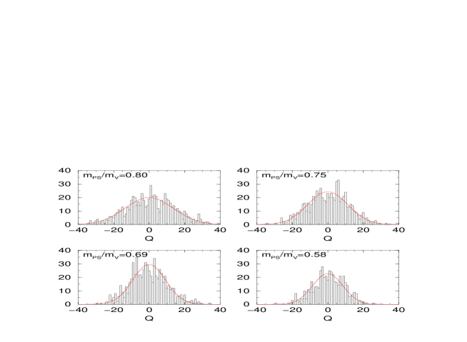
Figure 2: CP-PACS data for the distribution of topological charges on a $16^{3}\!\times\!32$ lattice after cooling with an RG-improved action. The configurations were generated using the same (Iwasaki) action at fixed $\beta\!=\!1.95$ together with 2 flavours of mean-field improved clover quarks ($c_{{}_{\mathrm{SW}}}\!=\!1.53$) at 4 different $\kappa$-values. Figure by courtesy of the CP-PACS collaboration.

After these cautionary remarks we are ready to esteem the latest lattice data which use the simplified definition (8), thereby dealing – in principle – with the renormalization pattern (12). In order to get a feeling of what is actually done, it is useful to consider the distribution of topological charges as found by the CP-PACS collaboration [3]. Fig. 2 shows the histograms they have gotten on a $16^{3}\!\times\!32$ lattice at $\beta\!=\!1.95$ (using the Iwasaki action) and at four different $\kappa$-values ($\kappa\!=\!0.1375,0.1390,0.1400,0.1410$, giving $M_{\pi}/M_{\rho}\!=\!0.80,0.75,0.69,0.58$, respectively) for 2 flavours of mean-field improved clover quarks ($c_{{}_{\mathrm{SW}}}\!=\!1.53$) after cooling with the Iwasaki action and binning $q$ to integer values.

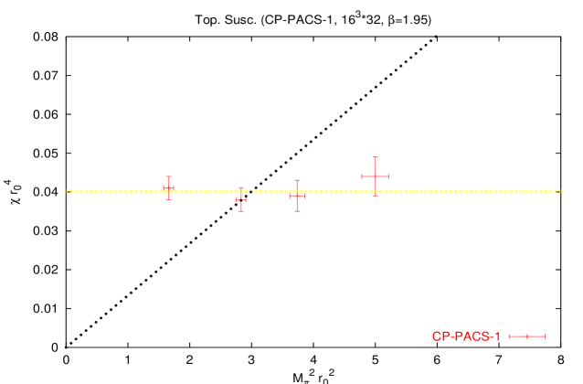
Figure 3: CP-PACS data for the topological susceptibility [in units of $r_{0}^{-4}$] versus the quark mass [expressed in terms of $M_{\pi}^{2}r_{0}^{2}$] in 2-flavour QCD, as determined from the $q$-distributions shown in Fig. 2. The linearly raising slope indicates the asymptotic behaviour for light dynamical quarks ($\chi_{0}r_{0}^{4}\!\simeq\!(F_{\pi}^{2}r_{0}^{2}/2N_{\!f})M_{\pi}^{2}r_{0}^{2}\!\simeq\!0.0133\,M_{\pi}^{2}r_{0}^{2}$ for $F_{\pi}\!\simeq\!93\,\mathrm{MeV}$ and $r_{0}\!\simeq\!0.49\,\mathrm{fm}$), and the horizontal line the one for (infinitely) heavy dynamical quarks ($\chi_{\infty}r_{0}^{4}\!\simeq\!(180\,\mathrm{MeV})^{4}\,(0.49\,\mathrm{fm})^{4}\!\simeq\!0.04$), as in the l.h.s. of Fig. 1. The data are expected to lie in the sector beneath either one of these lines, i.e. $\chi r_{0}^{4}\!\leq\!\mathrm{min}(\chi_{0}r_{0}^{4},\chi_{\infty}r_{0}^{4})$, where $\chi_{\infty}$ might be somewhat larger (cf. text). Data taken from [3, 9].

Since the cooling procedure brings both renormalization constants ($Z$ and $M$) close to their continuum values ($1$ and $0$, respectively), one can basically read off the expectation values $\langle q^{2}\rangle$ from the widths of the distributions shown in Fig. 2. This holds, because

$$\langle q^{2}\rangle\equiv{\int\!dq\;q^{2}\;e^{-q^{2}/2\sigma^{2}}\over\int\!dq\;e^{-q^{2}/2\sigma^{2}}}=\sigma^{2}$$ (13)

for a gaussian distribution. Hence, from a glimpse at Fig. 2 one might get the impression that the topological susceptibility gets reduced as the quark mass decreases, since the $q$-distribution does indeed get narrower as $\kappa$ increases. What this naive consideration neglects is that the topological susceptibility $\chi$ is defined as the variance of these gaussian curves divided by the physical four-volume of the box (cf. (8, 13)), and the latter changes with $\kappa$, because in full QCD the physical lattice spacing $a$ is a non-trivial function of $\beta$ and $\kappa$. To be specific: $a$ decreases if $\kappa$ gets increased at fixed $\beta$, and for the volume the reduction is particularly strong, as it involves the fourth power of $a$. Taking this effect into account yields the data for $\chi$ versus the dynamical quark mass $m$ in $N_{\!f}\!=\!2$ QCD shown in Fig. 3. They seem to indicate an almost flat topological susceptibility curve, and this means that the narrowing of the $q$-distribution in Fig. 2 was exclusively due to the volume $V$ decreasing with increasing $\kappa$ (at fixed $\beta$) and not due to a decrease of $\chi$. In other words: The data in Fig. 3 show no sign of the expected transition to the linear behaviour (5) characteristic for light dynamical quarks, even though the most chiral point is at $M_{\pi}^{2}r_{0}^{2}\!=\!1.66$, i.e. at a quark mass of $m\!\simeq\!50\mathrm{MeV}$ (using $F_{\pi}\!=\!93\,\mathrm{MeV},\Sigma\!=\!(288\,\mathrm{MeV})^{3}$) which is well below our estimate of the transition regime; we had $m_{\mathrm{trans}}\!\simeq\!88\,\mathrm{MeV}$ for $N_{\!f}\!=\!2$. The troublesome point is the most chiral one; it seems to violate the constraint $\chi\!\leq\!\chi_{0}$ with $\chi_{0}$ defined as the r.h.s. of (5). Potential reasons for the supposed excess of the measured $\hat{\chi}$ will be discussed below.

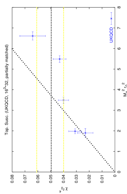
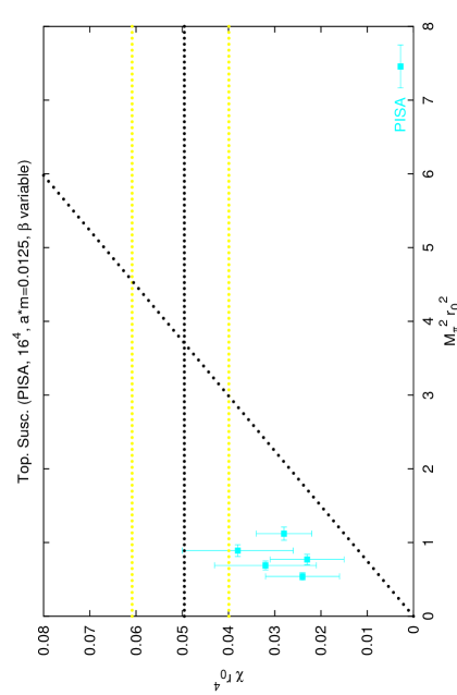
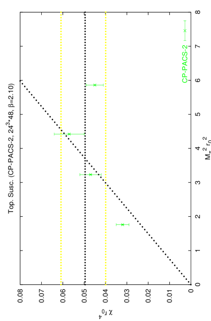
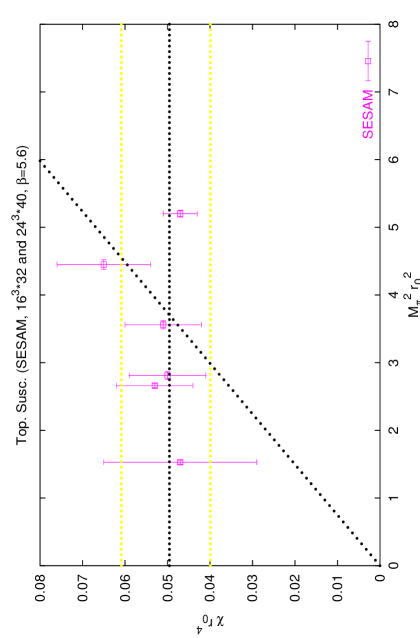
Figure 4: Data for the topological susceptibility versus the quark mass in $N_{\!f}\!=\!2$ QCD by CP-PACS, UKQCD, SESAM and the Pisa group. The two asymptotic constraints (based on $F_{\pi}\!=\!93\,\mathrm{MeV}$ and $\chi_{\infty}\!=\!(190\!\pm\!10\,\mathrm{MeV})^{4}$, respectively) are shown; the data are supposed to lie beneath either line, i.e. in the lower right sector (for details see text). Data taken from [3, 4, 5, 6, 9].

From Fig. 4 one sees that the data generated by the CP-PACS collaboration on the larger lattice ($24^{3}\!\times\!48$ at $\beta\!=\!2.10$) as well as the results obtained by UKQCD and the Pisa group are “better” in the sense that they barely support an entirely flat behaviour, but they still seem to be at the edge of being compatible with the constraints imposed by the known asymptotic behaviour for small quark masses. For the CP-PACS data at $\beta\!=\!2.10$ and the UKQCD data the hypothesis that the true 2-flavour topological susceptibility curve lies in the sector beneath either one of the two indicated lines seems conceivable, in particular if one takes into account that the horizontal line itself is subject to some uncertainty. The remaining constraints – the first derivative of $\chi(m)$ must always be positive, the second always negative – seem to be obeyed with the (unsignificant) exception of one point in each one of these two simulations. Thanks to relatively large error bars, it seems that the data obtained by the SESAM-collaboration are at the edge of being compatible with the two asymptotic constraints. For the data due to the Pisa group the situation looks less promising: Each one of their data points is compatible, on a $2\sigma$-level, with the linear constraint applicable in the deep chiral regime, but the combination of the five points is not. For obvious reasons nothing can be said about the first two derivatives from either the SESAM or the Pisa data, the error bars are just too large.

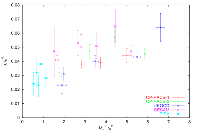
Figure 5: Collection of recently published data for the topological susceptibility in $N_{\!f}\!=\!2$ QCD.

Another simple cross-check is to combine the results obtained by the various collaborations in a single plot and to see whether there is an obvious trend for the data to depend on the group, an endeavour undertaken in Fig. 5. The first impression is that the data are vaguely consistent with each other, but even for the combined data it is not clear whether they show all of the transient behaviour we expect to see with active flavours which are neither light enough to produce a linear curve through the origin nor heavy enough to have the topological susceptibility flatten out at the saturated quenched level: They seem to indicate a positive slope (though the band is rather fuzzy), but it is not clear whether the combined data do exhibit the negative curvature genuine to the transition region anticipated at $m\!=\!O(88\mathrm{MeV})$ or $M_{\pi}^{2}r_{0}^{2}\!=\!O(3)$ for $N_{\!f}\!=\!2$ (cf. Fig. 1).

CP-PACS-1	$16^{3}\times 32$	$\beta\!=\!1.95$	$c_{{}_{\mathrm{SW}}}\!\!=\!\!1.53$
$\kappa$	0.1410	0.1400	0.1390	0.1375
$M_{\pi}/M_{\rho}$	0.586	0.688	0.751	0.805
$M_{\pi}^{2}r_{0}^{2}$	1.66	2.83	3.74	5.00
$\chi r_{0}^{4}$	0.041	0.038	0.039	0.044
$a_{\sigma}[\mathrm{fm}]$	0.170	0.181	0.193	0.204
$V[\mathrm{fm}^{4}]$	109.	141.	182.	227.
$x\!\equiv\!V\Sigma m$	42.0	92.1	157.	263.

CP-PACS-2	$24^{3}\times 48$	$\beta\!=\!2.10$	$c_{{}_{\mathrm{SW}}}\!\!=\!\!1.47$
$\kappa$	0.1382	0.1374	0.1367	0.1357
$M_{\pi}/M_{\rho}$	0.575	0.690	0.757	0.806
$M_{\pi}^{2}r_{0}^{2}$	1.76	3.23	4.44	5.86
$\chi r_{0}^{4}$	0.032	0.047	0.057	0.045
$a_{\sigma}[\mathrm{fm}]$	0.113	0.120	0.126	0.134
$V[\mathrm{fm}^{4}]$	107.	138.	167.	215.
$x\!\equiv\!V\Sigma m$	43.7	103.	171.	292.

UKQCD	$16^{3}\times 32$	partially	matched
$\beta$	5.20	5.20	5.20	5.26	5.29
$c_{{}_{\mathrm{SW}}}$	2.02	2.02	2.02	1.95	1.92
$\kappa$	0.13565	0.1355	0.1350	0.1345	0.1340
$M_{\pi}/M_{\rho}$	0.567	0.600	0.688	0.791	0.830
$M_{\pi}^{2}r_{0}^{2}$	1.90	1.98	3.49	5.49	6.61
$\chi r_{0}^{4}$	0.023	0.031	0.040	0.043	0.064
$a_{r_{0}}[\mathrm{fm}]$	0.094	0.097	0.103	0.104	0.102
$V[\mathrm{fm}^{4}]$	10.3	11.7	14.8	15.4	14.1
$x\!\equiv\!V\Sigma m$	9.1	10.7	23.9	39.1	43.1

SESAM	$16^{3}\times 32$	$\beta\!=\!5.6$	$c_{{}_{\mathrm{SW}}}\!\!=\!\!0$		$24^{3}\times 40$	dito
$\kappa$	0.1575	0.1570	0.1565	0.1560	0.1580	0.1575
$M_{\pi}/M_{\rho}$	0.692	0.763	0.813	0.834	0.574	0.704
$M_{\pi}^{2}r_{0}^{2}$	2.81	3.56	4.45	5.20	1.53	2.66
$\chi r_{0}^{4}$	0.050	0.051	0.065	0.047	0.047	0.053
$a_{r_{0}}[\mathrm{fm}]$	0.084	0.091	0.095	0.098	0.080	0.085
$V[\mathrm{fm}^{4}]$	6.5	9.1	10.6	12.1	23.1	28.9
$x\!\equiv\!V\Sigma m$	8.5	15.1	21.8	29.1	16.4	35.6

PISA	$16^{4}$	$am\;=\!$	$\!\!0.0125$	($N_{\!f}\!=\!2$	stag.)
$\beta$	5.40	5.50	5.55	5.60	5.70
$M_{\pi}^{2}r_{0}^{2}$	0.54	0.69	0.77	0.89	1.12
$\chi r_{0}^{4}$	0.024	0.032	0.023	0.038	0.028
$a_{\sigma}[\mathrm{fm}]$	0.174	0.134	0.125	0.108	0.086
$V[\mathrm{fm}^{4}]$	60.3	21.3	15.9	8.78	3.55
$x\!\equiv\!V\Sigma m$	15.1	6.8	5.7	3.6	1.8

Tables 1-5: Key data of the five studies. For error bars see Figs. 1-5 and Refs. [3, 4, 5, 6, 9]. In all cases the Leutwyler-Smilga parameter $x\!\equiv\!V\Sigma m$ has been estimated by re-expressing it, through the GOR relation, as $x\!=\!VM_{\pi}^{2}F_{\pi}^{2}/2\!=\!V(M_{\pi}^{2}r_{0}^{2})(F_{\pi}^{2}/2r_{0}^{2})$ with $F_{\pi}\!\simeq\!93\,\mathrm{MeV},r_{0}\!\simeq\!0.49\,\mathrm{fm}$.

The consistency between the various data sets cannot be discussed, however, without taking into account that the groups have adopted rather different simulation strategies. CP-PACS has decided to simulate at fixed $\beta$, going more chiral by tuning $\kappa$ closer to $\kappa_{\mathrm{crit}}$. As discussed above, this approach reduces the physical lattice spacing $a$ for low $M_{\pi}/M_{\rho}$. In order to keep $a$ constant, one would have to reduce $\beta$ appropriately while increasing $\kappa$, an approach which – if successfully implemented – produces “matched ensembles”. This is the philosophy adopted by UKQCD. For technical reasons ($c_{{}_{\mathrm{SW}}}$ is not known nonperturbatively for $\beta\!<\!5.2$) this strategy had to be sacrificed for their two most chiral points, i.e. their data set is, strictly speaking, just “partially matched”. SESAM, on the other hand, has decided to take everywhere the simplest choice, i.e. to vary $\kappa$ at fixed $\beta$ while not making any attempt to improve the Wilson fermions. An orthogonal strategy has been adopted by the Pisa group: They simulate (using the staggered rather than a Wilson-type formulation for their dynamical flavours) at fixed $am$, thus decreasing $\beta$ in order to go more chiral. Note that – contrary to what happens in a series of fixed-$\beta$ simulations – the Pisa approach makes the lattice coarser as one goes more chiral.

A possible inconsistency between the results by the different groups could come from a variety of reasons:

(a) Scaling violations: Because of the computational costs involved in full QCD simulations the latter are typically performed on relatively coarse lattices (cf. Tables 1-5). For the simulations analyzed in this article scaling violations are supposed to be “small” since $O(a)$ effects have been removed by mean-field techniques (CP-PACS) or non-perturbatively (UKQCD) or they might be numerically suppressed due to a small $a$ (SESAM) or absent anyway (Pisa group). Nontheless, the physical lattice spacing varying from one data point to another in the same study might imply unequal shifts due to cutoff effects.

(b) Chirality violation with Wilson-type fermions: Wilson fermions (SESAM) violate the chiral symmetry at nonzero lattice spacing, and this holds true, too, for all ultralocally improved descendents (e.g. the clover-fermions used by CP-PACS and UKQCD).

(c) Finite-volume effects: From Tables 1-5 one learns that the five studies have been conducted in boxes of rather different physical four-volume $V$ and at rather different values of the Leutwyler-Smilga parameter $x\!\equiv\!V\Sigma m$. Hence, if finite-volume effects are not fully under control, potential inconsistencies of type (a) or (b) might get masked by them.

I have a few comments on each one of these points:

On (a): UKQCD claimed that in order to get simulation results which indicate a quark mass dependence of the topological susceptibility it was crucial to use the strategy of generating matched ensembles, rather than running at fixed $\beta$ [4]. Despite this assertion it holds true that in principle either method should work: If one could do both a continuum and a chiral extrapolation, it should not matter at all where in the $(\beta,\kappa)$ plane the data were collected. In practice a continuum extrapolation at fixed quark mass is unaffordable at the present time, and hence each group has to live with the single data point for a given value of $M_{\pi}^{2}r_{0}^{2}$. Since both UKQCD and CP-PACS work with $O(a)$ improved actions for which a continuum extrapolation was shown to bring just a minor shift in the case of pseudoscalar masses [9], it is natural to expect the topological susceptibility data to be reasonably close to their continuum values too. If unequal magnitudes of scaling violations in a fixed-$\beta$ strategy were indeed responsible for the majority of the CP-PACS-1 “flatness problem”, then one would expect the data generated by CP-PACS at $\beta\!=\!1.95$ to be subject to larger shifts for large quark masses (where the lattice is coarser) versus more trustworthy at small quark masses (where $a$ is smaller), but from Fig. 3 one gets the impression that the problem with that particular set is primarily in its most chiral point. Scaling violations may indeed account for the bulk of the difference between the UKQCD and CP-PACS-1 data sets, but it seems that such a difference is much more likely associated with the respective overall differences between typical lattice spacings (Tables 1 and 3 indicate that UKQCD works on much finer lattices than those employed by CP-PACS at $\beta\!=\!1.95$) rather than whether these sets are matched or not. This is also the conclusion one is led to when comparing the CP-PACS-1 data (Table 1) to those entitled CP-PACS-2 (Table 2): The latter seem to indicate a quark mass dependence even though they were generated at fixed $\beta\!=\!2.10$. Since the volume parameters $V$ and $x$ are in one-to-one analogy between CP-PACS-1 and CP-PACS-2 (see Tables 1 and 2), the only difference is the lattice spacing which is significantly smaller at the higher $\beta$-value.

On (b): The quark mass dependence of the topological susceptibility in the extreme chiral regime is derived from the flavour singlet axial WT-identity. With Wilson quarks (or descendents which do not satisfy the Ginsparg-Wilson relation) this identity receives additional terms [15]. This may result in the lattice topological susceptibility $\hat{\chi}$ being enhanced compared to its continuum counterpart $\chi$. It should be mentioned, however, that this effect is, in principle, accounted for by the additive renormalization term in (12). Hence, on a practical level, an accurate determination of $M\!=\!M(\beta,N_{\!f},m)$ should be sufficient to deal with this challenge.

On (c): As indicated in footnote 2, for the topological susceptibility to raise linearly as a function of the (small) quark mass it is important that the volume is “infinite”, i.e. in more technical terms that the Leutwyler-Smilga parameter (14) is large. How “large” it has to be for this behaviour to show up and what pattern the topological susceptibility follows if this criterion is not satisfied will be discussed in the following two sections. As we shall see, finite-volume effects are the only source of contamination of the lattice topological susceptibility for which an a-priory quantitative assessment may be achieved.

4 Leutwyler-Smilga regimes

Considering a theory which exhibits the spontaneous breakdown of a continuous global symmetry (e.g. of the $SU(N_{\!f})_{A}$ group for QCD) in a finite volume, one expects to see both symmetry restoration phenomena and the onset of Goldstone boson production, if the box is taken sufficiently “small” or “large”, respectively. An obvious question is what sets the scale, i.e. by which standards does the box have to be small or large to trigger one or the other type of phenomena ?

The naive guess is the lightest particle at hand, i.e. the mass $M_{\pi}$ of the pseudo-Goldstone boson produced in the infinite-volume limit. From this one would expect symmetry restoration to take place for $M_{\pi}L\!\ll\!1$ and SSB to become manifest for $M_{\pi}L\!\gg\!1$.

As Leutwyler and Smilga (LS) have shown [8], there is, in addition, the parameter

$$x\equiv V\Sigma m$$ (14)

which also depends on the quark mass and which proves particularly useful in a lattice context, since it decides which one of the limits $m\!\to\!0,V\!\to\!\infty$ is in the “inner” position and therefore winning. In other words: For $x\!\ll\!1$ the chiral symmetry is almost restored, i.e. quarks and gluons are the dominant degrees of freedom, whereas for $x\!\gg\!1$ the chiral symmetry is (though the box volume is still finite) effectively broken, i.e. long range Green’s functions are dominated by Goldstone excitations. Furthermore, the value of $x$ has a bearing on whether standard physical observables depend on the net topological charge $q$ of the gauge background or not [8]: In the small LS-regime ($x\!\ll\!1$) all observables depend massively on $|q|$, and the finite-volume partition function is entirely dominated by the contribution from the charge zero sector [8], viz.

$$Z_{\nu}\simeq\delta_{\nu\,0}\qquad\qquad(x\!\ll\!1)\;.$$ (15)

On the other hand, in the large LS-regime ($x\!\gg\!1$) standard observables prove basically independent of $|q|$ (for a numerical check and some qualifications see [16]), and the finite-volume partition function gets broad and gaussian [8], viz.

$$Z_{\nu}\simeq{1\over\sqrt{2\pi\sigma^{2}}}\exp\{-{\nu^{2}\over 2\sigma^{2}}\}\quad,\qquad\sigma^{2}={V\Sigma m\over N_{\!f}}\qquad\qquad(x\!\gg\!1)\;.$$ (16)

It is important to note that the LS-parameter $x$ and the “naive” parameter

$$y\equiv M_{\pi}L$$ (17)

are not the same: In either one of the regimes with pronounced ($x\!\gg\!1$) or mild ($x\!\simeq\!1$) SSB the box may be large ($y\!\gg\!1$), intermediate ($y\!\simeq\!1$) or even small ($y\!\ll\!1$) w.r.t. the pion correlation length classification, whereas in the symmetry restoration regime ($x\!\ll\!1$) such a distinction does not make sense, since there the pion is not a useful degree of freedom. That $x$ and $y$ cover different aspects of the box being “small” or “large” is also borne out by the fact that the minimum box length scales differently as a function of the inverse quark mass, if one wants the box to be large w.r.t. either criterion, i.e.

$$L_{\mathrm{\min}}\propto(1/m)^{1/4} \mathrm{for} m\to 0\;\mathrm{at}\;\mathrm{fixed}\;(\mathrm{large})\;x$$ (18)

$$L_{\mathrm{\min}}\propto(1/m)^{1/2} \mathrm{for} m\to 0\;\mathrm{at}\;\mathrm{fixed}\;(\mathrm{large})\;y,$$ (19)

which simply follows from the definition (14) of $x$ and the GOR relation, respectively. Furthermore, it is worth noticing that in a lattice context the LS-classification refers to the mass of the sea-quarks (i.e. the dynamical quarks which influence the weight of a gauge configuration through the determinant), whereas the conventional one refers to the mass of the current-quarks (i.e. those from which hadronic observables are built).

In QCD the chiral symmetry restoration transition is intricately related to the deconfinement transition, and this is the reason why even the combination of the parameters $x$ and $y$ is not sufficient to describe the broad properties of the finite-volume system. This is easily seen from the fact that the confinement-deconfinement transition takes place at a critical temperature $T_{c}\!\simeq\!275\,\mathrm{MeV}$ in pure $SU(3)$-gluodynamics and at a somewhat reduced temperature $T_{c}\!\simeq\!175\,\mathrm{MeV}$ in QCD with $N_{\!f}\!=\!2$ massless flavours. In other words: $T_{c}$ stays at the same order of magnitude while both $x$ (cf. (14)) and $y$ (cf. 17)) decrease from infinity to zero as the quarks are tuned from infinitely heavy to weightless. Hence a third scale must be involved which – contrary to $x$ and $y$ – barely depends on $N_{\!f}$ and $m$. It is tempting to identify the missing scale with the one due to instantons, i.e. to introduce the parameter

$$z\equiv{L_{\mathrm{min}}\over L_{\mathrm{inst}}}$$ (20)

where $L_{\mathrm{min}}$ is the smallest linear dimension of the box, and $L_{\mathrm{inst}}$ is a typical linear size associated to an instanton, e.g. $L_{\mathrm{inst}}\!=\!2\rho_{\mathrm{inst}}\!\simeq\!0.7\,\mathrm{fm}$ or $L_{\mathrm{inst}}\!=\!V_{\mathrm{inst}}^{1/4}\!\simeq\!1\,\mathrm{fm}$ [18], since such a scale is, to a large extent, independent of the number and mass of the active flavours. For $z\!\ll\!1$ the system is in the deconfined state, i.e. quarks and gluons represent the appropriate degrees of freedom, whereas for $z\!\gg\!1$ confinement is manifest, i.e. asymptotic states are colour singlets, and the associate composite fields are the building blocks of the effective description appropriate in that regime.

As we shall see in the following section, the subtle interplay between the LS-scale $x$ (which depends on the quark masses) and the instanton size (which barely does) is crucial for an understanding of the overall behaviour of the topological susceptibility curve in QCD.

5 Finite-volume partition function with “granularity”

We are now in a position to exploit the fact that one may actually derive the topological susceptibility from the finite-volume partition function, and for the latter several versions are available in the literature.

In the large LS-regime the situation is particularly simple, since from the representation (16) of the QCD finite-volume partition function one gets $\langle\nu^{2}\rangle\!=\!V\Sigma m/N_{\!f}$ and hence the linearly raising behaviour (5) of the topological susceptibility, valid for $x\!\gg\!1$. Analogously, one may compute $\chi$ from $Z_{\nu}$ in the other two regimes, since Leutwyler and Smilga give, in their landmark paper [8], also the generalization of (16) to arbitrary $x$:

$$Z_{\nu}^{\mathrm{XPT}}=\left|\begin{array}[]{cccc}I_{\nu}(x)&I_{\nu+1}(x)&\cdots&I_{\nu+N_{\!f}-1}(x)\\ I_{\nu-1}(x)&I_{\nu}(x)&\cdots&I_{\nu+N_{\!f}-2}(x)\\ \vdots&\vdots&\ddots&\vdots\\ I_{\nu-N_{\!f}+1}(x)&I_{\nu-N_{\!f}+2}(x)&\cdots&I_{\nu}(x)\end{array}\right|\;.$$ (21)

It is easy to check that, upon using the asymptotic form $I_{\nu}(x)\!\simeq\!e^{x}(1-(\nu^{2}\!-\!1)/(8x))/\sqrt{2\pi x}$ for $x\!\gg\!1$ of the modified Bessel function of integer order, the representation (21) of the partition function reduces to (16) for $x\!\gg\!1$, hence reproducing the linearly raising form (5) of $\chi$ in the large LS-regime. Furthermore, from the representation $I_{\nu}(x)\!\simeq\!x^{|\nu|}/(2^{|\nu|}\Gamma(|\nu|\!+\!1))$ appropriate in the opposite case $x\!\ll\!1$ one gets the asymptotic behaviour [8]

$$\chi\propto m^{N_{\!f}}\qquad\qquad(x\!\ll\!1)$$ (22)

characteristic for the small LS-regime. For an $x$ value which is neither small nor large compared to one, a numerical evaluation of $\langle\nu^{2}\rangle\!=\!\Sigma\nu^{2}Z_{\nu}^{\mathrm{XPT}}/\Sigma Z_{\nu}^{\mathrm{XPT}}$ is needed, and the result may be compared to the asymptotic behaviour (5) or (22) for $x\!>\!1$ or $x\!<\!1$. One of these comparisons is demonstrated on the l.h.s. of Fig. 6. There are two important lessons we can learn from that graph. First, finite-volume effects have a decreasing effect on the topological susceptibility. Second, the topological susceptibility as derived from (21) and the large-$x$ asymptotic form (5) are reasonably close for moderate $x$-values already. To be definite: For $V\!=\!10.125\,\mathrm{fm}^{4}$ and $\Sigma\!=\!(288\,\mathrm{MeV})^{3}$, the mark $x\!=\!1$ is reached at a quark mass $m\!=\!6.26\,\mathrm{MeV}$, and there the finite-$x$ value is about 50% smaller than the asymptotic prediction. Taking the quark mass 10 times larger, $m\!=\!62.6\,\mathrm{MeV}$ (i.e. $x\!=\!10$), the finite-$x$ value lies less than 10% below the asymptotic (large-$x$) prediction (cf. Fig. 6).

Figure 6: LHS: Topological susceptibility (without instanton effects) [in $\mathrm{MeV}^{4}$] versus quark mass [in $\mathrm{MeV}$] as derived from (21) (full curve), and the large-$x$ asymptotic form (5) (dashed line) in a box of $V\!=\!2\,(1.5\,\mathrm{fm})^{4}$ with $\Sigma\!=\!(288\,\mathrm{MeV})^{3}$. Since $N_{\!f}\!=\!2$, the small-$x$ asymptotic form is a parabola (cf. (22)). RHS: Illustration of the scenario in which the topological susceptibility in a finite volume (full) “overshoots” the infinite-volume curve (dashed) for some intermediate quark masses, hence explaining the CP-PACS “flatness problem” showing up in Fig. 3. In this illustration, the “granularity” of the QCD vacuum, as discussed in the text, is already taken into account. This “overshooting” scenario is excluded, since finite volume effects may only have a decreasing effect on $\chi$ (cf. LHS and the “granular” construction (27) discussed in the text).

The first statement is important, because it rules out a possible explanation of the “flatness problem” in the CP-PACS determination of the topological susceptibility on the smaller ($16^{3}\!\times\!32,\beta\!=\!1.95$) lattice, apparent in Fig. 3: Knowing that the topological susceptibility drops, in the small LS-regime, with a power-like behaviour – cf. (22) – and thus stays massively below the linear curve (5), one might have suspected that $\chi$ could “overshoot” and lie above the linear curve in an intermediate regime. Such a hypothetical behaviour, as illustrated in the r.h.s. of Fig. 6, which would provide a simple explanation why the leftmost point in Fig. 3 is so high, is definitely ruled out by the graph on the l.h.s. of Fig. 6; in other words, the “chiral constraint” indicated in Figs. 3 and 4 is to be taken seriously.

The second statement is important, because it implies that in a lattice study the minimum box length needed to avoid finite-volume effects in the topological susceptibility is much smaller than what one might have suspected by analogy with the standard pion correlation length criterion. The standard criterion says that in the broken phase the minimum box length $L_{\mathrm{min}}$ has to be larger than $\xi_{\pi}$ by up to a factor 4 to avoid finite-volume effects in hadronic Green’s functions. If the same factor (per linear dimension) would be relevant for the LS-parameter $x$, the latter would have to be of order $4^{4}\!=\!256$, which, as one can see from Tables 1-5, is hardly the case in any of the simulations discussed in this article. Hence from the l.h.s. of Fig. 6 one takes the good news that the actual value needed is much smaller; already $x\!\geq\!10$ seems sufficient to make the curve lie reasonably close to the large-$x$ line. Furthermore, comparing $\chi$ as predicted by the QCD partition functions (16) and (21) offers the potential benefit to quantify finite-volume effects in the topological susceptibility.

The next step is to recall that there is an important limitation to either topological susceptibility curve shown in the l.h.s. of Fig. 6, i.e. this limitation is inherent to both the solid curve (numerically obtained from (21)) and the dashed line (derived from (16)): Either function grows without bound, i.e. they both violate the other asymptotic constraint, $\chi\to\chi_{\infty}$ for $m\to\infty$, as discussed in Sec. 2 and illustrated in Fig. 1.

In such a situation it is crucial to reflect on the physical basis of the second constraint, valid at large quark masses. It is easy to see that the relevant physics is due to instantons; they are sufficient to get an understanding of the numerical value of the quenched topological susceptibility, $\chi_{\infty}$. Assume the total four-volume $V$ of the box to be sufficiently large, so that it can be divided into $N$ hypercubic boxes of volume $V_{0}$ each, and – without loss of generality – $N$ even. In the Instanton Liquid Model (ILM) the typical volume occupied by an instanton or anti-instanton is $V_{\mathrm{inst}}\!\simeq\!1\,\mathrm{fm}^{4}$ [18], so we expect $V_{0}$ to be roughly of that size. Assume now that each one of these boxes is populated, at random, by either an instanton or an anti-instanton. What is the resulting topological susceptibility ? The answer is easy: The topological charge distribution is a modified binomial distribution (note that $\nu/2\in\mathrm{\bf Z}$)

$$Z^{\mathrm{ILM}}_{\nu}=\left({N\atop N/2+\nu/2}\right)$$ (23)

which, after it has been smoothed to fill the odd-$\nu$ entries too, may be approximated by

$$Z_{\nu}^{\mathrm{ILM}}\simeq{1\over\sqrt{2\pi\sigma^{2}}}\exp\{-{\nu^{2}\over 2\sigma^{2}}\}\quad,\qquad\sigma^{2}=N={V\over V_{0}}\qquad\qquad(N\!\gg\!1)\;.$$ (24)

This distribution, in turn, implies $\langle\nu^{2}\rangle\!\simeq\!V/V_{0}$, and henceforth

$$\chi_{\infty}\simeq{1\over V_{0}}\;,$$ (25)

which means that, if the cell volume $V_{0}$ was identical to $V_{\mathrm{inst}}\!=\!1\,\mathrm{fm}^{4}$, the quenched topological susceptibility would evaluate to $1.52\,10^{9}\,\mathrm{MeV}^{4}$. Hence, all we need to do, in order to get a more standard value of the quenched topological susceptibility, is to increase the size of the little boxes, i.e. to pack the instantons a little bit looser:

$$V_{0}\simeq 1.44\,\mathrm{fm}^{4}\simeq(1.10\,\mathrm{fm})^{4}\quad\Longleftrightarrow\quad\chi_{\infty}\simeq 1.05\,10^{9}\,\mathrm{MeV}^{4}\simeq(180\,\mathrm{MeV})^{4}\;.$$ (26)

The basic lesson from this exercise is that it is possible to get a rough quantitative understanding of the quenched topological susceptibility from a simple statistics consideration involving nothing but the parameter $V_{0}$, the average volume occupied by an instanton, hence omitting all the dynamics between instantons which is incorporated in the ILM [18].

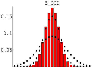
Figure 7: Normalized QCD finite-volume partition function $Z_{\nu}$ as predicted by the Leutwyler-Smilga form (21) (top left) and by the instanton inspired form (24) (top right) for $V\!=\!2\,(1.5\,\mathrm{fm})^{4}$ and $m\!=\!250\,\mathrm{MeV}$. Following the XPT prediction, the topological sectors with $|\nu|\!\geq\!8$ should be populated, but the ILM statistics consideration demands that they are heavily suppressed, since instantons cannot be compressed. The construction (27) assumes that the two high-$|\nu|$ suppression mechanisms do not interfere. The resulting “QCD finite-volume partition function with granularity” is narrower than either one of its predecessors (bottom left), and the topological susceptibility curve derived from it (bottom right) shows all essential features: power-like behaviour for $x\!<\!1$, almost linear behaviour for $x\!>\!1$ and $\Sigma m/N_{\!f}\!<\!\chi_{\infty}$, saturation for $\Sigma m/N_{\!f}\!\geq\!\chi_{\infty}$.

It is now easy see why the topological susceptibility as derived from the finite-volume partition function (21) is, in general, too large. To this end it is useful to consider the distribution of topological charges as predicted by (21) in a box volume typical for full QCD simulations, say $V\!=\!2\,(1.5\,\mathrm{fm})^{4}\!=\!10.125\,\mathrm{fm}^{4}$, at a quark mass of, say, $250\,\mathrm{MeV}$. As one can see from Fig. 7, in this regime the partition function $Z^{\mathrm{XPT}}$ as given in (21) is wider than the partition function $Z^{\mathrm{ILM}}$ as given in (24). In particular, for sufficiently high $|\nu|$ the former indicates a sizable population of that topological sector, whereas the latter is almost zero. This means that the (leading order) chiral prediction neglects the basic fact that instantons form an incompressible fluid [18], i.e. it is impossible to pack such a large number of instantons into the box as the tail of the $Z^{\mathrm{XPT}}$ distribution suggests. This calls for an improvement on $Z^{\mathrm{XPT}}$ which incorporates the unique feature of $Z^{\mathrm{ILM}}$ that instantons occupy a fixed volume. In the absence of an exact analytic solution it is natural to assume that the two suppression mechanisms (captured in (21, 24), respectively) operate independent of each other, i.e. to construct the QCD finite-volume partition function by just multiplying the two asymptotic partition functions

$$Z^{\mathrm{QCD}}_{\nu}=Z^{\mathrm{XPT}}_{\nu}\cdot Z^{\mathrm{ILM}}_{\nu}\;,$$ (27)

as is illustrated in the lower left plot in Fig. 7. As one can see, the resulting distribution is narrower than either one of the asymptotic distributions it was constructed from. This still holds true in the opposite regime of small quark masses where the relationship is reversed (there $Z^{\mathrm{XPT}}$ is narrower than $Z^{\mathrm{ILM}}$ which is quark mass independent). As a result of this the topological susceptibility is smaller than both the XPT-prediction and the ILM-inspired value. This is particularly easy to see in the limit of large box volumes; there either partition function entering the r.h.s. of (27) tends to be gaussian (with variance $\sigma^{2}\!=\!V\Sigma m/N_{\!f}$ and $\sigma^{2}\!=\!V\chi_{\infty}$, respectively), and the multiplication prescription (27) then implies

$$\chi(N_{\!f},m)=1/(N_{\!f}/\Sigma m+1/\chi_{\infty})\;,$$ (28)

which indeed fulfills $\chi(N_{\!f},m)\!\leq\!\min(\Sigma m/N_{\!f},\chi_{\infty})$. Note that (28) is nothing but the member $n\!=\!1$ out of the phenomenological family (6). In addition, two points should be mentioned: First: The nice feature that finite-volume effects in $\chi$ disappear for moderate $(x,V)$ combinations already (say for $x\!\geq\!10,V\!\geq\!10\,\mathrm{fm}^{4}$) has survived. This follows from the construction (27) of the “granular” QCD finite-volume partition function, but one may also verify it by carefully comparing the last graph in Fig. 7 to the dashed (“infinite volume”) curve on the r.h.s. of Fig. 6 – the graph in Fig. 7 was generated for $V\!=\!2\,(1.5\,\mathrm{fm})^{4}\!=\!10.125\,\mathrm{fm}^{4}$, hence reaching $x\!=\!10$ at $m\!\simeq\!62.6\,\mathrm{MeV}$. Second: As a specific finite-volume effect the topological susceptibility curve may show, in a certain (typically narrow) window of (typically small) quark masses, a positive curvature – a feature absent in the infinite-volume limit.

We shall conclude this paragraph with a short reflection on what we have achieved with the “granular” construction (27) of the (true) QCD finite-volume partition function.

On the conceptual level a specific observable, the topological susceptibility $\chi$, has been linked to a more general concept, the QCD finite-volume partition function with granularity. The name reminds one that the expression (21) which resulted from a careful evaluation, at finite $x$, of the QCD partition function in terms of the chiral Lagrangian to order $O(p^{2})$ [8] got modified to account for the “granular structure” of the QCD vacuum, due to instantons. Note that the “granular” partition function depends separately on $V$ and $m$ – not only on the product of them, as (16) and (21) did. The construction is not ad hoc, because the distribution $Z_{\nu}^{\mathrm{QCD}}$ predicts, besides $\chi$, another observable, namely the mass dependence of the sectoral chiral condensate in a finite volume, hence promising an interesting generalization of the results by Damgaard [19]. On the other hand, it is clear that the construction is neither a model nor exact, since subleading effects (where the dynamics of QCD enters) have been neglected; the instanton effect taken into account is pure entropy.

On the practical level, the construction (27) has managed to select, for purely theoretical reasons, out of the phenomenological family (6) the specific member (28) as the one which is, in the limit of large box volumes, most promising. This provides us with an overall fitting curve with just two parameters which is supposed to be reasonable for arbitrary quark mass values. Furthermore, at any given box volume a detailed comparison of the topological susceptibility curve as predicted by (27) to the “infinite volume” form (28) allows one to come up with a quantitative assessment of finite-volume effects on $\chi$. This may prove useful in future simulations of full QCD, since it enables one to choose the box volume just as large as needed in order to keep finite-volume effects tolerable, hence providing some help in the challenging task to allocate computational resources as reasonably as possible. The limiting factor is, of course, that even the demonstrated smallness (within the accuracy of the construction (27)) of finite-volume effects in $\chi$ is no proof that finite-volume effects in other interesting observables would be small.

6 Fits, Cuts and Speculations

We are now ready for a detailed analysis of the available data for the topological susceptibility in 2-flavour QCD.

The most valuable output of the theoretical considerations presented above is a well-motivated functional form against which we may fit the data over the entire range of quark masses. This is particularly useful because, as mentioned in the second section, the bulk of the data is in the transition regime; hence functional forms which are inspired by an expansion appropriate in one asymptotic regime are not guaranteed to yield reliable results for the physical parameters we are interested in.

For large enough box volumes (for details see below) formula (28) will be applicable. It contains two parameters, $\Sigma$ and $\chi_{\infty}$, on which the simulations will disclose some information. Regarding the chiral condensate in the chiral limit, it is important to note that the way it will be determined (via fitting (28) to the lattice data) is logically independent from the usual approach of measuring the condensate at various quark masses via the trace of the Green’s function of the Dirac operator and then extrapolating to zero mass. The procedure to determine $\Sigma$ from the topological susceptibility curve does not require a subtraction or difficult-to-know renormalization constants that arise in more conventional approaches.

	CP-PACS	UKQCD	SESAM	PISA	3-avg	4-avg	all	sel
$2N_{\!f}/(F_{\pi}^{2}r_{0}^{2})$	24.6	46.4	16.4	5.6	29.1	23.3	15.8	24.1
$F_{\pi}$ [MeV]	162.	118.	199.	340.	149.	167.	203.	164.
$\Sigma^{1/3}$ [MeV]	418.	338.	478.	684.	395.	425.	484.	420.
$\chi_{\infty}r_{0}^{4}$	0.063	0.083	0.076	0.035	0.074	0.064	0.054	0.063
$\chi_{\infty}$ [$10^{9}$ MeV4]	1.7	2.2	2.0	0.9	1.9	1.7	1.4	1.7
$\chi_{\infty}^{1/4}$ [MeV]	202.	216.	211.	174.	210.	203.	194.	202.

Table 6: Results of the fits of the data by the individual groups (Fig. 8) or of the combination of all or a selection of them (Fig. 9) to the functional form (28) and of $1/(\chi r_{0}^{4})$ as a function of $1/(M_{\pi}^{2}r_{0}^{2})$ to a straight line, weighting the results 2:1. For both the inverse chiral symmetry breaking parameter (upper part) and the quenched topological susceptibility (lower part) the average over the first 3 or 4 collaborative results is taken in the first line. Successive lines are derived using $r_{0}\!=\!0.49\,\mathrm{fm}$ and, to convert $F_{\pi}$ into $\Sigma$, the values for $M_{\pi},m$ quoted in footnote 5.

Fig. 8 displays the data by CP-PACS (on the $24^{3}\!\times\!48$ lattice only), UKQCD, SESAM and the Pisa group together with individual interpolating curves which represent both reasonable fits of the data to the functional form (28) and of the inverse data versus the inverse argument to a straight line. The respective values for $\Sigma$ and $\chi_{\infty}$ are tabulated in Table 6 (along with further details on how they are determined). A naive average (performed in the top line in either part of the table) yields $\Sigma\!\simeq\!(425\,\mathrm{MeV})^{3}$ and $\chi_{\infty}\!\simeq\!(203\,\mathrm{MeV})^{4}$, respectively, or $\Sigma\!\simeq\!(395\,\mathrm{MeV})^{3}$ and $\chi_{\infty}\!\simeq\!(210\,\mathrm{MeV})^{4}$ if the values suggested by the Pisa group study are not included. A direct fit to the combined data (see Fig. 9) suggests $\Sigma\!\simeq\!(484\,\mathrm{MeV})^{3}$ and $\chi_{\infty}\!\simeq\!(194\,\mathrm{MeV})^{4}$. It seems that the outcome of this combined analysis is influenced, to a huge extent, by the Pisa data – even stronger than the naive average.

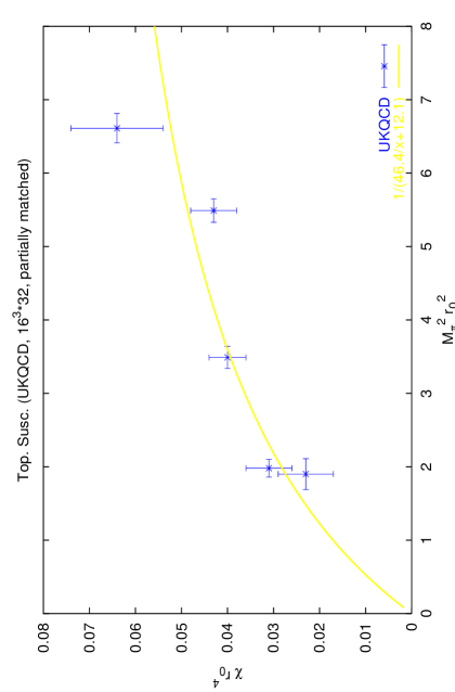
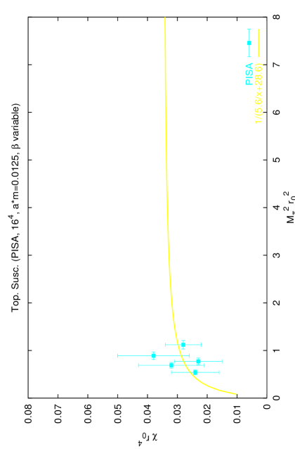
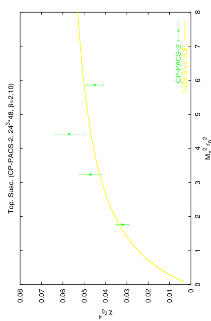
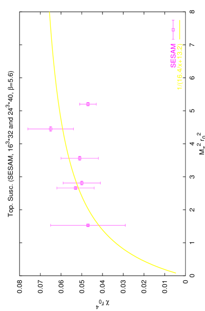
Figure 8: Data generated by CP-PACS, UKQCD, SESAM and the Pisa group for the topological susceptibility versus the quark mass in 2-flavour QCD together with individual fits to the functional form (28). The slopes at zero and the asymptotic values at $m\!\to\!\infty$ determine $\Sigma$ and $\chi_{\infty}$, respectively. Data taken from [3, 4, 5, 6, 9].

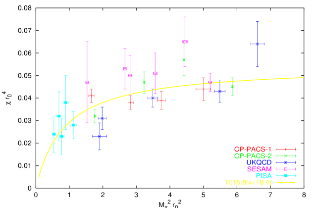
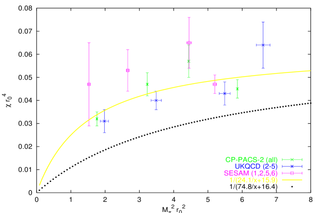
Figure 9: Fitting all data (top) or only those which pass the cuts (29) (bottom) to the functional form (28). Either way $\Sigma$ seems to be much larger than expected, as one can see from comparing the fitted curve to the one anticipated – based on $\Sigma\!=\!(288\,\mathrm{MeV})^{3}$ and the most optimistic value $\chi_{\infty}\!=\!(200\,\mathrm{MeV})^{4}$ – which is included in the second plot. Data taken from [3, 4, 5, 6, 9].

To ensure the quality of the final phenomenological parameters it seems necessary to require the data points to meet certain criteria to be included in the analysis. What we have learned from the previous two sections is that we should not only require $a$ to be reasonably small to keep lattice artefacts under control, but we should also demand the LS-parameter $x$ and the volume $V$ to be reasonably large to keep finite-size effects on $\chi$ moderate and to be able to accommodate a reasonable number of instantons. What I dare proposing, for these reasons, is to apply the following cuts on the data

$$(\mathrm{a})\;\;a\!\leq\!0.15\,\mathrm{fm}\quad,\qquad(\mathrm{b})\;\;x\!\geq\!10\quad,\qquad(\mathrm{c})\;\;V\!\geq\!10\,\mathrm{fm}^{4}\;,$$ (29)

irrespective of the circumstances. From Tables 1-5 one sees that this battery of cuts eliminates the CP-PACS data on the smaller grid and those by the Pisa group. In addition, the UKQCD data set looses its most chiral point, and for the SESAM data only those generated on the larger grid and the two least chiral ones on the smaller grid survive. Table 6 contains, in its last column, the results of a direct analysis of the combined (“selected”) data which have survived the cuts (29). The net outcome almost coincides with the naive average of the results by the individual groups; in the light of the sizable deviations between the results by the various groups (cf. Table 6) I quote

$$\Sigma=(390...430\,\mathrm{MeV})^{3}\quad \mathrm{or} \quad F_{\pi}=145...170\,\mathrm{MeV}$$ (30)

$$\chi_{\infty} = (200...210\,\mathrm{MeV})^{4}$$ (31)

as the current result for $\Sigma$ and $\chi_{\infty}$ when determined via the topological susceptibility curve (and without continuum extrapolation) in 2-flavour QCD.

For the quenched topological susceptibility the result (31) is slightly larger than $\chi_{\infty}$ as determined in previous direct studies in the $SU(3)$ theory [20]. This is not disturbing, since the generally accepted value $\chi_{\infty}\!\simeq\!(190...200\,\mathrm{MeV})^{4}$ is after a continuum extrapolation, whereas the value (31) is gained at finite $a$; hence the difference may – as it is “small” – be attributed to the $O(a^{6})$ term showing up on the r.h.s. of eqn. (12).

For the chiral symmetry breaking parameter the situation seems less pleasing; the result (30) is substantially larger than the generally accepted $F_{\pi}\!\simeq\!93\,\mathrm{MeV},\Sigma\!\simeq\!(288\,\mathrm{MeV})^{3}$, as determined experimentally or via the GOR-relation, respectively (cf. footnote 5). This excess may either be due to lattice artefacts or it may reflect an interesting $N_{\!f}$-dependence of QCD close to the chiral limit. We shall discuss these two possibilities in due course.

Regarding lattice artefacts as a possible reason why (30) exceeds our expectations, little can be said beyond the points already raised in section 4. The issue is not whether lattice artefacts are present – they are, since no continuum extrapolation has been attempted – but rather whether they are numerically under control, i.e. whether the final result (30) is largely influenced by discretization effects or not. The point is that we have just seen that the value (31) for $\chi_{\infty}$ happened to be in rough agreement with our expectations even without a continuum extrapolation, and if lattice artefacts are “small” for the quenched topological susceptibility, it is natural to expect their influence on the other measured quantity, $\Sigma$ (or $F_{\pi}$) to be tolerable too, and this is apparently not the case.

Lattice artefacts have been categorized, in section 4, as (a) scaling violations and (b) chirality violation effects. While these two types of lattice artefacts may, in general, be independent of each other, with Wilson fermions and its descendents (as used in the simulations discussed here) they go together, i.e. they jointly disappear in the continuum-limit and only then. Since in all the data which have passed the cuts (29) smaller quark masses go, in tendency, together with smaller lattice spacings (except for the UKQCD data which are partially matched, cf. Table 3), we would expect the deviations from the dotted curve (which reflects our expectations based on (28) together with $\Sigma\!=\!(288\,\mathrm{MeV})^{3},\chi_{\infty}\!=\!(200\,\mathrm{MeV})^{4}$) to become smaller for low quark masses, if (a) or (b) (or both of them) represent the source of the supposed excess. The bottom part of Fig. 9 (where finite-volume effects are negligible) may contain a hint in this direction: If we suppress the points by the SESAM collaboration (which have huge error bars anyway) the deviation, by absolute standards, of the data from the dotted curve seems to increase towards the r.h.s. (where $a$ is, in tendency, larger). In addition, it looks like there is a slight tendency for the UKQCD data to lie beneath the CP-PACS-2 data. This nicely corresponds with the order of typical lattice spacings as used in these simulations (cf. Tables 2-5), even though unequal efforts have been spent on improving the action. These observations certainly support the view of lattice artefacts as the primary reason why the value (30) for the chiral order parameter exceeds our expectations by roughly a factor 2 (which means a factor $\sqrt{2}$ for $F_{\pi}$), but they are far from conclusive.

The second possibility is that the values (30, 31) are indeed correct, in other words that the problem is not with the lattice determinations of $\Sigma$ (or $F_{\pi}$) and $\chi_{\infty}$, but rather with our expectations – specifically with our knowledge regarding the chiral order parameter. This might come as a surprise, since it is generally believed hat the value $F_{\pi}\!\simeq\!93\,\mathrm{MeV}$ or $\Sigma\!\simeq\!(288\,\mathrm{MeV})^{3}$ is rather well known experimentally or through the GOR-relation, respectively. The point is that the quoted (largely different) values need not necessarily be in conflict with each other, since (30) is determined in $N_{\!f}\!=\!2$ QCD, while the experimental value is in QCD with $N_{\!f}\!=\!3$. The statement is that there might be an $N_{\!f}$-dependence in the topological susceptibility near the chiral limit beyond the one indicated in (5). In other words, there might be an $N_{\!f}$-dependence in the chiral condensate itself which makes $\Sigma_{2}$ as determined in the lattice studies under discussion differ from the experimentally “observed” $\Sigma_{3}$, contrary to the standard belief that $\Sigma_{N_{\!f}}$ is largely independent of $N_{\!f}$.

The idea that $\Sigma$ might depend on $N_{\!f}$ is neither new nor exotic. It is known that QCD has a “conformal window” with restored chiral symmetry if the number $N_{\!f}$ of massless or light flavours is appropriately chosen, i.e. $N_{\!f\,\mathrm{crit}}^{\prime}\!<\!N_{\!f}\!<\!N_{\!f\,\mathrm{crit}}^{\prime\prime}$ [21]. While the upper critical number for this phase is the number of flavours where QCD looses asymptotic freedom, i.e. $N_{\!f\,\mathrm{crit}}^{\prime\prime}\!=\!33/2$ (for $N_{\!c}\!=\!3$) [22], the lower critical number is much under debate. Originally, the Orsay group argued that $N_{\!f\,\mathrm{crit}}^{\prime}$ could be so low (say $N_{\!f\,\mathrm{crit}}^{\prime}\!\simeq\!O(3)$, as opposed to the more standard view $N_{\!f\,\mathrm{crit}}^{\prime}\!\simeq\!O(7)$ [25]) that the chiral condensate in ordinary 3-flavour QCD might be marginal or even vanishing, hence necessitating the extension of the chiral Lagrangian approach [10] to the framework of “generalized chiral perturbation theory” (GXPT) [23]. Meanwhile, they accept that the lower critical bound might be somewhat larger, say $N_{\!f\,\mathrm{crit}}^{\prime}\!=\!O(5)$, but the interesting question remains whether there is any trace of the adjacent “conformal window” for lower $N_{\!f}$-values where QCD is in the confined phase and the chiral symmetry is broken – the latter most likely signaled by the lowest dimensional possible order parameter already, i.e. though $\Sigma\!>\!0$ (distinctively). If in this “ordinary” phase $\Sigma$ would indeed get substantially reduced when $N_{\!f}$ is increased by one unit, such a behaviour could be interpreted as a hint that the real world with $N_{\!f}\!=\!3$ is already “close” to the lower bound $N_{\!f\,\mathrm{crit}}^{\prime}$, as argued by the promoters of GXPT [24]. Hence, if the values quoted in (30) would indeed represent the ultimate truth for $N_{\!f}\!=\!2$ (while still $F_{\pi}\!\simeq\!93\,\mathrm{MeV}$ or $\Sigma\!\simeq\!(288\,\mathrm{MeV})^{3}$ for $N_{\!f}\!=\!3$), this could be taken as an indication that the real world is not too far away from the lower end of the “conformal window”. The important point is, of course, that such a hypothesis is accessible to direct tests on the lattice, and due to those the current body of evidence in favour of a relatively low $N_{\!f\,\mathrm{crit}}^{\prime}$ [26, 27] will either be whiped out or corroborated. As an ironic twist one should note that the value (30) which we supposed as “ultimate” in this scenario and which pushed us into these speculative thoughts is, by its numerical size, anything but marginal.

7 Summary and Outlook

In this paper I have confronted recent lattice data for the topological susceptibility $\chi$ in $N_{\!f}\!=\!2$ QCD as a function of the (dynamical) quark mass with theoretical expectations.

The ultimate goal of these studies is to understand how QCD manages to reduce the prominent $\theta$-dependence of quenched QCD up to the point where it is eliminated, if the chiral limit is taken. Dynamical simulations, by themselves, provide little insight into the mechanism behind this fascinating behaviour; what they can do, however, is to document that the topological susceptibility gets suppressed (and hence the $\theta$-dependence reduced) if the dynamical quark masses are tuned sufficiently small. Pure theoretical thought, on the other hand, may provide interesting bounds and it may yield information about some asymptotic behaviour, but typically the information produced is qualitative, i.e. the relevant constants have to be “borrowed” from elsewhere.

The approach taken here is to combine the lattice data with analytical insight. This is complicated by the fact that the preferred ranges of quark masses are quite different. To be on safe analytical grounds one likes the quarks to be either sufficiently light so that the flavour-singlet axial WT-identity enforces the linear relationship (5) or sufficiently heavy so that the topological susceptibility effectively coincides with its quenched counterpart. The lattice data, on the other hand, happen to be precisely in the intermediate regime which – based on our preliminary knowledge on $\Sigma$ and $\chi_{\infty}$ in QCD – was estimated to be at quark masses of order $88\,\mathrm{MeV}$ in the 2-flavour theory and where the topological susceptibility follows neither one of the two asymptotic patterns.

The key idea on which this article is based is that it is possible to combine the leading physics resources of either regime without invoking specific model assumptions. This is done on the more general level of the finite-volume QCD partition function $Z_{\nu}$ from which the topological susceptibility may be derived. What enters the construction (27) is the assumption that the two mechanisms which suppress configurations with higher $|\nu|$ w.r.t those with lower $|\nu|$ in the small- and the large-mass regime, respectively, operate independently of each other. For small enough quark masses the relevant mechanism is captured in the leading order chiral Lagrangian (which in turn implements the constraint imposed by the axial WT-identity), and the suppression gets manifest upon evaluating the functional integral over the pseudo-Goldstone boson manifold. For large enough quark masses instantons are the relevant degrees of freedom, and an argument is pushed forward that the suppression of higher topological sectors follows from a pure entropy consideration, if instantons are taken incompressible. To the extent that instanton interactions may be neglected and the relevant physics is, on that side, indeed pure entropy, the hypothesis that the two suppression mechanisms are independent is then correct by construction.

On the practical level, the outcome of this analysis is twofold. First, for large enough box volumes the functional form (28) is established as a well-motivated fitting curve, suitable for the entire range of quark masses encountered in present and future studies of QCD with $N_{\!f}\!\geq\!2$ (and $N_{\!f}\!<\!N_{\!f\,\mathrm{crit}}^{\prime}$). It contains only two fitting parameters, and both of them have a direct interpretation in terms of (semi-)phenomenological quantities ($\Sigma$ and $\chi_{\infty}$). Second, the two different choices for the chiral finite-volume partition function $Z_{\nu}^{\mathrm{XPT}}$ (i.e. (16) vs. (21)) entering the construction of $Z_{\nu}^{\mathrm{QCD}}$ allow one to quantitatively assess – within the validity of (27) – the impact of finite-volume effects on the topological susceptibility. The somewhat surprising outcome is that they are smaller than present days statistical uncertainties for relatively small values of the LS-parameter $x$ already, say for $x\!\geq\!10$.

Making use of the functional form (28) the data by CP-PACS, UKQCD, SESAM/TXL and the Pisa group have been analyzed. The results for the asymptotic parameters $\Sigma$ and $\chi_{\infty}$ seem to vary more than what one would have expected from the error bars of the individual data points. While the quenched topological susceptibility $\chi_{\infty}$ is in loose agreement with both the estimate from the Witten-Veneziano relation and previous direct determinations in the quenched theory, the result for the low-energy constant $\Sigma\!=\!-\lim_{m\to 0}\lim_{V\to\infty}\langle\overline{\psi}\psi\rangle$ outstrips the expected value by a factor 2. Here the expectation relies on the GOR-relation and the lattice determination of the non-strange quark mass; would one use a more traditional estimate of $(m_{u}\!+\!m_{d})/2$, the factor by which $\Sigma$ as determined from the topological susceptibility curve exceeds our expectations would be larger. Even restricting the set to contain nothing but “high quality” data (which have passed certain cuts to ensure that effects due to finite lattice spacing and finite box volume should be small) hardly changes the result of the analysis – the $N_{\!f}$-fold asymptotic slope for $N_{\!f}\!=\!2$, $\Sigma_{2}$, stays high.

Two possible reasons for this excess have been discussed. The simple explanation (supported by some inherent features of the data) is that it is due to lattice artefacts. The alternative one (which is mainly discussed because of it conceptual appeal and its potential to initiate dedicated studies) is that $\Sigma_{2}$ is indeed much larger than the GOR-relation suggests, indicating a larger-than-believed $N_{\!f}$-dependence of low-energy QCD. In either case, it seems fair to say that at least in 2-flavour QCD chiral symmetry is predominantly broken through a (distinctively nonzero) chiral condensate [28].

The implication is, of course, that further studies are needed to clarify the situation (cf. [29]). From the analysis one gathers that there are basically three reasonable strategies for going more chiral: to simulate (i) at fixed $\beta$, (ii) at fixed $a$, (iii) at fixed $x$, whereas the possibility (iv) to simulate at fixed $\hat{m}$ seems to yield more questionable results, since in this approach $\beta$ gets so much relaxed that the lattice gets intolerably coarse for the most chiral points. While it is clear that in principle (i.e. if a continuum extrapolation were possible) any of these possibilities would yield the same physical answer, in practice the choice may make a sizable difference, and it is important to keep in mind that the “optimum” choice may not only depend on the regime of quark masses and box volumes one wishes to cover, but also on the actions used. In this respect it is clear that – even if one cannot afford a continuum extrapolation for all the data points constituting the $\chi\!=\!\chi(m)$ curve – a scaling study at least for a single quark mass value might help to get a more quantitative assessment of discretization effects and also to indicate which might be the most promising combination of actions in the gluon and fermion sectors, respectively. If progress turns out to be slow in the $N_{\!f}\!=\!2$ system, studying QCD with $N_{\!f}\!=\!4$ might be an interesting digression – not only because $\Sigma_{4}$ would tell us whether the “conformal window” is close, but mainly for the practical reason that the “transition regime” occurs at higher quark mass values and is therefore cheaper to study. What we are ultimately interested in, however, are the values gained in a more ambitious project, namely the simulation of 2+1-flavour QCD.

Acknowledgements
It is a pleasure to acknowledge interesting and useful E-mail correspondence with Ruedi Burkhalter. In addition, I would like to thank the CP-PACS collaboration for allowing me to show their results for the topological charge distribution on the smaller lattice (Fig. 2).

References

- [1] K. Kanaya et al. [CP-PACS Collaboration], Nucl. Phys. Proc. Suppl. 73, 189 (1999) [hep-lat/9809146].
- [2] E. Witten, Nucl. Phys. B156, 269 (1979). G. Veneziano, Nucl. Phys. B159, 213 (1979).
- [3] A. Ali Khan et al. [CP-PACS Collaboration], Nucl. Phys. Proc. Suppl. 83, 162 (2000) [hep-lat/9909045]. A. Ali Khan et al. [CP-PACS Collaboration], Nucl. Phys. Proc. Suppl. 83, 176 (2000) [hep-lat/9909050].
- [4] A. Hart and M. Teper [UKQCD Collaboration], hep-ph/0004180. A. Hart and M. Teper [UKQCD Collaboration], hep-lat/0009008. A. C. Irving [UKQCD Collaboration], Nucl. Phys. Proc. Suppl. 94, 242 (2001) [hep-lat/0010012].
- [5] G. S. Bali et al., hep-lat/0102002_v3.
- [6] B. Allés, M. D’Elia and A. Di Giacomo, Phys. Lett. B483, 139 (2000) [hep-lat/0004020].
- [7] R. J. Crewther, Phys. Lett. B70, 349 (1977).
- [8] H. Leutwyler and A. Smilga, Phys. Rev. D 46, 5607 (1992).
- [9] S. Aoki, Nucl. Phys. Proc. Suppl. 94, 3 (2001) [hep-lat/0011074].
- [10] For recent reviews of SXPT see e.g: J. Bijnens and U. Meissner, hep-ph/9901381. G. Colangelo, hep-ph/0001256. G. Ecker, hep-ph/0011026. J. Gasser, Nucl. Phys. Proc. Suppl. 86, 257 (2000) [hep-ph/9912548]. B. R. Holstein, hep-ph/0001281. H. Leutwyler, hep-ph/0008124.
- [11] A. Ali Khan et al. [CP-PACS Collaboration], Phys. Rev. Lett. 85, 4674 (2000) [hep-lat/0004010].
- [12] M. Campostrini, A. Di Giacomo and H. Panagopoulos, Phys. Lett. B212, 206 (1988). M. Campostrini, A. Di Giacomo, H. Panagopoulos and E. Vicari, Nucl. Phys. B329, 683 (1990). B. Allés, M. D’Elia, A. Di Giacomo and R. Kirchner, Phys. Rev. D 58, 114506 (1998) [hep-lat/9711026].
- [13] B. Allés, G. Boyd, M. D’Elia and A. Di Giacomo, hep-lat/9610009.
- [14] E. Vicari, Nucl. Phys. B 554, 301 (1999) [hep-lat/9901008].
- [15] This is the outcome of an analysis by G.C. Rossi and M. Testa, announced in [9].
- [16] S. Dürr, Nucl. Phys. B594, 420 (2001) [hep-lat/0008022].
- [17] D. Chen, R. C. Brower, J. W. Negele and E. Shuryak, Nucl. Phys. Proc. Suppl. 73, 512 (1999) [hep-lat/9809091].
- [18] T. Schäfer and E. V. Shuryak, Rev. Mod. Phys. 70, 323 (1998) [hep-ph/9610451].
- [19] P. H. Damgaard, Nucl. Phys. B 556, 327 (1999) [hep-th/9903096].
- [20] J. W. Negele, Nucl. Phys. Proc. Suppl. 73, 92 (1999) [hep-lat/9810053]. M. Teper, Nucl. Phys. Proc. Suppl. 83, 146 (2000) [hep-lat/9909124]. M. Garcia Perez, Nucl. Phys. Proc. Suppl. 94, 27 (2001) [hep-lat/0011026].
- [21] T. Banks and A. Zaks, Nucl. Phys. B 196, 189 (1982).
- [22] D. J. Gross and F. Wilczek, Phys. Rev. Lett. 30, 1343 (1973).
- [23] N. H. Fuchs, H. Sazdjian and J. Stern, Phys. Lett. B 269, 183 (1991). J. Stern, H. Sazdjian and N. H. Fuchs, Phys. Rev. D 47, 3814 (1993) [hep-ph/9301244]. M. Knecht, H. Sazdjian, J. Stern and N. H. Fuchs, Phys. Lett. B 313, 229 (1993) [hep-ph/9305332].
- [24] M. Knecht and J. Stern, in L. Maiani, G. Pancheri and N. Paver (eds.), “The second DAPHNE physics handbook” [hep-ph/9411253].
- [25] Y. Iwasaki, K. Kanaya, S. Kaya, S. Sakai and T. Yoshié, Prog. Theor. Phys. Suppl. 131, 415 (1998) [hep-lat/9804005].
- [26] R. D. Mawhinney, Nucl. Phys. Proc. Suppl. 60A, 306 (1998) [hep-lat/9705031].
- [27] B. Moussallam, Eur. Phys. J. C 14, 111 (2000) [hep-ph/9909292]. S. Descotes and J. Stern, Phys. Rev. D 62, 054011 (2000) [hep-ph/9912234].
- [28] G. Colangelo, J. Gasser and H. Leutwyler, hep-ph/0103063.
- [29] After this work has been completed, two studies have appeared which support the view of discretization effects as the primary reason why (30) exceeds our expectations and provide insight needed to disentangle (a) and (b) as introduced in Sect. 3: A. Hasenfratz, hep-lat/0104015. A. A. Khan et al. [CP-PACS Collaboration], hep-lat/0106010.