Zero temperature string breaking in lattice quantum chromodynamics
Abstract
The separation of a heavy quark and antiquark pair leads to the formation of a tube of flux, or “string”, which should break in the presence of light quark-antiquark pairs. This expected zero-temperature phenomenon has proven elusive in simulations of lattice QCD. We study mixing between the string state and the two-meson decay channel in QCD with two flavors of dynamical sea quarks. We confirm that mixing is weak and find that it decreases at level crossing. While our study does not show direct effects of internal quark loops, our results, combined with unitarity, give clear confirmation of string breaking.
pacs:
11.15.Ha, 12.38.Gc, 12.38.AwI Introduction
In the absence of dynamical sea quarks, the heavy quark-antiquark potential is known quite accurately from numerical simulations of lattice quantum chromodynamics [1]. The potential is traditionally determined from the Wilson-loop observable, which is proportional to at large . At large separation , the potential rises linearly, as expected in a confining theory. In the presence of dynamical sea quarks the potential is expected to level off at large , signaling string breaking. Thus far, no SU(3) simulation at zero temperature with light sea quarks has found clear evidence in the Wilson-loop observable for string breaking [2, 3], even out to fm.
The reason string breaking has not been seen using the traditional Wilson-loop observable is now clear [5, 6, 7]. The Wilson loop can be regarded as a hadron correlator with a source and sink state (F) consisting of a fixed heavy quark-antiquark pair and an associated flux tube. The correct lowest energy contribution to the Wilson-loop correlator at large should be a state “M” consisting of two isolated heavy-light mesons. However, such a state with an extra light dynamical quark pair has poor overlap with the flux-tube state, so it is presumably revealed only after evolution to very large . To hasten the emergence of the true ground state, it is necessary to enlarge the space of sources to include both F and at least one M state.
Drummond demonstrated string breaking in a strong-coupling, hopping parameter expansion with Wilson quarks [7, 8]. A number of numerical studies of theories less computationally demanding than QCD, including nonabelian theories with scalar and adjoint matter fields, found string breaking [9, 10, 11, 12, 13]. One study claims to have found string breaking in the absence of dynamical sea quarks by doing a transfer matrix calculation [14].
In a full SU(3) simulation, until recently, string breaking has only been observed at nonzero temperature (close to, but below the deconfinement crossover) [6], based on the Polyakov loop observable, which evidently has much better overlap with the M state. Some of us reported a preliminary low-statistics result for staggered quarks in 1999 [15], and, last year, Pennanen and Michael announced evidence for string breaking at zero temperature using Wilson-clover quarks and a novel technique for variance reduction in computing the light quark propagator [16]. Duncan, Eichten, and Thacker found hints of a flattening static potential using a truncated determinant algorithm [17].
In this paper we demonstrate string breaking in an SU(3) simulation with two flavors of dynamical sea quarks. Our simulations are done in the staggered fermion scheme on an archive of 198 configurations of dimensions , generated with the conventional one-plaquette Wilson gauge action at and two flavors of conventional dynamical quarks of mass . At this gauge coupling and bare quark mass the lattice spacing is approximately 0.163 fm (based on a measurement of the Sommer parameter[18] extracted from Wilson loops) with a pi to rho mass ratio of 0.358. These parameters were selected to give a relatively light quark, making pair production energetically favorable, and a large lattice volume (about 3.3 fm on a side and 3.9 fm in temporal extent) to allow ample room for string breaking.
II Computational Methodology
Our conventional Wilson loop is computed with APE smearing[19] of the space-like gauge links. Specifically, we used 10 iterations, combining the direct link with a factor (in our case, ) and six staples with factor with SU(3) projection after each iteration. In hamiltonian language the expectation value of this operator is the correlator between an initial and final state , consisting of a static quark-antiquark pair separated by a fat string of color flux. Most of our results are obtained from on-axis Wilson loops with ranging from 1 to 10, but we have two off-axis points at displacement (2,2,0) and (4,4,0) (plus permutations and reflections). Including other off-axis displacements might have been statistically useful[3].
We enlarge the source and sink space by including a meson-antimeson state with an extra light quark located near the static antiquark and an extra light antiquark, near the static quark. To be precise, this state is the tensor product of a static-light meson operator and a static-light antimeson operator. As discussed in Appendix B, staggered flavor considerations make other choices more desirable close to the continuum limit, e.g. the tensor product of creation operators for a flux-tube state and a sigma meson. Our static-light meson construction makes the numerical analysis tractable and is adequate for studying mixing on coarse lattices.
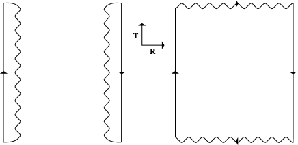
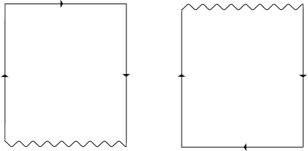
We use an extended source for the light quark in the static-light meson. The heavy quark position, on the other hand, is fixed and used to define the separation . Specifically, the gauge-invariant source wavefunction at a site has support only on the site itself and on the second on-axis neighbors in all six spatial directions, connected to the central site by a product of the APE smeared links along the paths. Rather arbitrarily, the central site is given weight 2 while the satellite sites have weight 1. Thus we also compute the additional correlation matrix elements , and . They are diagramed in Figs. II and II.
For the light quarks in the static-light mesons we use the same parameters as for the dynamical sea quarks. To reduce variance we generated “all-to-all” propagators for the light quark, using a Gaussian random source method [4]. (See Appendix A). Results reported here are based on 128 such sources per gauge configuration, which gave satisfactory statistics for our lattice volume. With this number of sources the variance due to fluctuations in random source was comparable to that due to fluctuations in the ensemble of gauge configurations.
We analyze our correlators using an extension of the transfer matrix formalism of Sharatchandra, Thun, and Weisz[20] for staggered fermions, described in Appendix B. With our choice of local meson operators, discrete lattice symmetries, also discussed in Appendix B, require that all products of gauge links in the observables be assigned phases consistent with being viewed as the paths of heavy staggered fermions. For example, for the Wilson-loop operator, a hopping parameter expansion around an on-axis rectangular path gives, in addition to the conventional Wilson-loop gauge-link product, a net phase factor , independent of the staggered fermion Dirac phase conventions. (Included is a factor for a single closed fermion loop.) This phase then controls the sign of the transfer matrix eigenvalue associated with the flux tube state. We use a similar construction to get the phases for the nonclosed gauge-link products in the diagrams of Figures II and II. In all cases the Dirac phase convention for the gauge-link products must be consistent with that of the light quark. A consequence of this construction is that the correlation matrix elements involving off-axis gauge-link products must vanish when summed over symmetry-equivalent paths for net displacements that have more than one odd Cartesian component.
III Staggered Fermion Pair Production
A Transfer matrix eigenvalues
The heavy quark potential is defined as the ground state energy of the QCD hamiltonian with a static quark and antiquark separated by distance . Operationally, we extract the ground state energy by fitting the time dependence of the correlation matrix elements in the same manner as one obtains hadron masses. Fundamentally, the potential is determined by the eigenvalues of the transfer matrix. To justify our fitting ansatz, therefore, we start from an analysis of the transfer matrix in the staggered fermion scheme.
Transforming to temporal axial gauge and making a suitable choice of fermion phases, Sharatchandra, Thun, and Weisz showed that the staggered fermion transfer matrix is hermitian but not positive [20]. Then, it is convenient to use the eigenvectors of the transfer matrix as a basis for representing the correlation matrix. In terms of the (possibly negative) eigenvalues of the transfer matrix, our correlation matrix can therefore be written in spectral decomposition as
| (1) |
where refer to the flux tube or meson-meson states. The power is natural, as we show in Appendix B. This result forms the basis for our fitting ansatz. To apply this decomposition to our results, it is essential, as we have done, that we treat the heavy quark lines as static staggered quarks, with all fermion phases included, and that source and sink operators are equivalent.
B Static light propagator
We first examine the single static-light meson correlator, shown in Fig. III B. We find good fits to two spectral components, one with no phase oscillation in , corresponding to a -wave light quark and a positive transfer-matrix eigenvalue, and the other, higher in energy, and with oscillating phase in , corresponding to a -wave light quark and a negative transfer-matrix eigenvalue. Fitting to a single nonoscillating exponential plus a single oscillating exponential over the range gives energies (defined as usual as ) and with . The -wave amplitude is suppressed by a factor of about 0.5 relative to the -wave amplitude.

C Fitting form for the correlation matrix
Since we expect to find two static-light mesons at large in our correlator, we look for a positive eigenvalue “SS” spectral component corresponding to two -wave mesons and a negative eigenvalue SP component corresponding to an -wave and -wave meson. For most of our analysis we omit the PP component, a choice that we justify as follows: Squaring the static light propagator suggests that the PP channel would contribute a second nonoscillating spectral component at a higher energy (about 0.5 in lattice units) than SS and with a smaller amplitude (about 0.2). We present results, however, that include a excited state component inspired by the PP contribution. The SS and SP components would be expected to have a smooth dependence on for large . To these two spectral components we add a third, corresponding to a conventional Wilson-loop contribution at short distance . With the staggered fermion phases included, the net Wilson-loop phase factor produces a transfer matrix eigenvalue with a phase that oscillates with .
Our proposed fitting ansatz is thus Eq (1) with and with the explicit SS, SP, and flux-tube eigenvalues (respectively)
| (2) | |||||
| (3) | |||||
| (4) |
Other components can be readily included. With our choice of sources and sinks the correlation matrix is found to be real, so we may take real factors. An ambiguity permits changing the sign simultaneously in and , which we resolve arbitrarily by requiring to be positive. At large we expect to approach and to approach and at small we expect to correspond roughly to a Coulomb plus linear heavy quark potential. At intermediate we expect mixing among these states. Avoided level crossing may occur at even between intermediate states 2 and 3 and at odd between intermediate states 1 and 3.
IV Results
A Potential
With the factorization inherent in our ansatz (1) and the choice , we are fitting three correlators with nine parameters. Our fitting range in varies over the data set as shown in Table I with typically 10 or more degrees of freedom. The goodness of fit supports our ansatz.
Our selection of fit ranges compromised between the need to get acceptable fits and our intention to vary the end points and smoothly as a function of . At low the (flux-tube-type) correlator has quite small errors, whereas at larger , errors increase, especially at higher . Thus for small we can set a higher in the correlator to improve chi square without loss of information. At larger there seems to be little improvement in goodness of fit in setting a high , and the large statistical errors at high give no advantage to setting a higher .
To give an impression of the quality of the fits, we plot the absolute value of the correlation matrix elements vs for two values of in Figs. IV A and IV A. Also plotted are the absolute values of the fitting functions. The errors on the observed and correlators also give an indication of the signal obtainable with the random source method.


Results at are a good representative of the small correlators and the degree to which the fit results are affected by the choice of end points. Fitting the three correlators , , and over the ranges , , and , respectively, gave , , and with . Changing the fit ranges to , , and increased to 23.6/15 and gave , , and .
To see the effect upon the mixing analysis of including other states, we experimented with adding an excited state modeled after the two-meson PP spectral component, which contributes in the same way as the SS component. The fourth spectral component is denoted . Doing so increases the parameter count to 12. To assure stability of the fits, we fixed the two-meson energies and , leaving 10 free parameters. We found acceptable fits. The unconstrained energies and agreed within errors with results from the three-spectral-component ansatz. For example at over fit ranges , , we find with and .
Our fit results for the three-spectral-component ansatz are listed in Tables I and II and plotted in Fig. IV A. For small distances the flux tube energy is smallest and the flux tube state dominates the large behavior of the correlation matrix, while at large distances the two-meson energies and are smaller and the two-meson states dominate the correlation matrix at large . With our choice of light quark mass the first level crossing occurs at , or 0.98 fm. The string is broken. It is interesting that the energies and are very nearly equal to their asymptotic values throughout. Thus we see no spectral evidence of a meson-meson interaction at the level of our statistics.
It is clear from these results that mixing between the flux-tube and two-meson channels is weak. There is no evident rounding of the potentials normally associated with avoided level crossing. At higher order in mixing we would expect to require two-meson spectral components in the flux tube correlator. They should appear as a result of the breaking and rejoining of the string. However, the amplitudes for both terms in this correlator are small enough that, if it weren’t for the enforcement of a common spectrum and factorization in our fit ansatz, they might have been missed. The converse presence of the string term in the diagonal two-meson correlator can be accounted for by the “box” diagram in the quark correlator that resembles a Wilson loop.
As a check of mixing between the flux-tube level and the two-meson levels, we examined the transition amplitude to see if, by itself, it contained both types of spectral components [21]. To do so we carried out a separate three-exponential fit to the transition amplitude alone, fixing the energies of the , , and flux-tube spectral components to the values found in the multichannel channel analysis, but adjusting their amplitudes for a best fit. For , where the spectral components are clearly nondegenerate, we found that the amplitudes for the and flux-tube components were both nonzero at the three to five-sigma level. Thus our results, combined with unitarity, confirm mixing and imply string breaking.
We have required that the valence and sea quarks match, thus assuring that the correlation matrix is a power of the transfer matrix. However, if mixing effects are very weak, had we chosen, instead, to omit the dynamical sea quarks altogether, it would very likely be difficult to detect the consequent inconsistencies. We analyze mixing further in the following subsection.

B Modeling the mixing
Drummond, Pennanen and Michael analyze their results in terms of a transfer matrix model that mixes the two-meson and flux-tube states [7, 16]. Our approach differs slightly, because our multi-exponential fit carries more information and because our multi-channel contributions complicate the analysis. A perturbative model of string breaking starts with a zeroth order pure flux-tube state () and a pure two-meson state, consisting of either a pair of unperturbed -wave mesons () or unperturbed - and -wave mesons (). (By extension, we could include the channel.) At a given the lattice mixing between the states can be described by a transfer matrix on the unperturbed basis
| (5) |
that evolves a state across a Euclidean time slice. The rows and columns are arranged in the order , , and . We assume a small value for the mixing between and and between and . Although the and states may mix, for simplicity, we have ignored this effect. The diagonal elements correspond to our conventions for our fit ansatz (3). The correlation matrix connecting our flux-tube and two-meson source and sink states at a given is
| (6) |
where is the unperturbed matrix used in our fit ansatz. The diagonal elements of and the potentials are unperturbed at first order in and . The off-diagonal correlator to first order is
| (7) |
where
| (8) | |||||
| (9) | |||||
| (10) |
To first order in the mixing parameters, the factors are unperturbed, and we may equate to obtain three constraints for the two mixing parameters and . The third constraint is a sum rule. To apply the model we chose to impose the sum rule as an a posteriori constraint on the parameters of the fit for each :
| (11) |
and use the first two conditions to determine the mixing parameters:
| (12) | |||||
| (13) |
This was done by linearizing the sum rule in the vicinity of the minimum of the unconstrained :
| (14) |
It is straightforward to determine the attendant increase in , the shift in parameters, and the decrease in errors. Since this procedure assumes the sum rule can be linearized, it is valid only to the extent that the increase in is small.
Table III lists results. Shown are the values of the coefficient ratio
| (15) |
before and after imposing the linearized sum rule constraint as well as the shifts in and the values of and obtained after imposing the constraint. The ratio should be one if the sum rule is satisfied. We see that the increase in is smallest for , but it is otherwise unacceptably large. Thus the mixing model suits our three-exponential ansatz only for larger . The agreement improves considerably when we include the two-meson PP spectral component, as discussed above, and fix the two-meson energies and , leaving 10 free parameters. Although we include the fourth component in the fit, we still consider only a three-state mixing model. (In effect, we have set mixing to the fourth level to zero.) Results are shown in Table IV. Now the mixing model seems plausible for .
The mixing model makes separate predictions for the connected and disconnected meson-to-meson correlators, which provides an additional constraint on the mixing parameters. As a test of the systematic error arising from model assumptions, we have tried refitting all of our data to a purely four-component mixing model, with separate disconnected and connected correlators. While the resulting mixing coefficients repeat the trends of Tables III and IV, the values differ as much from those of the tables as the two tables do from each other.

If we now take the mixing model at face value, it is interesting to consider how the strength of mixing varies with . In Fig. IV B we see a significant decrease in both and with increasing , which is to be expected partly from (13) as the eigenvalues cross. There is also a pronounced difference in mixing strengths at even and odd , suggesting a suppression of mixing between unperturbed oscillating and nonoscillating levels. Obviously, given the coarseness of our lattice, the comparison with a model Hamiltonian must be done judiciously. However, even these first, crude QCD results should help constrain the phenomenological analysis of quarkonium decay [22].
V Conclusions
We have studied string breaking in the heavy quark interaction at zero temperature in QCD. Our calculation used two flavors of light staggered quarks and gauge configurations generated in the presence of the same quarks. We extended the analysis of the spectrum of the transfer matrix in the staggered fermion formalism to treat our nonlocal sources. By adding explicit two-meson states to the conventional flux-tube state, we obtain the expected result that the two-meson state is energetically favored at large distance. Our two-channel correlators fit a model with three factorizing spectral components and a partially constrained, extended model with four spectral components. Our results are also consistent with a simple three- and four-state model with weak mixing. The mixing coefficients in the mixing model matrix appear to decrease at the level crossing points. Our principal finding is that mixing between the flux-tube and two-meson channels is indeed weak. Thus we see why string breaking has been missed in the flux-tube channel by itself. While our matching of dynamical and valence quarks is designed to satisfy unitarity, with our statistics we have not found compelling evidence for quark loop effects. Doubtless, our results could have just as well been reproduced in a quenched simulation, where inconsistencies with unitarity would appear only at higher order in the mixing matrix elements. However, we also find that the transition correlator by itself connecting flux-tube and two-meson channels is nonzero for all and shows both string-like and two-meson-like spectral components, at least for . Thus, our results, combined with unitarity, require string breaking. It is recommended that future staggered fermion studies closer to the continuum take care to restrict the two-meson wave function to the light-flavor singlet channel.
Acknowledgements.
Gauge configurations were generated on the Indiana University Paragon. Calculations were carried out on the IBM SP at SDSC and the IBM SP and Linux cluster at the University of Utah Center for High Performance Computations. This work was supported by the U.S. Department of Energy under grants DEFG0291ER40661, DEFG0291ER40628, DEFG0395ER40894, DEFG0395ER40906, DEFG0596ER40979, and the National Science Foundation under grants PHY9970701 and PHY9722022.A Random Source Estimators Applied to String Breaking
We use random source methods to calculate the all-to-all quark propagators in this study. Here we outline the method as applied to string breaking. We begin with the conventional light quark propagator
| (A1) |
which satisfies the equation
| (A2) |
Summation over repeated indices is implied unless noted otherwise. denotes the usual staggered lattice Dirac operator.
The static (infinitely heavy) quark propagator can be found from an expansion to leading order in . The result depends on whether propagation is forward or backward in time. For , omitting the heavy quark mass factors,
| (A3) |
where
| (A4) |
and the are staggered fermion phase factors. For
| (A5) |
where
| (A6) |
We will be interested in static-light mesons, which we construct from the Grassman fields as
| (A7) | |||||
| (A8) |
The wave function is hermitian, , and depends via gauge fields on . We use
| (A9) |
The space-like gauge-link matrices can be taken as (APE) smeared gauge fields. Thus the tilde here represents both smearing and the inclusion of the fermion hopping phases. On the other hand the time-like gauge-link matrices are not smeared.
For the static-light meson correlation function with source at the origin we obtain
| (A10) | |||||
| (A11) |
where
| (A12) |
is the product of link matrices and hopping phase factors from to . In the last line we introduced Gaussian random numbers, , to compute the trace. Multiplied by they form the source for the light quark inversion and are then used again in the computation of the static-light meson correlation function as seen in eq. (A11). Introducing the smeared, random source propagator
| (A13) |
we can write the static-light meson correlation function as
| (A14) |
In numerical practice this result is computed for a source at any lattice location and averaged over the space-time volume.
For the computation of the heavy quark potential and the investigation of string breaking we will need a heavy quark-antiquark “string state”
| (A15) |
where is a superposition of products of (APE smeared) gauge fields in time slice starting at and ending at .
We are then interested in the diagonal correlator between a string state at time and one at time we consider the connected part only
| (A16) |
with smeared space-like gauge field product segments in the time-like Wilson loop . Except for the fermion hopping phases, which give a net factor independent of staggered fermion phase convention, this is the correlation function usually considered for the computation of the heavy quark potential. As usual, in practice this quantity is averaged over all choices of lattice origins and on-axis displacements . We also computed it for two off-axis displacements, namely and . For off-axis displacements is constructed from a symmetric set of space-like paths joining the endpoints.
We are also interested in the off-diagonal correlator between the string state and the two-meson state
| (A17) |
| (A18) | |||||
| (A19) | |||||
| (A20) |
The with four coordinate arguments stands for the product of time-like and (APE smeared) space-like gauge fields that make up the part of a time-like Wilson loop without the spatial segment at time . Again, this correlator is computed with the Gaussian random source method, in a manner similar to the static-light meson correlation function (A11). The other off-diagonal correlator, , is the hermitian conjugate of (A18). This quantity is averaged over the same choices of origin and displacement as the Wilson loop.
Finally, we need the two-meson correlator
| (A21) | |||||
| (A22) | |||||
| (A23) | |||||
| (A24) | |||||
| (A25) |
We compute the two terms in eq. (A23) again with the Gaussian random source method using two independent Gaussian sources, and , one for each of the two light quark propagators:
| (A26) | |||||
| (A27) | |||||
| (A28) |
Again, this quantity is averaged over the same choices of origin and displacement as the Wilson loop. It is important to note from our expressions for the correlators that all can be computed using methods for random sources.
B Transfer Matrix Applied to String Breaking
We review the Sharatchandra-Thun-Weisz (STW) Fock-space formulation of the staggered fermion partition function with specific application to the operators used in our string breaking study [20].
1 Introduction
The fermion action is given by
| (B1) |
where the spatial part of the action is
| (B2) |
With the STW phase convention
| (B3) | |||||
| (B4) |
With this choice the phases have no dependence. The imaginary time variable ranges over , and the antiperiodic boundary condition requires .
The partition function is given by
| (B5) |
where and denote the full set and . We would like to convert the Grassmann integral into a Fock-space operator trace. To this end STW first eliminate the KS phase in the time direction altogether, by changing variables to . The spatial action becomes
| (B6) |
where
| (B7) |
Then STW introduce a dummy set of Grassmann variables and . The action is then
| (B8) |
where we have suppressed the sum over spatial coordinate . The partition function now includes integration over the dummy variables with a delta-function constraint:
| (B9) |
Here the delta function implies a product over delta functions on each lattice site. The Grassmann delta function is simply
| (B10) |
We introduce a Fock space by associating creation and annihilation operators with each Grassmann variable. The corresponding Fock space operators are denoted by a hat. It is convenient to introduce Grassmann coherent states [23]:
| (B11) | |||||
| (B12) |
The coherent states satisfy completeness and trace relations:
| (B13) | |||||
| (B14) |
With these identities we can reorganize the factors in in the form
| (B15) | |||
| (B16) |
where denotes operator normal ordering. Using the completeness and trace identities and the antiperiodic boundary condition, we can then write the partition function in terms of a transfer matrix operator:
| (B17) |
where
| (B18) |
This is a manifestly Hermitian, but not positive definite, transfer matrix.
2 Quantum mechanics
To see how this transfer matrix works, as a warmup exercise, suppose there is only one spatial site (quantum mechanics). The transfer matrix is then
| (B19) |
It has eigenstates ()
| (B20) |
with eigenvalues . Thus the ground state is . The “degenerate” and states are interpreted as single particle and single antiparticle states, and the state , as a state with a particle and antiparticle pair. The partition function is ( even)
| (B21) |
Next we consider the propagator for a single massive fermion, created at time slice 0 and propagating to time slice .
| (B22) |
Converting to the Fock space basis as we did with the partition function leads to
| (B23) |
This example shows that a power is natural. If we assume that is large, so only the ground state contributes to the traces, we have ()
| (B24) |
with interpreted as the energy of the propagating state. For large mass the correlator is approximately .
The antiparticle propagator (with instead) is also easily computed with the result
| (B25) |
Next, we introduce a second heavy flavor of mass (), denoted by . We consider the propagation of a heavy-light meson. For simplicity we use an interpolating operator with a local (point) wave function. In this case the Grassmann integration involves the combination . Following the same steps as before leads to
| (B26) |
3 String-breaking operators
Here we construct the operators required for our string-breaking study. Two interpolating operators, and , are used, one that creates a static quark-antiquark pair with a connecting flux tube and another that creates a pair of static-light mesons. A simple way to construct the flux tube operator is to introduce a new heavy flavor of mass . Our conventions for the on-axis (direction ) string-creation operator can be obtained from the Grassmann product after integrating out the new flavor in the static limit . The result is a heavy quark-antiquark creation operator connected by the static quark propagator. In the Grassmann basis it is
| (B27) |
Our corresponding annihilation operator is similarly generated from the product , yielding
| (B28) |
(With all of our static quark propagators, it is convenient to introduce a separate, heavy flavor for each straight-line segment.) The meson-antimeson creation and annihilation operators are simply
| (B29) | |||||
| (B30) |
We are interested in the two-channel correlators in the static limit with the heavy quarks fixed at and :
| (B31) |
where . The conversion to Fock space proceeds as before. With the Fock space operators are
| (B32) | |||||
| (B33) | |||||
| (B34) | |||||
| (B35) |
We recall that is independent of , and , so the dagger indeed denotes the Fock space hermitian conjugate. The desired correlators are then
| (B36) |
An eigenstate of the transfer matrix with eigenvalue contributes
| (B37) |
where
| (B38) |
This result is the basis for Eq. (1).
4 Staggered spin and flavor considerations
The external states in our analysis are built from two operators: one that creates a static quark-antiquark pair at separation and one that creates a pair of static quark-light quark mesons at separation . Both the static quark and light quark carry four continuum flavors. One may ask, in the continuum limit, what spin, parity, and flavor combinations occur?
a Flavors and spins of the static-light meson
Golterman and Smit [25] give an analysis of the flavor content of staggered quark-antiquark mesons. Our static-light meson wavefunction has a local component (zero displacement) and a component with displacement 2 along any axis. An even displacement does not change the light-quark flavor and spin wavefunction, so for simplicity we analyze only the local component,
| (B39) |
where the c.m. offset ranges over the eight sites in a unit cube.
The more familiar flavor-spin content is displayed in the notation of Kluberg-Stern et al. [24]:
| (B40) |
where a sum over four flavor and four spin indices is assumed, and
| (B41) |
A similar expression holds for the heavy quark operator . We have ignored the gauge connection in these expressions. The coefficients give the flavor-spin wavefunction of a quark created at site .
The zero-three-momentum projection of the local static-light operator is given by
| (B42) |
All eight operators, corresponding to the eight values of , belong to Golterman’s class 0. Because the static quark must propagate in place, the correlation matrix for these eight states is diagonal in and independent of . Apart from a volume factor, it is exactly the static-light correlator we have computed. Linear combinations of these operators with coefficients differing only by signs yield operators belonging to the rest-frame symmetry group of the discrete transfer matrix. For example, the operator belonging to the one-dimensional representation in the Golterman-Smit notation is given by
| (B43) |
In the Kluberg-Stern et al. basis this operator is written as
| (B44) |
where the first gamma factor in the tensor product operates on the spin basis and the second, the flavor basis, and the sign is plus for even and minus for odd.
This operator generates both a pion-like and sigma-like state in the continuum, in which, respectively, the light quark is found in an or orbital around the static quark. Similar linear combinations yield eight operators, altogether belonging to the irreps , , , and , each interpolating one of eight -wave channels: two pion-like (-mesons) and two rho-like (-mesons). Each of these is paired with one of eight -wave channels: two sigma-like and two pseudovector-like, respectively. All -wave states are degenerate, as are all -wave states. A fixed offset corresponds to a distinct linear combination of these degenerate states. Alternatively, we may say that a fixed offset corresponds to the pairing of a single flavor-spin species of light quark and heavy quark.
Thus our two-meson operator interpolates all combinations of and and their -wave counterparts. Our procedure for computing correlators sums over all cubic rotations of at fixed , so is consistent with zero total angular momentum for the two-meson and flux-tube states. Transitions of the type are accompanied by a change in orbital angular momentum.
Static-light mesons in the Golterman classes 1, 2, and 3 are similarly degenerate within each class with multiplicities 24, 24, and 8, respectively. One would expect in analogy with the light mesons that on a coarse lattice the energies of the class nonzero static-light mesons are higher than that of class 0. In the continuum limit all 64 become degenerate because of flavor and heavy quark symmetry. A multiplicity factor of 16 comes from separate heavy-flavor and light-flavor symmetry and a multiplicty factor of for degenerate singlet and triplet spin combinations.
b Flavors and spins of the static-static meson
The flux-tube operator is designed so that it belongs to the same representation of the symmetry group of the transfer matrix as the meson-antimeson operator, thus permitting mixing of the states they create. The zero momentum projection of the meson-antimeson operator at any separation is in Golterman class 0. At the flux-tube operator creating a static quark-antiquark pair is trivially one of eight Golterman class 0 operators. For it to remain in this class as the quarks separate, one must include the hopping phases with the gauge-link operators that excite the electric flux accompanying the creation of the static pair (A4). A simple way to see this is to consider that the operator class is a symmetry of the transfer matrix, so acting upon the zero separation state with the heavy-quark hopping matrix, which incorporates the phases, preserves the operator class. The eight operators consist of two pion-like and six rho-like operators. More specifically, the static-quark-antiquark operator at all is a linear combination of the two local (heavy quark) pseudoscalars and and the six local vector mesons and . In the -quark system, these states would be classified as the and the .
In free (static) propagation the even parity -wave partners of both are trivially absent in the static limit. On the other hand, in the presence of dynamical staggered quarks and in the strong-coupling limit, we see no reason that dynamical quark loops could not generate an anomalous, opposite-parity partner in the Wilson loop correlator at second order in the mixing coefficients. Thus, the appearance of both oscillating and nonoscillating components in the Wilson loop would be a signal of string-breaking at strong coupling. In the continuum limit the anomalous components should vanish, in keeping with the expectation that lattice staggered and nonstaggered fermion actions have identical limits. On our moderately coarse lattices, in the transition correlator connecting the flux-tube and meson-antimeson channels, the signal appears in leading order, but from our mixing analysis, we find that the anomalous parity component is smaller.
c Light flavor artifacts in the meson-meson correlator
The peculiarities of staggered flavor symmetry require paying special attention to light quark flavor counting. Two issues confront us. First, in our meson-antimeson channel, in the continuum limit the light quarks can combine as a flavor singlet or flavor non-singlet with, in principle, distinct energies. Since the flux-tube state is necessarily a light-flavor singlet, only the singlet components mix, leaving the nonsinglet as a potential additional spectral component. Second, the gauge configurations were generated in the presence of flavors, through the usual device of taking the square root of the intrinsically four-flavor fermion determinant. However, the light quarks in our source and sink carry four flavors. A mismatch between the number of valence and sea quarks gives rise to additional spectral components in the disconnected meson-to-meson correlator.
To count flavors, we construct a toy model similar to the mixing model of subsection IV B. However, for present purposes we ignore negative transfer matrix eigenvalues and deal directly with the Laplace transform of the correlators. Further, it is sufficient to concentrate on the meson-meson correlator .
We begin with the disconnected meson-meson correlator at a fixed separation . As we have noted above, the static-light mesons are created in Golterman class 0. In the absence of glueball exchange between the meson and antimeson, they remain in class 0. Glueball exchange can excite class levels in pairs. Such an effect is presumably short range, because the glueball mass is of order one GeV. Thus, on a coarse lattice we expect four distinct energy levels, and the Laplace transform of the correlator has the form
| (B45) |
At least for larger than a few tenths of a fermi we expect the lowest level to have the largest overlap with the source and sink so that for . So we simplify our model, writing
| (B46) |
where the remaining terms are higher energy and weakly coupled, except, possibly, at small .
In the continuum limit flavor symmetry requires only two energy levels, depending on whether the light quarks form a flavor singlet or nonsinglet. Thus we use to denote the singlet and , the nonsinglet. Since our source/sink operator generates a single flavor-spin species of light quark and light antiquark, for four light flavors the relative weight of singlet to nonsinglet is , and we get
| (B47) |
Next, we consider the connected correlator . We treat light quark pair annihilation and creation as a weak process with amplitude and analyze this correlator as a perturbation series in . Thus the leading term in the connected diagram has the form
| (B48) |
where is the energy of the flux-tube state. The amplitude gives the weight for annihilation or creation of a single light quark/antiquark flavor. Here is the sequence of events: The source state couples to the lowest level, which propagates with energy . It then annihilates with amplitude to produce the flux-tube state, propagating with energy . Pair creation leads back to the lowest level, which propagates with energy before coupling to the sink.
The next higher order contribution to comes from a quark-loop insertion. The sequence of events is the same as in the leading-order contribution, except that an extra pair creation and annihilation process occurs in the flux-tube state. Pair creation on a coarse lattice leads to any of the four levels at the same order in . In the continuum limit and large these levels are degenerate, and would each count with weight , the factor arising from the fermion determinant. For simplicity, to model the full effect of the internal quark loop, we assign it a weight with in the continuum and represent only the lowest level . Thus we have
| (B49) |
Continuing with these simplifications to all orders, we may sum the perturbation series to obtain , where
| (B50) |
The ellipsis represents contributions to the disconnected diagram from light-flavor nonsinglet terms.
This toy flavor-counting model shows the desired shifted pole at , but additional, complicating spectral components at , , and the light-flavor nonsinglet level(s). These additional components are an artifact of our choice of source and sink. While, in principle, one may carry through the spectral analysis of the correlators, remembering to include the artifacts, the analysis would be unnecessarily complicated. For the present numerical study, weak mixing and strong flavor symmetry breaking on our coarse lattice render the extra spectral components harmless. First, strong coupling breaks flavor symmetry and lifts the levels above , making it less likely to confuse them with . Second, because of weak mixing, we are unable to detect the internal quark loop directly. Thus we measure the mixing parameter , but do not see .
Closer to the continuum, it is desirable to replace the meson-meson interpolating operator with a better one, building in an explicit projection of the light-quark flavor singlet. An example is a state formed from the tensor product of a meson and a static quark-antiquark flux-tube. Clearly, such a projection eliminates the nonsinglet contribution. But to eliminate the other artifacts also requires in the toy model, which is not automatic when there are two sea quark flavors but four source and sink flavors. The remaining artifacts are eliminated by adjusting the weight of the disconnected diagram, relative to the connected diagram. To be precise, once a projection to an SU(4) flavor singlet has been done in the state , the proper weighting is .
REFERENCES
- [1] G. Bali and K. Schilling, Phys. Rev. D 46, 2636 (1992); 47, 661 (1993); S.P. Booth et al. (UKQCD Coll.), Phys. Lett. B 294, 385 (1992); Y. Iwasaki et al., Phys. Rev. D 56, 151 (1997); B. Beinlich et al., Eur. Phys. J. C 6, 133 (1999), [hep-lat/9707023]; R.G. Edwards, U.M. Heller and T.R. Klassen, Nucl. Phys. B517, 377 (1998).
- [2] K.D. Born et al., Phys. Lett. B 329, 325 (1994); U.M. Heller et al., Phys. Lett. B 335, 71 (1994); U. Glässner et al. (SESAM Coll.), Phys. Lett. B 383, 98 (1998); C. Bernard et al. (MILC Coll.), Phys. Rev. D 56, 5584 (1997); S. Aoki et al. (CP-PACS Coll.), Nucl. Phys. B (Proc. Suppl.) 63, 221 (1998). S. Tamhankar and S. Gottlieb, Nucl. Phys. B (Proc. Suppl.) 83-84, 212 (2000). M. Talevi et al. (UKQCD Coll.), Nucl. Phys. B (Proc. Suppl.) 63, 227 (1998).
- [3] B. Bolder et al., Phys. Rev. D 63, 074504 (2001) [hep-lat/0005018].
- [4] It has been argued that Z(2) noise methods are superior. S. Dong and K. Liu, Phys. Lett. B 328, 130 (1994)
- [5] C. Michael, Nucl. Phys. B (Proc. Suppl.) 26 (1992) 417.
- [6] C. DeTar, O. Kaczmarek, F. Karsch and E. Laermann, Phys. Rev. D 59, 031501 (1999).
- [7] I. T. Drummond, Nucl. Phys. B (Proc. Suppl.) 73, 596 (1999).
- [8] I. T. Drummond, Phys. Lett. B 434, 92 (1998).
- [9] F. Knechtli and R. Sommer [ALPHA collaboration], Phys. Lett. B 440, 345 (1998) [hep-lat 9807022]; Nucl. Phys. B 590, 309 (2000) [hep-lat/0005021].
- [10] P. W. Stephenson, Nucl. Phys. B550, 427 (1999).
- [11] P. de Forcrand and O. Philipsen, Phys. Lett. B475, 280 (2000). [hep-lat/9912050].
- [12] O. Philipsen and H. Wittig, Phys. Rev. Lett. 81, 4056 (1998).
- [13] H. Trottier, Phys. Rev. D 60, 034506 (1999)
- [14] C. Stewart and R. Koniuk, Phys. Rev. D 59, 114503 (1999).
- [15] C. DeTar, U. Heller, and P. Lacock, Nucl. Phys. B (Proc. Suppl.) 83, 310 (2000).
- [16] P. Pennanen and C. Michael [UKQCD Collaboration], “String breaking in zero-temperature lattice QCD,” [hep-lat/0001015].
- [17] A. Duncan, E. Eichten, and H. Thacker, “String Breaking in Four Dimensional Lattice QCD”, [hep-lat/0011076].
- [18] R. Sommer, Nucl. Phys. B411, 839 (1994).
- [19] M. Falcioni, M. Paciello, G. Parisi, and B. Taglienti, Nucl. Phys. B251, 624 (1985). M. Albanese et al. Phys. Lett. B 192, 163 (1987).
- [20] H.S. Sharatchandra, H.J. Thun, and P. Weisz, Nucl. Phys. B192, 205 (1981).
- [21] S. Aoki, Nucl. Phys. Proc. Suppl. 94, 3 (2001)
- [22] I. T. Drummond and R. R. Horgan, Phys. Lett. B 447, 298 (1999)
- [23] M. Creutz, Phys. Rev. D 15, 1128 (1977); D. Soper, Phys. Rev. D 18, 4590 (1978).
- [24] H. Kluberg-Stern, A. Morel, O. Napoly and B. Petersson, Nucl. Phys. B220, 447 (1983).
- [25] M. Golterman and J. Smit, Nucl. Phys. B245, 61 (1984); M. Golterman, Nucl. Phys. B273, 663 (1986).
| R | |||||||
|---|---|---|---|---|---|---|---|
| 1.0 | [4,12] | [1,12] | [2,12] | ||||
| 2.0 | [4,11] | [1,10] | [2,10] | ||||
| 2.83 | [3,10] | [1,9] | [2,9] | ||||
| 3.0 | [4,9] | [1,9] | [2,9] | ||||
| 4.0 | [4,9] | [1,9] | [2,9] | ||||
| 5.0 | [2,9] | [1,8] | [2,8] | ||||
| 5.66 | [2,9] | [1,7] | [2,7] | ||||
| 6.0 | [2,9] | [1,7] | [2,7] | ||||
| 7.0 | [2,8] | [2,7] | [2,7] | ||||
| 8.0 | [2,8] | [2,6] | [2,7] | ||||
| 9.0 | [2,8] | [2,5] | [2,6] | ||||
| 10.0 | [2,8] | [2,5] | [2,6] |
| 1.0 | 14.0(1.0) | 13(2) | 3.356(3) | |||
| 3.0 | 16(2) | 19(5) | 4.33(7) | |||
| 5.0 | 16(2) | 18(4) | 2.9(2) | |||
| 7.0 | 16(5) | 21(5) | 8(6) | |||
| 9.0 | 12.1(7) | 9.2(1.4) | 0.2(7) | |||
| 2.0 | 16(2) | 19(5) | 1.970(8) | |||
| 2.83 | 15.4(1.1) | 16(2) | 1.577(9) | |||
| 4.0 | 16(2) | 17(4) | 1.19(3) | |||
| 5.66 | 14.9(1.3) | 14(2) | 0.71(7) | |||
| 6.0 | 13.4(1.2) | 12(2) | 1.0(3) | |||
| 8.0 | 15.5(1.3) | 10(20) | 9(15) | |||
| 10.0 | 15(2) | 15(4) | 3(3) |
| R | |||||
|---|---|---|---|---|---|
| 1.00 | |||||
| 3.00 | |||||
| 5.00 | |||||
| 7.00 | |||||
| 9.00 | |||||
| 2.00 | |||||
| 2.83 | |||||
| 4.00 | |||||
| 5.66 | |||||
| 6.00 | |||||
| 8.00 | |||||
| 10.00 |
| R | |||||
|---|---|---|---|---|---|
| 1.00 | |||||
| 3.00 | |||||
| 5.00 | |||||
| 7.00 | |||||
| 9.00 | |||||
| 2.00 | |||||
| 2.83 | |||||
| 4.00 | |||||
| 5.66 | |||||
| 6.00 | |||||
| 8.00 | |||||
| 10.00 |