Cluster Percolation and

Pseudocritical Behaviour in Spin Models

Santo Fortunato and Helmut Satz

Fakultät für Physik, Universität Bielefeld

D-33501 Bielefeld, Germany

Abstract:

The critical behaviour of many spin models can be equivalently formulated as percolation of specific site-bond clusters. In the presence of an external magnetic field, such clusters remain well-defined and lead to a percolation transition, even though the system no longer shows thermal critical behaviour. We investigate the 2-dimensional Ising model and the 3-dimensional $O(2)$ model by means of Monte Carlo simulations. We find for small fields that the line of percolation critical points has the same functional form as the line of thermal pseudocritical points.

Percolation theory [1, 2] provides in many cases an elegant interpretation of the mechanism of second order phase transitions: the existence of an infinite spanning cluster represents the new order of the microscopic constituents of the system due to spontaneous symmetry breaking.

In the Ising model, a rigorous correspondence between thermal critical behaviour and percolation was established by Coniglio and Klein [3]; the clusters are constructed by linking like-sign spins through a temperature-dependent bond probability $p=1-\exp(-2J/kT)$, where $J$ is the Ising coupling and $T$ the temperature. This result has been recently extended to a wide class of models, from continuous spin Ising-like models [4, 5] to $O(n)$ models [6]. In all cases the system was considered in the absence of any external field. The reason for this is clear: by introducing an external field $H$, we explicitly break the symmetry of the Hamiltonian of the system, thus eliminating the thermal critical behaviour of the model. None of the thermodynamic potentials exhibits discontinuities of any kind, since the partition function is analytical for $H\neq 0$.

On the other hand, the Coniglio-Klein clusters can be built as well when $H{\neq}0$. Because of the field, the system has a non-vanishing magnetization $m$ parallel to the direction of $H$ for any finite value of the temperature $T$. For $T\rightarrow\infty$, $m{\rightarrow}\,0$, and for $T=0$, $m=1$. This suggests that for a fixed value of $H$, the clusters will start to form an infinite network at some temperature $T_{p}(H)$. Varying the field $H$, one thus obtains a curve $T_{p}(H)$ in the $T-H$ plane, the Kertész line [7].

The Kertész line specifies the usual percolation threshold, just as in the case $H=0$, and the percolation variables exibit the usual singularities, leading to a set of critical exponents. In particular, the percolation strength, which is the relative size of the percolation cluster compared to the total volume of the system, remains the order parameter of the percolation transition.

The existence of such a line of genuine critical behaviour also for $H{\neq}0$ could provide a criterium to define different phases and the transition between them in a more general sense [8]. For this purpose, it is important to find out whether there is any relationship between the geometrical singularities at the Kertész line and thermal properties of the system along this line; apparently, rather little is known about such connections [9]-[11].

In the present work we want to address this aspect in more detail. In particular, we shall investigate the relation between the Kertész line and the so-called ”pseudocritical” or ”crossover” line, defined by the values of the temperature at which the magnetic susceptibility peaks as function of the field. In general, the two lines cannot coincide, since when $H\to\infty$, the Kertész line leads to a finite $T$, while for the pseudocritical line this results in $T\to\infty$; we return to this point later on. We shall here study two spin models, the Ising model in two dimensions and the $O(2)$ model in three dimensions, and calculate in both cases the functional form of the Kertész line and the pseudocritical line in the limit of a small external field.

The Hamiltonian of the models at study can be written in the following general form:

$${\beta}{\cal H}\,=\,-\frac{J}{kT}\sum_{\langle{i,j}\rangle}{\bf s_{i}s_{j}}-\frac{H}{kT}\sum_{i}{\bf s_{H}s_{i}},$$ (1)

where $\bf s_{i},s_{j}$ are two-dimensional unit vectors for $O(2)$ and simple scalars (${\pm}1$) for the Ising model; similarly, $\bf s_{H}$ is a unit vector (or a scalar) in the direction of the external field. We now first consider the percolation problem.

In Fig. 1 we show schematically the Kertész line for the Ising model. For a vanishing external field, $H=0$, the Coniglio-Klein cluster definition with

$$p_{i,j}\equiv p_{b}=1-\exp\{-2J/kT\}$$ (2)

as bond weight between two adjacent spins $i,j$ assures that we recover the usual thermal threshold of the Ising model. For $H\rightarrow\infty$, all lattice spins will be aligned with the field at any temperature $T$. However, the bonds between adjacent spins will be occupied according to the bond weight $p_{b}$, so that now the site-bond problem turns into pure bond percolation. The percolation transition will then take place for that value of the temperature $T_{b}$ for which the probability $p_{ij}$ equals the critical density $p_{b}(d)$ of random bond percolation in $d$ dimensions,

$$p_{b}(d)=1-\exp\{-2J/kT_{b}\},$$ (3)

i.e., for

$$T_{b}={-2J\over k\,\log[1-p_{b}(d)]}$$ (4)

These arguments can simply be repeated for the Kertész lines corresponding to $O(n)$ spin models.

As mentioned above, each point of the Kertész line is a standard percolation point. At $H=0$, the critical exponents of the percolation variables coincide with the thermal critical exponents of the magnetization transition (Ising, $O(n)$). However, for any $H{\neq}0$, they are predicted to switch into the (different) universality class of random percolation in the same dimension. We will verify this for each of the percolation points we shall determine.

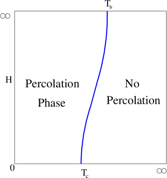
Figure 1: Schematic behaviour of the Kertész line for the Ising model

Turning now to the pseudocritical thermal behaviour of the models considered, we define the reduced temperature $t$ and external field $h$ measured relative to the spin-spin coupling strength

$$t=\frac{T-T_{c}}{T_{c}},\hskip 28.45274pth=\frac{H}{J}.$$ (5)

For spin systems, the renormalization group approach leads to the following expression of the magnetization $m$ when $t$, $h\,{\ll}\,1$

$$m\,=\,h^{1/\delta}f_{G}(t/h^{1/\beta\delta}),$$ (6)

where $f_{G}$ is a scaling function and $\beta$, $\delta$ are the critical exponents for the magnetization transition at $h=0$. We can rewrite Eq. (6) in the form

$$m\,=\,t^{\beta}({t/h^{1/\beta\delta}})^{-\beta}f_{G}(t/h^{1/\beta\delta})\,=\,t^{\beta}F_{G}(t/h^{1/\beta\delta})$$ (7)

with a new scaling function $F_{G}$; the entire dependence on the field $h$ is now put into the function $F_{G}$.

The susceptibility $\chi$ is given by

$$\chi\,\equiv\,\left(\frac{\partial{m}}{\partial{H}}\right)_{T}\,\propto\,t^{\beta}F_{G}^{\prime}(x)th^{-1/\beta\delta-1},$$ (8)

where $F_{G}^{\prime}(x)$ is the derivative of the function $F_{G}$ with respect to its argument $x=t/h^{1/\beta\delta}$. This time we move the dependence on the reduced temperature $t$ into a new function $\cal F$ of the argument $x$ and obtain

$$\chi\,\propto\,h^{1/\delta-1}{\cal F}(t/h^{1/\beta\delta})$$ (9)

To find the equation of the pseudocritical line, we have to determine the temperature $t_{\chi}(h)$ at which the susceptibility $\chi$ peaks for a given value $h$ of the field. Hence the derivative of $\chi$ with respect to the reduced temperature $t$ must vanish at $t=t_{\chi}$,

$$\frac{\partial{\chi}}{\partial{t}}\Big{|}_{t=t_{\chi}}\,=\,0\,\,\rightarrow\,\,h^{1/\delta-1}{\cal F}^{\prime}(x)|_{t=t_{\chi}}(1/h^{1/\beta\delta})\,=\,h^{1/\delta-1-1/\beta\delta}{\cal F}^{\prime}(x)|_{t=t_{\chi}}\,=\,0;$$ (10)

here ${\cal F}^{\prime}(x)|_{t=t_{\chi}}$ is the derivative of the function ${\cal F}$ with respect to its argument $x$ calculated at $t=t_{\chi}$. The derivative ${\partial{\chi}}/{\partial{t}}|_{t=t_{\chi}}$ can be zero only if ${\cal F}^{\prime}(x)|_{t=t_{\chi}}=0$. That will occur at some value $x_{\chi}$ of the argument $x=t_{\chi}/h^{1/\beta\delta}$, which provides the relation between $t_{\chi}$ and $h$

$$t_{\chi}/h^{1/\beta\delta}=x_{\chi}\,\,\rightarrow\,\,t_{\chi}\,\propto\,h^{1/\beta\delta}.$$ (11)

The procedure is obviously independent of the value of the field $h$, so that as long as $h$ is small, the pseudocritical line is described by a simple power law.

We stress that, for $h\rightarrow\infty$, the temperature of the susceptibility peak diverges, $t_{\chi}\rightarrow\infty$, whereas we have seen that the Kertész line has a finite endpoint, given by Eq. (3). Hence the two curves, which start from the same point but tend to two different limits, must certainly differ for sufficiently large values of $h$. We want to investigate here, however, what happens in the vicinity of the thermal critical point of the model, i.e. for small fields ($h\,{\approx}\,0$).

In order to study the percolation transition we need to redefine each given spin configuration as a cluster configuration, by grouping all spins of the lattice in clusters. We do this with the help of the algorithm of Hoshen and Kopelman [12], using free boundary conditions for the cluster identification and assuming that a cluster percolates if it connects each pair of opposite sides (faces in 3d) of the lattice.

After measuring the size of all clusters, i.e., the number of sites in each cluster, we evaluate the following two quantities:

• The average cluster size $S$,

  $$S\equiv\frac{\sum_{s}{{n_{s}s^{2}}}}{\sum_{s}{n_{s}s}}~{},$$ (12)

  where $n_{s}$ is the number of clusters of size $s$; the sums exclude the percolating cluster.

• The percolation strength $P$,

  $$P=\frac{\mbox{\rm size of the percolating cluster}}{\mbox{\rm total number of lattice sites}},~{}$$ (13)

  which is the order parameter of the percolation transition.

In the infinite volume limit, the percolation variables are described by simple power laws

$$P\,\propto\,(T_{p}-T)^{\beta_{p}}~{}~{}~{}(T<T_{p}),\hskip 28.45274ptS\,\propto\,|T-T_{p}|^{-\gamma_{p}}$$ (14)

sufficiently close to the critical threshold $T_{p}$.

In order to determine the critical point of the percolation transition, we exploit the properties of a further very useful variable. For finite lattice size, there can be spanning clusters even for temperatures $T>T_{p}$, and there are spin configurations at temperatures $T<T_{p}$ below the critical threshold without such clusters. The probability of finding a spanning cluster on a finite lattice of linear dimension $L$ at a temperature $T$ is a well-defined function, the percolation cumulant $\Pi(T,L)$ [13]. For $T\simeq T_{p}$ and large $L$, it behaves as

$$\Pi(T,L)\,=\,\Phi\Big{[}\Big{(}\frac{T-T_{p}}{T_{p}}\Big{)}\,L^{1/{\nu_{p}}}\Big{]}.$$ (15)

where $\nu_{p}$ is the critical exponent governing the divergence of the percolation correlation length. The function $\Pi(T,L)$ is not a genuine percolation variable, since it has a non-trivial meaning only on finite lattices. On an infinite lattice it reduces to a step function: it is zero for $T>T_{p}$ and unity for $T<T_{p}$. Nevertheless, its particular features make it a powerful tool to extract information about the critical properties of percolation. In particular, at $T=T_{p}$, $\Pi(T_{p},L)=\Phi(0)$ for any value of $L$. That means that if we calculate the percolation cumulant as a function of $T$ for different lattice sizes, all curves $\Pi(T,L)$ will cross at the critical temperature $T_{p}$. Moreover, if we plot the different $\Pi(T,L)$ as a function of the variable $X=[(T-T_{p})/T_{p}]L^{1/{\nu_{p}}}$, the resulting functions $\Phi(X)$ must coincide for all lattice sizes. To define the scaling function $\Phi(X)$, one also has to know the value of the exponent $\nu_{p}$. We can therefore determine $\nu_{p}$ by looking for the best scaling form of the percolation cumulant curves.

Let us now first consider the results obtained for the 2D Ising model. Our aim is to determine the functional form $t_{p}(h)$ describing the Kerteśz line. In order to compare it to the pseudocritical line, we have to perform simulations at small values of the reduced field $h$. We consider the following four values: $h$= 0.002, 0.001, 0.0005 and 0.00025. The Monte Carlo algorithm used in the simulations is the Wolff cluster update extended to the case of a non-vanishing external field [14]. For each iteration we have measured the energy $\epsilon$ of the configuration, its magnetization $m$, and the percolation variables $S$ and $P$. To determine the percolation critical point with a good accuracy, we work with rather large lattices: $300^{2}$, $500^{2}$, $700^{2}$, $1000^{2}$. This is helpful also for another reason. Since the field is quite weak, the scaling behaviour of both thermal and percolation variables could be perturbed by the “near-by” case of the system without field, which could affect the values of the critical exponents. Such perturbation becomes smaller the larger the size of the lattice.

Figure 2: Percolation cumulants for four lattice sizes; $\beta=J/kT$, $h$=0.00025.

Fig. 2 shows the percolation cumulants as a funtion of $\beta=J/kT$ for different lattice sizes, at the smallest field we have studied, $h=0.00025$. The curves cross clearly at the same point ($\beta_{p}=0.43933$). To check the universality class of the percolation exponents in this case, we rescale the percolation cumulants as discussed in Section 3. Using $J/kT_{p}=0.43933$, we consider two options for the critical exponent $\nu_{p}$, the 2-dimensional random percolation value $\nu_{RP}=4/3$ and the 2D Ising exponent $\nu_{IM}=1$. The results are shown in Figs. 4 and 4; they clearly indicate that the critical behaviour at the Kertész line is determined by the random percolation exponent $\nu_{RP}$, as expected.

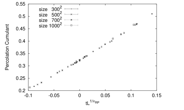
Figure 3: The rescaled percolation cumulants of Fig. 2 with $J/kT_{p}=0.43933$ and the 2-dimensional random percolation exponent $\nu_{RP}=4/3$.

Figure 4: The rescaled percolation cumulants of Fig. 2 with $J/kT_{p}=0.43933$ and the 2-dimensional Ising exponent $\nu_{IM}=1$.

Using a standard finite-size scaling analysis of the average cluster size $S$ near the critical point, we obtain for the ratio of the exponents $\gamma_{p}/\nu_{p}=1.80(2)$, in accord with the value predicted from the random percolation exponents (129/72=1.7916) and not with that from the Ising model (7/4=1.75). Repeating the percolation cumulant study for the other three values of $h$, we find the critical percolation temperatures listed in Table 1 and plotted in Fig. 5. In the Figure, the reduced percolation temperature $t_{p}=(T_{p}-T_{c})/T_{c}$ is shown as function of the external field; here $T_{c}$ is the critical temperature of the Ising model without field ($J/kT_{c}=(1/2)\log(\sqrt{2}+1)=0.44068679$). On the logarithmic scale of the plot the data points fall remarkably well on a straight line. We thus conclude that, for the Kertész line of the 2D Ising model,

$$t_{p}=a_{p}h^{\kappa},\hskip 14.22636pt{\rm for}~{}h\,{\rightarrow}\,0,$$ (16)

where $a_{p}$ is a constant of proportionality. From the slope in Fig. 5 we obtain $\kappa\,=\,0.534(3)$. On the other hand, the exponent of the thermal pseudocritical line is $1/\beta\delta$ (see Eq. (11)). For the 2D Ising model, $\beta=1/8$, $\delta=15$, so that $1/\beta\delta=8/15=0.533$. The agreement between this value and the exponent found for the Kertész line is excellent.

$h$	$J/kT_{p}$
0.00025	0.43933(3)
0.00050	0.43875(4)
0.00100	0.43786(4)
0.00200	0.43662(4)

Table 1: Percolation thresholds for the 2D Ising model at different values of the field.

Figure 5: Kertész line and pseudocritical line for the 2D Ising model.

Figure 6: Susceptibility $\chi$ for the $700^{2}$ and $1000^{2}$ lattices at $h=0.001$.

We thus ask ourselves whether the Kertész line and the pseudocritical line overlap in the range of $h$ values we have chosen. To answer this, we determine some points of the pseudocritical line and compare them to the corresponding points of the Kertész line. Fig. 6 shows the susceptibility as a function of $\beta$ for $h=0.001$, calculated on the two largest lattices we have studied. The curves are obtained by interpolating the data points using the density of state method [15]. The Figure clearly indicates that there is no noticeable change of the peak between $700^{2}$ to $1000^{2}$, so that we are effectively at the infinite volume limit. The position of the peak in the Figure, however, clearly differs from the corresponding percolation point at $h=0.001$, indicated by the dotted line.

To complete the comparison, we determine the positions of the susceptibility peaks for two other values of the field, $h=0.0005$ and $h=0.002$. As above, we find clear discrepancies with the corresponding points of the Kertész line; the results are included in Fig. 5, where it is also seen that the power law of Eq. (11)

$$t_{\chi}=a_{\chi}h^{1/\beta\delta},~{}~{}a_{\chi}={\rm const.}$$ (17)

continues to be valid with great precision. We conclude that for the 2D Ising model the functional dependence of the reduced temperature $t$ on the field $h$ for $h{\rightarrow}0$ is for the Kertész line and for the pseudocritical line described by the same function, determined by the thermal critical exponent $1/\beta\delta$; but the two curves do not coincide, since $a_{p}\not=a_{\chi}$, as is evident in Fig. 5.

We now turn to the corresponding study of the 3D $O(2)$ model. Here we have determined four points of the Kertész line, for external field $h$ values 0.001, 0.00050, 0.00025, and 0.000125, using again the cluster update [14] as Monte Carlo algorithm, on lattices of size $30^{3}$, $40^{3}$, $50^{3}$, $60^{3}$, $70^{3}$, $80^{3}$, $100^{3}$. The clusters we considered are those used in the Wolff algorithm with no external field (see [6, 16]).

The positions of the percolation points, determined as before by the crossing of the percolation cumulant curves, are listed in Table 2. As for the Ising model, we have checked that the universality class of the exponents of each percolation transition is that of random percolation, here in three dimensions. We show these points in Fig. 7, again plotting the $h$-dependence of the reduced percolation temperature $t_{p}\,=\,(T_{p}-T_{c})/T_{c}$. The critical temperature $T_{c}$ of the magnetization transition for the 3D $O(2)$ model without field was found to be $J/kT_{c}=0.454165$ in [17].

$h$	$J/kT_{p}$
0.000125	0.45312(2)
0.000250	0.45257(2)
0.000500	0.45178(3)
0.001000	0.45053(3)

Table 2: Percolation thresholds for the 3D $O(2)$ model at different values of the field.

Figure 7: Kertész line and pseudocritical line for the 3D $O(2)$ model.

Again, the straight line in the log-log plot clearly indicates the power law behaviour of the Kertész line. The slope of the straight line is $0.601(3)$, in good agreement with the exponent of the pseudocritical line $1/\beta\delta=0.5995(6)$, obtained by using the $O(2)$ thermal exponents values determined in [18].

To compare the two lines directly, we make use of the results of a recent numerical determination of the $O(2)$ pseudocritical line [19]. The results are included in Fig. 7. The two lines are parallel in the log-log plot, since the exponents of $h$ agree, but they do not coincide.

We have shown that the Kertész lines of the 2D Ising model and the 3D $O(2)$ model are in the limit of small fields described by the same functions as the corresponding thermal pseudocritical lines, i.e., a power law with exponent $1/\beta\delta$. This feature, which is likely to be general, suggests a relationship between the geometrical percolation singularities which still occur for $H{\neq}0$ and the remaining non-singular thermal properties of the system. In both models we have found that the Kertész line does not coincide with the pseudocritical line even in the scaling region we have explored. The difference in the behaviour of the two lines could well be a consequence of using the conventional $h=0$ bond weight (2) also for $h\not=0$; introducing a dependence on the field $h$ into the Coniglio-Klein factor might well make the two lines coincide. Simple expressions of the form $1-\exp[-2\beta(1+h)]$ would lead to a Kertész line which goes to infinity for $h\,\rightarrow\infty$, so that an eventual interpretation of the pseudocritical line as a curve of percolation points is not yet excluded. Further work on this is in progress.

Acknowledgements

It is a pleasure to thank J. Engels for helpful discussions. We would also like to thank the TMR network ERBFMRX-CT-970122 and the DFG Forschergruppe Ka 1198/4-1 for financial support.

References

- [1] D. Stauffer, A. Aharony, Introduction to Percolation Theory, Taylor & Francis, London 1994.
- [2] G. R. Grimmett, Percolation, Springer-Verlag, 1999.
- [3] A. Coniglio, W. Klein, J. Phys. A 13, 2775 (1980).
- [4] P. Bialas et al., Nucl. Phys. B 583, 368 (2000).
- [5] S. Fortunato, H. Satz, Nucl. Phys. B 598, 601 (2001).
- [6] P. Blanchard et al., J. Phys. A 33, 8603 (2000).
- [7] J. Kertész, Physica A 161, 58 (1989).
- [8] H. Satz, Phase Transitions in QCD, Proceedings of the Catania Relativistic Ion Studies (CRIS 2000), Acicastello (Italy).
- [9] J. Adler, D. Stauffer, Physica A 175, 222 (1991).
- [10] X. Campi, H. Krivine, Nucl. Phys. A 620, 46 (1997).
- [11] X. Campi, H. Krivine, N. Sator, cond-mat/0005348.
- [12] J. Hoshen, R. Kopelman, Phys. Rev. B 14, 3438 (1976).
- [13] K. Binder, D. W. Heermann, Monte Carlo Simulations in Statistical Physics, An Introduction, Springer-Verlag, 40-41 (1988).
- [14] I. Dimitrović et al., Nucl. Phys. B 350, 893 (1991).
- [15] M. Falcioni et al., Phys. Lett. B 108, 331 (1982); E. Marinari, Nucl. Phys. B 235, 123 (1984); G. Bhanot et al., Phys. Lett. B 183, 331 (1986); A. M. Ferrenberg, R. H. Swendsen, Phys. Rev. Lett. 61, 2635 (1988), and 63, 1195 (1989).
- [16] U. Wolff, Phys. Rev. Lett. 62, 361 (1989).
- [17] H.G. Ballesteros, L. A. Fernandez, V. Martín-Major, A. Munõz Sudupe, Phys. Lett. B 387, 125 (1996).
- [18] M. Hasenbusch, T. Török, J. Phys. A 32, 6361 (1999).
- [19] J. Engels et al., Nucl. Phys. Proc. Suppl. 94, 861 (2000).