STUDYING HADRONIC STRUCTURE OF THE PHOTON
IN LATTICE QCD

Abstract

We show that the matrix element of a local quark-gluon operator in the photon state, $\langle\gamma(k\lambda)|\hat{O}|\gamma(k\lambda)\rangle$, can be calculated in lattice QCD. The result is generalized to other quantities involving space-like photons, including the transition form factor $\gamma\gamma^{*}\rightarrow\pi^{0}$ and the virtual-photon-nucleon Compton amplitude $\langle\gamma^{*}N|\gamma^{*}N\rangle$ which can be used to define the generalized Drell-Hearn-Gerasimov and Bjorken sum rules.

Ever since the 1960’s, it has been well known that the photon is not just a point-like particle; rather, it has a complicated hadronic structure. Similarity of the photon-nucleon scattering cross section to that of meson-nucleon scattering has led to the so-called vector dominance model of photon-hadron interactions [1]. In recent years, the photon structure has been explored extensively in $e^{+}e^{-}$ and $ep$ collider experiments [2]. For instance, in the certain kinematic region, $e^{+}e^{-}$ scattering is effectively the real and deeply-virtual photon collision, from which the partonic structure of the real photon can be extracted. Indeed, the unpolarized quark and gluon distributions in the photon has been phenomenologically determined to a reasonable accuracy [2], and future data from the polarized HERA and $e^{+}e^{-}$ colliders can constrain the polarized distributions as well [3].

Given the large amount of experimental data available to describe the hadronic properties of the photon, it is appropriate to ask how they can be understood from the fundamental theory— quantum chromodynamics (QCD). To the authors’ knowledge, the answer is still open. Part of the reason is that the photon is not an eigenstate of QCD; the standard lattice QCD method used in calculating the matrix elements of the nucleon and pion does not apply [4]. As we shall explain, the QCD matrix elements in the photon state are time-dependent correlations which are notoriously difficult to access through the Euclidean space [5]. However, we will show in this paper that they can be extracted from the Euclidean correlation functions on a lattice. In particular, the moments of polarized (unpolarized) quark and gluon distributions of the photon can be calculated in Monte Carlo simulations just like for those of the nucleon. Generalizing our finding, we show that a number of processes involving space-like virtual photons, such as transition $\gamma\gamma^{*}\rightarrow\pi$ [6] and the virtual-photon-nucleon forward Compton scattering $\gamma^{*}N\rightarrow\gamma^{*}N$, can be studied in lattice QCD. The amplitude for the latter process is the key for generalizing the well-known Drell-Hearn-Gerasimov and Bjorken sum rules for the spin-dependent structure function of the nucleon [7].

We start with a simple but instructive discussion about what is meant by the hadronic or QCD structure of the photon. If $\hat{O}(0)$ is a quark-gluon operator at the spacetime point 0, its matrix element in the photon state can be defined from the standard Lehmann-Symanzik-Zimmermann (LSZ) reduction formula,

$$\langle\gamma(k\lambda^{\prime})|\hat{O}(0)|\gamma(k\lambda)\rangle=-\lim_{k^{\prime\mu}\rightarrow k^{\mu}}\int d^{4}xd^{4}ye^{-ik^{\prime}(y-x)}k^{\prime 2}\langle 0|T\epsilon^{*}(\lambda^{\prime})\cdot A(x)~{}\hat{O}(0)~{}\epsilon(\lambda)\cdot A(y)|0\rangle k^{\prime 2}\ ,$$ (1)

where $k^{\mu}$ is the on-shell ($k^{2}=0$) photon momentum, $\lambda$ and $\lambda^{\prime}$ are the photon helicities, and $k^{\prime\mu}$ on the right-hand side is taken to be on-shell after cancelling the photon poles. The normalization for the photon states are taken to be covariant, i.e., $\langle\gamma(k^{\prime}\lambda^{\prime})|\gamma(k\lambda)\rangle=2k^{0}(2\pi)^{3}\delta(\vec{k}^{\prime}-\vec{k})\delta_{\lambda\lambda^{\prime}}$. The renormalization constant $Z_{3}=1+{\cal O(\alpha_{\rm em})}$ has been omitted for simplicity. Evaluating the electromagnetic part of the Green’s function in the lowest-order perturbation theory (this is allowed because of the small electromagnetic coupling), we find

$$\langle\gamma(k\lambda^{\prime})|\hat{O}(0)|\gamma(k\lambda)\rangle=-e^{2}\int d^{4}xd^{4}ye^{-ik(y-x)}\epsilon^{*\mu}(\lambda^{\prime})\langle 0|TJ_{\mu}(x)\hat{O}(0)J_{\nu}(y)|0\rangle\epsilon^{\nu}(\lambda)\ ,$$ (2)

where $e$ is the renormalized electric charge unit and $J^{\mu}$ is the electromagnetic current operator of the quarks. According to the above equation, the matrix element of interest is a Minkowski-space correlation function in QCD. This is in contrast to an analogous nucleon matrix element, $\langle p|\hat{O}|p\rangle$, which has no explicit reference to the Minkowski time.

One can remove the explicit time dependence by deriving a Lehmann representation of Eq. (2): separating different time-orderings, inserting complete sets of hadronic states, and integrating out the spacetime coordinates $x$ and $y$. The result can be shown as the time-independent perturbation diagrams in Fig. 1. Diagrams a) to f) represent contributions from six possible time-orderings. Diagrams g) to i) are the vacuum contributions which must be subtracted. As an example, the diagram a) corresponds to the following time-independent matrix element,

$$\langle\gamma(k\lambda^{\prime})|\hat{O}(0)|\gamma(k\lambda)\rangle_{\rm Fig.~{}1a}=e^{2}\sum_{nn^{\prime}}{\langle 0|\epsilon^{*}(\lambda^{\prime})\cdot J(\vec{k})|n^{\prime}\rangle\langle n^{\prime}|\hat{O}(0)|n\rangle\langle n|\epsilon(\lambda)\cdot J(\vec{k})|0\rangle\over(\omega-E_{n})(\omega-E_{n^{\prime}})}\ ,$$ (3)

where $|n\rangle$ are the eigenstates of $H_{\rm QCD}$ with momentum $\vec{k}$, and $\omega=|\vec{k}|$ is the on-shell photon energy. The contributions from the other diagrams can be expressed similarly using the rules from time-independent perturbative theory.

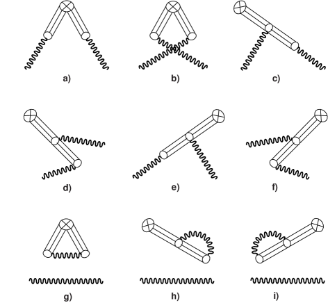
FIG. 1.: Time-ordered diagrams for the quark-gluon matrix elements of the photon state. The circles with crosses represent local quark and gluon operators, and the open ones the electromagnetic currents. Multiple parallel lines indicate the intermediate hadronic eigenstates.

Though hardly new, the Lehmann representation helps us in understanding the physical origin of the vector dominance. With certain probability, the photon is a superposition of a set of hadron states with the photon quantum numbers. The lowest-lying such states are $\pi\pi$ scattering states in the $p$-wave. A strong resonance in this channel is the $\rho$ meson. The vector dominance then refers to the dominance of the $\rho$ resonance in the above hadron-state summations, although other hadron states can and do contribute. It is interesting to note from Fig. 1 that the hadronic part of the photon wave function does not consist of just the pure hadron states; it contains also the components that are the mixtures of one or more resolved photons and hadrons.

The above discussion makes it clear that the hadronic structure of the photon is qualitatively different from that of ordinary hadrons, at least in the context of QCD. The photon matrix elements contain explicit sums over the complete set of QCD eigenstates as well as the contributions from different time-orderings. Because the time-dependent correlation functions are generically difficult to study in the Euclidean space, there are no general rules to calculate them in lattice QCD. One might be tempted to use the electromagnetic current $J^{\mu}$ as a photon interpolating field to extract the matrix element of interest from $\langle 0|J_{\mu}(y)\hat{O}(0)J_{\nu}(x)|0\rangle$ at large positive $-x_{4},y_{4}$. The actual outcome is a matrix element between the threshold two-$\pi$ states, or the $\rho$ if it were stable.

The key observation for a lattice calculation of the photon matrix element is that the photon is an eigenstate of the combined eletromagnetic and strong interaction hamiltonian [8]. When both interactions are present, we can use the electromagnetic potential $A^{\mu}$ as the interpolating field for photon. Thus we consider the following matrix elements in the Euclidean space,

$$\langle 0|A_{\mu}(y)\hat{O}(0)A_{\nu}(x)|0\rangle\ ,$$ (4)

where $x$ and $y$ are Euclidean coordinates. After Fourier-transforming the spatial coordinates and letting $y_{4}$ and $-x_{4}$ be large, we have

$$M_{\mu\nu}( y_{4} ,x_{4},\vec{k})=\int d^{3}\vec{x}e^{-i{\vec{k}}\cdot\vec{x}}\int d^{3}\vec{y}e^{i\vec{k}\cdot\vec{x}}\langle 0|A_{\mu}(\vec{y},y_{4})\hat{O}(0)A_{\nu}(\vec{x},x_{4})|0\rangle$$ (6)

$$\rightarrow\sum_{\lambda\lambda^{\prime}}\langle 0|A_{\mu}(\vec{k})|\gamma(k\lambda^{\prime})\rangle e^{-y_{4}\omega}\langle\gamma(k\lambda^{\prime})|\hat{O}(0)|\gamma(k\lambda)\rangle e^{x_{4}\omega}\langle\gamma(k\lambda)|A_{\nu}(\vec{k})|0\rangle\ .$$

The summations over $\lambda$ and $\lambda^{\prime}$ can be selected by multiplying $M_{\mu\nu}$ with appropriate polarization vectors. In the second line, we have neglected the three-photon states with the same momentum which are suppressed by powers of $\alpha_{\rm em}$, and the hadronic states which are suppressed by an energy gap ($2m_{\pi}$ at $\vec{k}\sim 0$).

Before putting $M_{\mu\nu}(y_{4},x_{4},\vec{k})$ on a lattice, we integrate out the photon field in perturbation theory,

$$M_{\mu\nu}(y_{4},x_{4},\vec{k}) = e^{2}\int d^{4}wd^{4}ze^{-i\vec{k}\cdot(\vec{w}-\vec{z})}D_{\mu\rho}(\vec{k},y_{4}-w_{4})$$ (8)

$$\times\langle 0|T_{E}J_{\rho}(\vec{w},w_{4})\hat{O}(0)J_{\sigma}(\vec{z},z_{4})|0\rangle D_{\sigma\nu}(\vec{k},z_{4}-x_{4})\ ,$$

where $D^{\mu\nu}$ is the photon propagator in the Euclidean space and $T_{E}$ is the Euclidean time-ordering. Using the Fourier integral ($k>0$),

$$\int^{\infty}_{-\infty}d\omega{e^{i\omega z}\over\omega^{2}+k^{2}}={\pi\over k}e^{-k|z|}\ ,$$ (9)

we can write

$$M_{\mu\nu}(y_{4},x_{4},\vec{k})\sim\int dw_{4}dz_{4}e^{-\omega|z_{4}-x_{4}|}e^{-\omega|y_{4}-w_{4}|}\langle 0|T_{E}J_{\mu}(-\vec{k},w_{4})\hat{O}(0)J_{\nu}(\vec{k},z_{4})|0\rangle\ .$$ (10)

Taking the limit $y_{4},-x_{4}\rightarrow\infty$ and comparing the result with Eq. (6), we get,

$$\langle\gamma(k\lambda^{\prime})|\hat{O}(0)|\gamma(k\lambda)\rangle=e^{2}\int dw_{4}dz_{4}e^{\omega(w_{4}-z_{4})}\epsilon^{*}_{i}(\lambda^{\prime})\langle 0|T_{E}J_{i}(-\vec{k},w_{4})\hat{O}(0)J_{j}(\vec{k},z_{4})|0\rangle\epsilon_{j}(\lambda)\ ,$$ (11)

where we have restored the photon polarization in physical gauge ($\epsilon^{0}=0$ and $\vec{\epsilon}\cdot\vec{k}=0$), $i$ and $j$ sum over spatial indices, and $J_{\mu}=\sum_{f}e_{f}\bar{\psi}_{f}\gamma_{\mu}\psi_{f}$ is the electromagnetic current summing over all quark flavors $f$. The above equation is one of the main results of this paper.

Several comments on Eq. (11) are as follows: First, the Euclidean correlation function $\langle 0|T_{E}J^{\mu}(\vec{k},w_{4})\hat{O}(0)J^{\nu}(\vec{k},z_{4})|0\rangle$ can be calculated in the standard Monte Carlo simulations. Hence, the photon matrix elements are accessible in lattice QCD just like the nucleon ones. Second, the above expression is nothing but a straightforward analytical continuation of the expression in Eq. (2). However, the process arriving at Eq. (11) makes it clear that the analytical continuation fails if there is no energy gap between the photon and hadronic states. Finally, $\langle 0|TJ_{\mu}(\vec{k},w_{4})\hat{O}(0)J_{\nu}(\vec{k},z_{4})|0\rangle$ is what one would naively consider when using $J^{\mu}$ as a photon interpolating field. On the other hand, the correct result involves integrations over $w_{4}$ and $z_{4}$, which include not only the lowest-energy hadron state but all others with the photon quantum numbers. Finally, it is straightforward to show that the above Euclidean correlation function reproduces the Lehmann representation of the photon matrix element. In the process, one finds that if the energy of the photon exceeds that of the lowest hadronic state (the gap vanishes), Eq. (11) is divergent. Thus, we emphasize that the photon matrix element is calculable on a lattice only when there is an energy gap between the photon and hadron states.

In the remainder of the paper, we explore under what conditions the above result can be generalized. First of all, the initial and final photons can have different 3-momenta, and then the forward matrix element is generalized to form factors. Next, we introduce the hadronic structure of an off-shell photon for which $\omega\neq|\vec{k}|$. The parton distributions in an off-shell photon can be extracted from experimental data just as for an on-shell photon [2]. In QCD, the off-shell photon matrix elements are defined in terms of the same Minkowski correlation in Eq. (2). The corresponding Euclidean expression in Eq. (11) is valid only when $0<\omega<\sqrt{4m_{\pi}^{2}+\vec{k}^{2}}$, where the upper limit refers to the hadron production threshold for a time-like photon. Finally, one can define and calculate on a lattice the hadronic matrix elements of the weak-interaction gauge bosons, off- or on-shell, by replacing in Eq. (11) the electromagnetic currents with the weak-interaction currents.

To make further progress, we explore under what conditions a Minkowski correlation can be obtained from a numerical calculation of the corresponding Euclidean correlation. Euclidean Green’s functions are generally real as they can be expressed as real integrals in the functional formulation and amenable to Monte Carlo simulations, whereas Minkowski correlations can have imaginary parts corresponding to physical intermediate states propagating infinite distances. Therefore, it is reasonable to expect that Minkowski correlations can be analytically continued and calculated in Euclidean space only when they are in kinematic domains where no physical intermediate states are allowed. In the example of the matrix elements for an off-shell photon, the condition $\omega<\sqrt{4m_{\pi}^{2}+\vec{k}^{2}}$ ensures that the photon can never turn into a real hadron state.

Thus the transition form factor (amplitude) corresponding to $\gamma\gamma^{*}\rightarrow\pi^{0}$ is calculable on a lattice, where the first photon is real and the second is space-like. In Minkowski space the amplitude can be expressed as

$$A_{\mu\nu}(P,k)=\int d^{4}ye^{iky}\langle 0|TJ_{\mu}(y)J_{\nu}(0)|\pi(P)\rangle\ .$$ (12)

Denoting the interpolating field for the pion as $\phi$, we construct the following Green’s function in the Euclidean space,

$$G_{\mu\nu}(\vec{P},x_{4},k)=\int dy_{4}e^{y_{4}\omega}\langle 0|T_{E}J_{\mu}(\vec{k},y_{4})J_{\nu}(0)\phi(\vec{P},x_{4})|0\rangle\ .$$ (13)

Taking $x_{4}\rightarrow-\infty$ and keeping only the pion state of momentum $\vec{P}$, we have

$$G_{\mu\nu}(\vec{P},x_{4},k)=\int dy_{4}e^{y_{4}\omega}\langle 0|T_{E}J_{\mu}(\vec{k},y_{4})J_{\nu}(0)|\pi(P)\rangle e^{x_{4}E_{P}}\langle\pi(P)|\phi(\vec{P})|0\rangle\ ,$$ (14)

where $E_{P}=\sqrt{\vec{P}^{2}+m_{\pi}^{2}}$ is the on-shell pion energy. By working out its Lehmann representation, the Euclidean correlation function reproduces the corresponding Minkowski amplitude.

The final example involving the photons is the forward virtual-photon-nucleon Compton scattering amplitude,

$$T_{\mu\nu}(P,q)=i\int e^{iqx}d^{4}x\langle P|TJ_{\mu}(x)J_{\nu}(0)|P\rangle\ ,$$ (15)

where $|P\rangle^{\mu}$ is the nucleon state with momentum $P$. The space-like virtual photon momentum has two distinct kinematic regions, $(P+q)^{2}>M_{N}^{2}$ and $(P+q)^{2}<M_{N}^{2}$, where $M_{N}$ is the nucleon mass. In the former region, the amplitude is complex and its imaginary part corresponds to the inclusive production cross section in $eP$ scattering. In the other region, the Compton amplitude is real and therefore we expect it is calculable in lattice QCD. Define the four-point Euclidean correlation,

$$G_{\mu\nu}(\vec{P},y_{4},z_{4},\vec{q})=\int dx_{4}e^{x_{4}\omega}\langle 0|T_{E}\eta(\vec{P},y_{4})J_{\mu}(\vec{q},x_{4})J_{\nu}(0)\bar{\eta}(\vec{P},z_{4})|0\rangle\ ,$$ (16)

where $\eta$ is an interpolating field for the nucleon. Take the limit $y_{4},-z_{4}\rightarrow\infty$, we have the nucleon state dominance,

$$G_{\mu\nu}(\vec{P},y_{4},z_{4},\vec{q})=\int dx_{4}e^{x_{4}\omega}\langle 0|\eta(\vec{P})|P\rangle e^{-y_{4}E_{P}}\langle P|T_{E}J_{\mu}(\vec{q},x_{4})J_{\nu}(0)|P\rangle e^{z_{4}E_{P}}\langle P|\bar{\eta}(\vec{P})|0\rangle\ .$$ (17)

Integrating over $x_{4}$, we find that the remaining correlation function reproduces the physical Compton amplitude in the region $(P+q)^{2}<M_{N}^{2}$.

A particularly interesting application is when $\omega=0$. The spin-dependent Compton amplitude as a function of $Q^{2}=-q^{2}$ defines an integral over $\nu$ for the $G_{1}(\nu,Q^{2})$ structure function of the nucleon. In the limit $Q^{2}\rightarrow 0$, the amplitude can be obtained by the low-energy theorem and chiral perturbation theory and the integral defines the Drell-Hearn-Gerasimov sum rule and its generalization [7]. In the limit $Q^{2}\rightarrow\infty$, the amplitude can be studied in perturbative QCD and the integral defines the Bjorken sum rule and its generalization. Our result here allows a lattice QCD calculation of the amplitude at intermediate $Q^{2}$ where there is no firm theoretical prediction available.

In conclusion, we have shown that the QCD structure of the photon can be studied on a lattice by calculating Euclidean correlation functions involving local quark-gluon operators and electromagnetic currents. Also calculable are a number of other interesting examples involving photons, such as $\gamma\gamma^{*}\rightarrow\pi^{0}$ and $\gamma^{*}N\rightarrow\gamma^{*}N$. These results shall lead to more exciting interplay between lattice QCD and strong-interaction phenomenology.

- [1] J. Sakurai, Ann. Phys. (N. Y.) 11, 1 (1960); Currents and Mesons (University of Chicago Press, 1969); D. Leith, in Electromagnetic Interactions of Hadrons, Vol. 1, eds. A. Donnachie and G. Shaw (Plenum Press, New York, 1978).
- [2] For a compilation of data, see R. Nisius, Phys. Rept. 332, 165 (2000).
- [3] M. Stratmann, hep-ph/9910318; hep-ph/9907467; M. Stratmann and W. Vogelsang, Phys. Lett. B386, 370 (1996).
- [4] See for instance, J. Negele, hep-lat/9804017; S. J. Dong, J. F. Lagae, K. F. Liu, Phys. Rev. Lett. 75, 2096 (1995).
- [5] L. Maiani and M. Testa, Phys. Lett. B245, 585 (1990).
- [6] G. P. Lepage and S. J. Brodsky, Phys. Rev. D22, 2157 (1980); A. V. Radyushkin, Nucl. Phys. B481, 625 (1996).
- [7] X. Ji and Osborne, hep-ph/9905410; X. Ji, C. Kao, and J. Osborne, Phys. Lett. B472, 1 (2000).
- [8] A. Mueller, private communication.