Infinite Volume and Continuum Limits of the Landau-Gauge Gluon Propagator

Abstract

We extend a previous improved action study of the Landau gauge gluon propagator, by using a variety of lattices with spacings from $a=0.17$ to 0.41 fm, to more fully explore finite volume and discretization effects. We also extend a previously used technique for minimizing lattice artifacts, the appropriate choice of momentum variable or “kinematic correction”, by considering it more generally as a “tree-level correction”. We demonstrate that by using tree-level correction, determined by the tree-level behavior of the action being considered, it is possible to obtain scaling behavior over a very wide range of momenta and lattice spacings. This makes it possible to explore the infinite volume and continuum limits of the Landau-gauge gluon propagator.

I Introduction

There has long been interest in the infrared behavior of the gluon propagator as a probe into the mechanism of confinement [1] and lattice studies focusing on its ultraviolet behavior have been used to calculate the running QCD coupling [2]. In this report we use the propagator as a test-bed for an improved action and also as a means to investigate a general tree-level correction technique.

The infrared part of any lattice calculation may be affected by the finite volume of the lattice. Larger volumes mean either more lattice points (with increased computational cost) or coarser lattices (with corresponding discretization errors). Improved actions have been shown to be effective at reducing discretization errors at a given lattice spacing in studies of the static quark potential [3] and the hadron spectrum [4] and have become a necessary part of finite temperature studies [5]. The desire for larger physical volumes thus provides strong motivation for using improved actions. We study the gluon propagator, in Landau gauge, in quenched QCD (pure SU(3) Yang-Mills), using the mean-field (tadpole) improved [6] version of the tree-level, ${\cal O}(a^{2})$ Symanzik improved gauge action [7, 8, 9].

To assess the effects of finite lattice spacing, we calculate the propagator on a set of lattices from $8^{3}\times 16$ at $\beta=3.75$ having $a=0.413$ fm to $16^{3}\times 32$ at $\beta=4.38$ having $a=0.167$ fm. To assist us in observing possible finite volume effects, we add to this set a $16^{3}\times 32$ lattice at $\beta=3.92$ with $a=0.353$, which has the very large physical size of $5.65^{3}\times 11.30\text{ fm}^{4}$. Some preliminary results of this work were reported in Ref. [10].

We will show that tree-level correction reduces rotational symmetry breaking and dramatically improves the ultraviolet behavior of the propagator and thus the approach to the continuum limit. For lattices as coarse as 0.17 fm the gluon propagator has surprisingly good behavior for the entire range of available momenta. The infrared behavior of the gluon propagator is robust even with an extremely coarse lattice spacing of 0.41 fm. Our calculations on a lattice with a large volume indicates that finite volume effects are small. The Landau gauge gluon propagator is again found to be infrared finite, in agreement with earlier studies. The combination of an improved action with appropriate tree-level correction appears to be a powerful tool. The generalization of these methods to the study of other Green’s functions will be discussed in a forthcoming work [11].

II The Landau gauge gluon propagator

We employ the tree-level, mean-field improved gauge action of Lüscher and Weisz [8, 9]

$$S_{\text{l}} = \frac{5\beta}{3N_{c}}\sum_{\text{pl}}\text{Tr}\Bigl{\{}1-\frac{1}{2}\bigl{(}P_{\mu\nu}+P_{\mu\nu}^{\dagger}\bigr{)}\Bigr{\}}-\frac{\beta}{12N_{c}u_{0}^{2}}\sum_{\text{rect}}\text{Tr}\Bigl{\{}1-\frac{1}{2}\bigl{(}R_{\mu\nu}+R_{\mu\nu}^{\dagger}\bigr{)}\Bigr{\}}$$ (1)

$$= S_{\text{cont}}+{\cal O}(a^{4})+{\cal O}(a^{2}g^{2}),$$ (2)

where $P_{\mu\nu}$ and $R_{\mu\nu}$ are the usual plaquette and rectangle operators

$$P_{\mu\nu}(x)=U_{\mu}(x)U_{\nu}(x+\hat{\mu})U_{\mu}^{\dagger}(x+\hat{\nu})U_{\nu}^{\dagger}(x)$$ (3)

and

$$R_{\mu\nu}(x) = U_{\mu}(x)U_{\nu}(x+\hat{\mu})U_{\nu}(x+\hat{\nu}+\hat{\mu})U^{\dagger}_{\mu}(x+2\hat{\nu})U^{\dagger}_{\nu}(x+\hat{\nu})U^{\dagger}_{\nu}(x)$$ (5)

$$+U_{\mu}(x)U_{\mu}(x+\hat{\mu})U_{\nu}(x+2\hat{\mu})U^{\dagger}_{\mu}(x+\hat{\mu}+\hat{\nu})U^{\dagger}_{\mu}(x+\hat{\nu})U^{\dagger}_{\nu}(x),$$

and $N_{c}=3$ is the number of colors. We use the plaquette definition for the tadpole factor

$$u_{0}=\left(\frac{1}{N_{c}}{\cal R}e{\rm Tr}\langle P_{\mu\nu}\rangle\right)^{\frac{1}{4}}.$$ (6)

Our gauge field configurations were generated using the Cabbibo-Marinari [12] pseudo-heatbath algorithm with appropriate link partitioning [13].

Given that the gauge links $U_{\mu}(x)$ are expressed in terms of the continuum gluon fields as

$$U_{\mu}(x)={\cal P}e^{ig\int_{0}^{1}A_{\mu}(x+at\hat{\mu})dt},$$ (7)

the dimensionless lattice gluon field $A_{\mu}(x)$ may be obtained from

$$A_{\mu}(x+\hat{\mu}/2)=\frac{1}{2igu_{0}}\bigl{\{}U_{\mu}(x)-U_{\mu}^{\dagger}(x)\bigr{\}}_{\text{traceless}}$$ (8)

which is accurate to ${\cal O}(a^{2})$. This is, of course, only one of many possible ways to calculate the gluon field on the lattice. In Eq. (8), $A_{\mu}$ is calculated at the midpoint of the link to remove ${\cal O}(a)$ terms. Note that we have also included the tadpole factor to improve the normalization.

We calculate the gluon propagator in coordinate space

$$D_{\mu\nu}^{ab}(x,y)\equiv\langle\,A_{\mu}^{a}(x)\,A_{\nu}^{b}(y)\,\rangle\,,$$ (9)

using Eq. (8). To improve statistics, we use translational invariance and calculate

$$D_{\mu\nu}^{ab}(y)=\frac{1}{V}\bigl{\langle}\sum_{x}A_{\mu}^{a}(x)A_{\nu}^{b}(x+y)\bigr{\rangle}.$$ (10)

The quantity that will be of interest to us is the scalar part of the propagator in momentum space, so first we take the trace over color components

$$D_{\mu\nu}(y)=\frac{1}{N_{c}^{2}-1}\sum_{a}D_{\mu\nu}^{aa}(y),$$ (11)

then sum over the Lorentz components of the Fourier transform

$$D(\hat{q})=\frac{1}{N_{d}-1}\sum_{\mu}\sum_{y}e^{i\hat{q}\cdot y}D_{\mu\mu}(y)$$ (12)

and

$$D(0)=\frac{1}{N_{d}}\sum_{\mu}\sum_{y}D_{\mu\mu}(y).$$ (13)

$N_{d}$ is the number of space-time dimensions and the available momentum values, $\hat{q}$, are given by

$$\hat{q}_{\mu}=\frac{2\pi n_{\mu}}{aL_{\mu}},\qquad n_{\mu}\in\Bigl{(}-\frac{L_{\mu}}{2},\frac{L_{\mu}}{2}\Bigr{]}.$$ (14)

The range of $\hat{q}$ is determined by the fact that our lattices have an even number of points in each direction and that we use periodic boundary conditions. In the continuum, the scalar propagator is related to the full propagator by

$$D_{\mu\nu}^{ab}(q)=\bigl{(}\delta_{\mu\nu}-\frac{q_{\mu}q_{\nu}}{q^{2}}\bigl{)}\delta^{ab}D(q^{2})$$ (15)

in Landau gauge.

Landau gauge is a smooth gauge that preserves the Lorentz invariance of the theory, so it is a popular choice. We work in Landau gauge for ease of comparison with other studies, and because it is the simplest covariant gauge to implement on the lattice. All configurations were gauge fixed by maximizing an ${\cal O}(a^{2})$ improved Landau gauge fixing functional using Conjugate Gradient Fourier Acceleration [15] as described in Ref. [16].

III Tree-level Correction

One thing that is known about the gluon propagator is its perturbative, asymptotic behavior. In the spirit of improvement, we can use this knowledge to augment our lattice results and make better contact with the continuum. In the continuum, as $p^{2}\rightarrow\infty$, the propagator has the form

$$D(p)=\frac{1}{p^{2}}$$ (16)

up to logarithmic corrections. A well known artifact of the lattice is that for a free massless boson with an unimproved action the lattice propagator has the form

$$D(\hat{q})=\frac{1}{\frac{4}{a^{2}}\sum_{\mu}\sin^{2}\bigl{(}\frac{\hat{q}_{\mu}a}{2}\big{)}}.$$ (17)

It has been argued, in Ref. [17] and elsewhere, that the correct momentum variable to use when examining the gluon propagator on the lattice, with the Wilson action, is not Eq. (14), but

$$q_{\mu}\equiv\frac{2}{a}\sin\frac{\hat{q}_{\mu}a}{2}.$$ (18)

It has been observed that this choice ensures that the propagator takes its asymptotic form at large lattice momenta [17, 18].

The improved action Eq. (2) together with the gluon field defined in Eq. (8) has the ${\cal O}(a^{2})$ improved tree-level behavior [7, 8]

$$D^{-1}(\hat{q})=\frac{4}{a^{2}}\sum_{\mu}\biggl{\{}\sin^{2}\Bigl{(}\frac{\hat{q}_{\mu}a}{2}\Bigr{)}+\frac{1}{3}\sin^{4}\Bigl{(}\frac{\hat{q}_{\mu}a}{2}\Bigr{)}\biggr{\}},$$ (19)

and we will use Eqs. (17) and (19) to obtain the correct momentum variable for each action. To emphasize the nonperturbative aspects of the propagator, we divide it by its perturbative, $1/q^{2}$ result. Hence, all figures are plotted against $q^{2}D(q^{2})$, which is expected to approach a constant up to logarithmic corrections as $q^{2}\to\infty$. We will see that this also makes for a stringent test of the ultraviolet behavior of the propagator. We will work with the momentum variables defined as

$$q_{\mu}^{W}\equiv\frac{2}{a}\sin\frac{\hat{q}_{\mu}a}{2},$$ (20)

and

$$q_{\mu}^{I}\equiv\frac{2}{a}\sqrt{\sin^{2}\Bigl{(}\frac{\hat{q}_{\mu}a}{2}\Bigr{)}+\frac{1}{3}\sin^{4}\Bigl{(}\frac{\hat{q}_{\mu}a}{2}\Bigr{)}}\,,$$ (21)

for the Wilson and improved actions respectively. A similar momentum variable was used in the study of the gluon propagator in Ref. [19].

In the language of continuum physics

$$p^{2}D(p^{2})=\frac{1}{1+\Pi(p^{2})}=\frac{D(p^{2})}{D^{\text{tree}}(p^{2})}$$ (22)

where $\Pi(p^{2})$ is the scalar vacuum polarization. In the asymptotic region, $1/[1+\Pi(p^{2})]\rightarrow 1$ up to logarithmic corrections. We argue that it is the lattice version of $D(p^{2})/D^{\text{tree}}(p^{2})$ that will most rapidly approach its continuum form as the lattice spacing is reduced and we will later graphically demonstrate this. The essential point is that at large momenta the lattice gluon propagator will experience asymptotic freedom just as in the continuum, i.e., the ultraviolet propagator will approach its tree-level form. Thus on the lattice we expect to find $D(p^{2})/D^{\text{tree}}(p^{2})\to 1$ for large $p^{2}$ even though the ultraviolet lattice artifacts in both $D(p^{2})$ and $D^{\text{tree}}(p^{2})$ may themselves be large. We will refer to this procedure for minimizing ultraviolet lattice artifacts as tree-level correction. This philosophy is similar to that applied in recent studies of the quark propagator [20]. In figures where $q^{2}D(q^{2})$ is plotted vs. $q$, the “$q$” in $q^{2}D(q^{2})$ (plotted on the y-axis) is always the same as the $q$ that is used on the x-axis, where $q=\hat{q}$, $q^{W}$ or $q^{I}$ as described in the text.

The bare, dimensionless lattice gluon propagator $D(qa)$ is related to the renormalized continuum propagator $D_{R}(q;\mu)$ by

$$a^{2}D(qa)=Z_{3}(\mu,a)D_{R}(q;\mu),$$ (23)

for momenta, $q$, sufficiently small compared to the cutoff, $\pi/a$. $D_{R}(q;\mu)$ is independent of $a$ for sufficiently fine lattices; i.e. in the scaling regime. The renormalization constant $Z_{3}(\mu,a)$ is determined by imposing a renormalization condition at some chosen renormalization scale $\mu$, e.g.,

$$D_{R}(q)|_{q^{2}=\mu^{2}}=\frac{1}{\mu^{2}}.$$ (24)

The renormalized gluon propagator can be computed both nonperturbatively on the lattice and perturbatively in the continuum for choices of the renormalization point in the ultraviolet. It can then be related to the propagator in other continuum renormalization schemes such as $\overline{\text{MS}}$.

IV Results

A Analysis Overview

The gluon propagator has been calculated on seven different lattices, the details of which are listed in Table I. Note that the first two are labeled “1w” and “1i”. These have the same number of lattice points at almost the same spacing (hence approximately the same physical volume), but 1w was generated with the standard, Wilson gauge action, while 1i used the ${\cal O}(a^{2})$ improved action (2). Lattice 6 was generated with the Wilson action and used to study the gluon propagator in Ref. [17]. A value for the tadpole factor has been obtained for $\beta=6.0$ of $u_{0}=0.878$ and this has been used to normalize the propagator with respect to the other lattices. It will be used here for comparison purposes as it is finer than the other lattices. Configurations on lattices 2–5 were generated with the ${\cal O}(a^{2})$ improved action. All of the propagators are plotted in physical units, where the scale has been determined by the static quark potential with a string tension of $\sqrt{\sigma}=440$ MeV. Details of this calculation may be found in Ref. [21].

	Dimensions	$\beta$	$a$ (fm)	Volume $\text{(fm}^{4}\text{)}$	Configurations
1w	$16^{3}\times 32$	5.70	0.179	$2.87^{3}\times 5.73$	100
1i	$16^{3}\times 32$	4.38	0.166	$2.64^{3}\times 5.28$	100
2	$10^{3}\times 20$	3.92	0.353	$3.53^{3}\times 7.06$	100
3	$8^{3}\times 16$	3.75	0.413	$3.30^{3}\times 6.60$	100
4	$16^{3}\times 32$	3.92	0.353	$5.65^{3}\times 11.30$	100
5	$12^{3}\times 24$	4.10	0.270	$3.24^{3}\times 6.48$	100
6	$32^{3}\times 64$	6.00	0.099	$3.18^{3}\times 6.34$	75

TABLE I.: Details of the lattices used to calculate the gluon propagator. Lattices 1w and 1i have the same dimensions and approximately the same lattice spacing, but were generated with the Wilson and improved actions respectively. Lattice 6 was generated with the Wilson action.

Data points that come from momenta lying entirely along a spatial Cartesian direction are indicated with a square while points from momenta entirely in the temporal direction are marked with a triangle. As the time direction is longer than the spatial ones any difference between squares and triangles may indicate that the propagator is affected by the finite volume of the lattice. Data points from momenta entirely on the four-diagonal are marked with a diamond. Systematic separation of data points taken on the diagonal from those in other directions indicates violation of rotational symmetry.

In the continuum, the scalar function is rotationally invariant. Although the hypercubic lattice breaks O(4) invariance, it does preserve the subgroup of discrete rotations Z(4). In our case, this symmetry is reduced to Z(3) as one dimension will be twice as long as the other three in each of the cases studied. We exploit this discrete rotational symmetry to improve statistics through Z(3) averaging. This is best explained through a simple example. Consider the propagator at momentum $q=(3,2,1,4)$ (say). Z(3) symmetry means that

$$D(3,2,1,4)=D(2,3,1,4)=D(2,1,3,4)=D(1,2,3,4)=D(1,3,2,4)=D(3,1,2,4)$$ (25)

so we calculate the propagator for each of these values of momentum, and then average the results.

B Tree-Level Correction and Rotational Symmetry

The “raw” gluon propagator from lattices 1w and 1i is shown in Figures 1 and 2 respectively. Both of these have been plotted as functions of $\hat{q}$, Eq. (14), for all available momenta, and both show severe ultraviolet noise. We may take some comfort from the observation that the signal degradation is not as bad in the improved case where the finite spacing errors do not exceed the infrared peak and the UV tail is generally flatter. However, neither result looks at all satisfactory at large momenta. No data cuts or tree-level correction have yet been used.

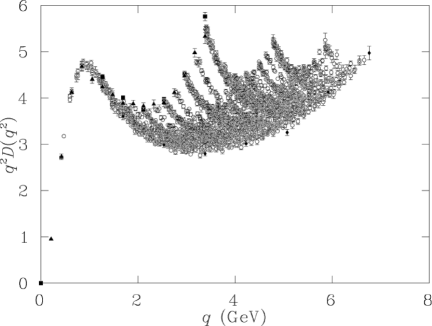
FIG. 1.: Uncorrected gluon propagator from lattice 1w ($\beta=5.70,16^{3}\times 32$, Wilson action), plotted as a function of $\hat{q}$. The dramatic “fanning” is caused by finite spacing errors which quickly destroy the signal at large momenta.

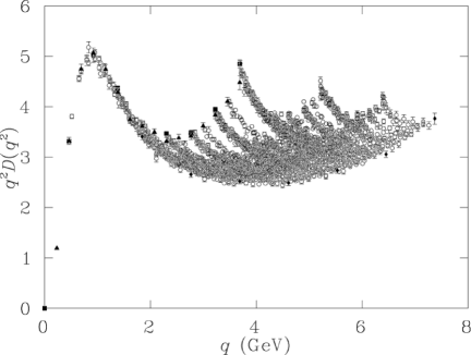
FIG. 2.: Uncorrected gluon propagator from lattice 1i ($\beta=4.38,16^{3}\times 32$, improved action), plotted as a function of $\hat{q}$. Lattice artifacts are reduced by the improved action, but are still large.

The most obvious way to deal with this noise is to apply an ultraviolet cut, considering only momenta out to half of the Brillouin zone. For each of the four Cartesian directions,

$$\hat{q}\leq\frac{\pi}{2a}.$$ (26)

We refer to this as the “half-cut” and in Fig. 3 and Fig. 4 we see that this removes the worst of the artifacts. The two propagators, show plausible asymptotic behaviors, but there are still clear signs of lattice artifacts and we have lost a lot of data in the ultraviolet. While neither of these shortcomings is a significant problem for studies of the infrared, we will show that something as crude as the half-cut is not necessary and we can do much better at minimizing lattice artifacts.

FIG. 3.: Uncorrected gluon propagator from lattice 1w ($\beta=5.70,16^{3}\times 32$, Wilson action), plotted as a function of $\hat{q}$ with the momentum “half-cut” applied.

FIG. 4.: Uncorrected gluon propagator from lattice 1i ($\beta=4.38,16^{3}\times 32$, improved action), plotted as a function of $\hat{q}$ with the momentum “half-cut” applied. The improved propagator has different normalization to the Wilson case due to a difference in the $Z_{3}$ renormalization constant.

We have already argued the case for applying a tree-level correction through the use of the alternative momentum variables derived from the tree-level behavior of the actions. The effect of doing this is seen in Fig. 5 and Fig. 6, where the Wilson propagator has been plotted as a function of $q^{W}$ ($q^{W}D(q^{W})$ vs. $q^{W}$) and the improved propagator as a function of $q^{I}$ ($q^{I}D(q^{I})$ vs. $q^{I}$) for all momenta of the Brillouin zone. Comparing these to Figs. 1 and 2, we see an excellent restoration of rotational symmetry all the way to the edge of the Brillouin zone. This is especially true of the improved action case in Fig. 6. The propagators also appear to be approaching their asymptotic, perturbative values. Later, momentum cuts will be applied to the data to further eliminate lattice artifacts, but for the moment it is interesting to keep all data, as they provide insight into the behavior of lattice simulations.

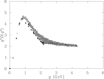
FIG. 5.: Uncut gluon propagator from lattice 1w ($\beta=5.70,16^{3}\times 32$, Wilson action), plotted as a function of $q^{W}$ for all momenta. The tree-level correction has greatly reduced discretization errors from those seen in Fig. 1.

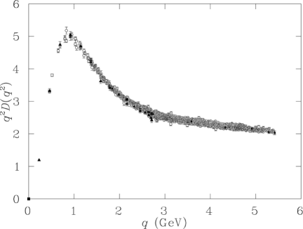
FIG. 6.: Uncut gluon propagator from lattice 1i ($\beta=4.38,16^{3}\times 32$, improved action), plotted as a function of $q^{I}$ for all momenta. The combination of improved action and tree-level correction has produced a remarkably clean signal over the entire range of accessible momenta. This figure should be compared with Fig. 2, and with Fig. 5 for the Wilson action at a similar lattice spacing.

Both Figs. 5 and 6 are consistent with the study of Ref. [17], but the discrepancy between diagonal and Cartesian points in Fig. 5 is a clear sign of rotational symmetry breaking in the unimproved case. With the Wilson action, the quality of the data is suffering from the coarseness of the lattice. As we might hope, the improved propagator in Fig. 6 shows excellent agreement between diagonal and Cartesian points, and the data is generally less spread. The propagator from the improved action has better rotational symmetry at the same lattice spacing. Less easy to understand is the slight suppression of the temporal points (triangles) in the Wilson case, Fig. 5. The time axis of this lattice (as with all the lattices considered here) is twice as long as the other three axes, so different values for the points along the long axis would normally be interpreted as a finite volume effect, yet there is no sign of it in the improved case (which has approximately the same physical volume). There is a difference between the improved and unimproved cases in the amplitudes of the propagators, but this is accounted for by renormalization and will be discussed below.

Out of curiosity the gluon propagator from lattice 1i has also been examined as a function of $q^{W}$, which we have already argued to be inappropriate. Not surprisingly, this leads to a “propagator” that suffers badly from lattice artifacts. We have not included a figure here, but the resulting propagator droops strongly in the ultraviolet. This is clearly a poor choice of momentum variable for this action as expected on the basis of our tree-level correction. For best results at finite lattice spacing, the correct momentum variable is determined by the appropriate tree-level behavior, which in turn is defined by the choice of action and gluon field definition. For the rest of this report it shall be implicit that when discussing quantities from the Wilson action, $q^{W}$ is used, and $q^{I}$ is used with the improved action.

FIG. 7.: Gluon propagator from lattice 5 at $\beta=4.10$, which has spacing $a\simeq 0.27\text{ fm}$ on $12^{3}\times 24$. This has the same physical volume as lattice 3 of Fig. 9. The propagator is shown for all momenta (no data cuts) after tree-level correction.

FIG. 8.: Gluon propagator from lattice 2, the smaller lattice at $\beta=3.92$ which has spacing $a\simeq 0.35\text{ fm}$ on a $10^{3}\times 20$ lattice. Finite volume errors are just detectable as indicated by momenta along the time axis (filled triangles) falling below the rest of the data. Tree-level correction has been used, but no data cuts have been applied.

FIG. 9.: Gluon propagator from lattice 3 at $\beta=3.75$, which has spacing $a\simeq 0.41\text{ fm}$ on $8^{3}\times 16$. The propagator is shown for all momenta (no data cuts) after tree-level correction. This propagator is consistent with that obtained on much finer lattices.

C Lattice Spacing Dependence

At this point it is interesting to explore the effect of making the lattice coarser. Figures 7, 8 and 9 show the uncut, tree-level corrected propagator on progressively coarser lattices ($a=$ 0.27, 0.35 and 0.41 fm respectively). Consider the most extreme case, shown in Fig. 9. This very coarse lattice has spacing $a=0.41\text{ fm}$, which is more than twice as coarse as the previous lattices. Any sign of a perturbative tail has been lost, as the UV cutoff has been lowered, but the infrared behavior remains. There is no sign of any qualitative change, which appears to indicate that even on such a coarse lattice we are not losing information vital to the infrared physics of the gluon propagator.

This gives us great confidence in the use of improved actions on coarse lattices for the probing of nonperturbative physics. This is the motivation for creating lattice 4 at $a=0.35$ on a very large volume. Fig 10, which shows the results from this large lattice, shows no signs of significant finite volume artifacts when compared with Fig. 8 which has the same lattice spacing, but a smaller volume.

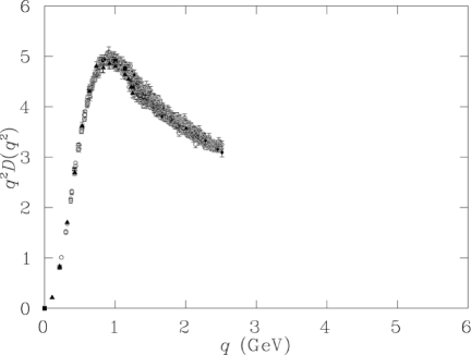
FIG. 10.: Gluon propagator from lattice 4, the larger lattice at $\beta=3.92$, which has spacing $a\simeq 0.35\text{ fm}$ on a $16^{3}\times 32$ lattice providing the largest physical volume of any in this study. Tree-level correction has been used, but no data cuts have been applied.

D Data Cuts

Having identified possible lattice artifacts, cuts may be applied to clean up the data, making it easier to draw conclusions about continuum physics. Data at large momenta will of course be most susceptible to finite lattice spacing errors. We choose to prefer data from momentum points near the four-diagonal, as this evenly samples all Cartesian directions, i.e., for a given momentum squared ($q^{2}$) it has the smallest values of each of the Cartesian components $q_{\mu}$. This should minimize finite lattice spacing artifacts.

We calculate the distance $\Delta\hat{q}$ of a momentum vector $\hat{q}$ from the diagonal using

$$\Delta\hat{q}=|\hat{q}|\sin\theta_{\hat{q}},$$ (27)

where the angle $\theta_{\hat{q}}$ is given by

$$\cos\theta_{\hat{q}}=\frac{\hat{q}\cdot\hat{n}}{|\hat{q}|},$$ (28)

and $\hat{n}=\frac{1}{2}(1,1,1,1)$ is the unit vector along the diagonal. In this way we ignore data points that are potentially most affected by hypercubic artifacts. We call this cut the cylinder cut [17]. From this point on, we exclude points greater than two spatial momentum units from the four-diagonal. Furthermore, the point at zero four-momentum has been cut from all the following plots of $q^{2}D(q)$. On any finite lattice, $D(0)$ must be finite, hence $q^{2}D(q)=0$ for $q=0$. This point is therefore trivial when plotting $q^{2}D(q)$. When the scalar function, $D(q)$, itself is considered we can make a study of $D(0)$ by considering it on lattices of differing volumes and then making an infinite volume extrapolation. We will perform this extrapolation below.

E Action Dependence

Once again we compare the gluon propagator generated with the Wilson action to that generated with the improved action after tree-level correction, this time applying the cylinder cut. To make the comparison in Fig. 11, we note that there is of course a small difference in normalization. This is the difference in the $Z_{3}$ renormalization between the Wilson and improved propagators. As the relative renormalization is $q^{2}$ independent, the unimproved propagator has been multiplied by a relative renormalization of 1.09 to make direct comparison possible. This factor is deduced by adjusting the vertical scales of the two data sets until they agreed. Apart from the superior performance of the improved propagator, which has already been discussed, the two actions produce the same result.

We push our results further by comparing the improved $\beta=4.38$ propagator with that from lattice 6 (Wilson action), which is finer ($a=0.1\text{ fm}$), has more points ($32^{3}\times 64$) and is a little larger. Both data sets are cylinder cut, and each is tree-level corrected according to its action. The relative renormalization has been determined to be $Z_{3}(\text{improved})/Z_{3}(\text{Wilson})=1.08$. It can be seen from Fig. 12 that not only are the two propagators consistent, but that the ultraviolet performance of lattice 1i is remarkable. The propagator from Ref. [17] had the momentum half-cut applied, whereas our improved propagator with lattice spacing $a=0.17\text{ fm}$ is shown for the entire Brillouin zone. We have calculated the propagator over the same range of momenta as Ref. [17], despite using a much coarser lattice.

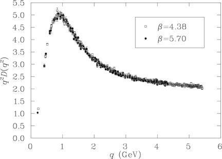
FIG. 11.: Comparison of the gluon propagator from lattices 1w at $\beta=5.70$ and 1i at $\beta=4.38$. Data has been cylinder cut and tree-level correction has been applied. We have determined $Z_{3}(\text{improved})/Z_{3}(\text{Wilson})=1.09$ by matching the vertical scales of the data.

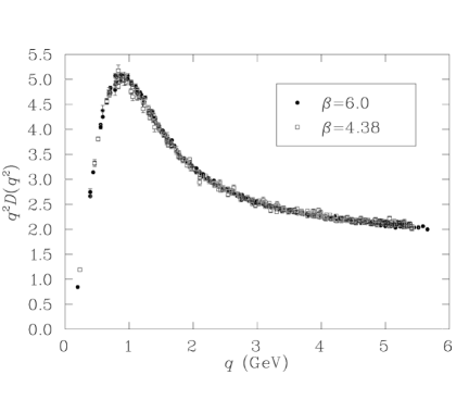
FIG. 12.: Comparison of the gluon propagator from the finest improved lattice (lattice 1i, $\beta=4.38$) and the finest Wilson lattice (lattice 6, $\beta=6.0$). Data has been cylinder cut and the appropriate tree-level corrections have been applied. The data from lattice 6 is half-cut whereas lattice 1i displays the full Brillouin zone. We have determined $Z_{3}(\text{improved})/Z_{3}(\text{Wilson})=1.08$ by matching the vertical scales of the data.

F Scaling Analysis

Next, we consider the propagator on the coarser lattices. Fig. 13 shows the propagator from lattices 1i, 2, 3 and 5. Examining Figures 11 and 13 we see that the Wilson $\beta=5.7$ and improved $\beta=4.10$ and $\beta=4.38$ results all agree well, which suggests that these are “fine enough” lattices. We see that the $\beta=3.75$ and $\beta=3.92$ propagators do not quite line up with the others, but instead the UV tail rises slightly as the lattice becomes coarser. This is an indication of a loss of scaling. The lattices at $\beta=3.92$ and $\beta=3.75$ having $a=0.35$ and 0.41 fm respectively are too coarse for the tree-level correction to completely correct the entire Brillouin zone, which is not surprising. We have placed extraordinary demands on our simulations by examining them near the cutoff. The conclusion is that such coarse lattices should be half-cut. Nevertheless, the propagators all agree in the infrared. Now that we have an understanding of the dependence of lattice propagator on the lattice spacing, we can study the effect of the finite volume.

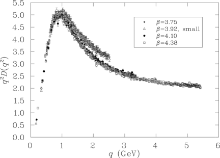
FIG. 13.: Comparison of the gluon propagator from lattices 1i ($\beta=4.38$), 2 ($\beta=3.92$, small), 3 ($\beta=3.75$), and 5 ($\beta=4.10$), which have a variety of lattice spacings. Data has been cylinder cut and tree-level correction has been applied. Data from the two finest improved lattices (0.17 and 0.27 fm) are consistent. A clear violation of scaling is seen in the coarsest two lattices (0.35 and 0.41 fm), where the spacing is too coarse for tree-level correction to completely restore the full Brillouin zone behavior.

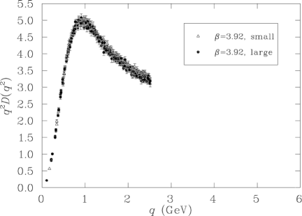
FIG. 14.: Comparison of the gluon propagator from lattices 2 and 4, which have the same lattice spacing ($a=0.35\text{ fm}$), but different lattice volumes. Notice that one lies directly over the other, despite having very different volumes. Data has been cylinder cut and tree-level correction has been applied.

G Volume Dependence

Results from lattices 2 and 4 have already been reported in Ref. [10] and are presented again here for completeness and ease of comparison. They have same lattice spacing, but different numbers of lattice points, and hence different physical volumes. The gluon propagator has been calculated on each lattice, and the results compared in Fig. 14. The two propagators are consistent in this figure, despite the fact that one lattice has sides 60% longer in all four directions. This shows that finite volume effects are small compared to the statistical errors. The turn over seen in the gluon propagator in lattice studies is certainly not a finite volume effect. Note that $5.65^{3}\times 11.30\text{ fm}^{4}$ is a very large volume by the standards of present day lattice studies, and gives us an unprecedented look at the behavior of QCD in the deep infrared.

FIG. 15.: Comparison of the gluon propagator generated with an improved action on five different lattices. We find good agreement down to $q\simeq 500$ MeV. At the lowest accessible momenta the data points drop monotonically with increasing volume, but the lowest point (on the largest lattice) shows signs of having converged to its infinite volume value. For comparison with perturbation theory, a plot of the continuum, tree-level gluon propagator (i.e., $1/q^{2}$ appropriately scaled) has been included.

FIG. 16.: Comparison of the lattice gluon propagator with that obtained from perturbation theory, in the ultraviolet to intermediate regime. The continuum expressions are tree-level (i.e., $1/q^{2}$ appropriately scaled) and the three-loop expression used in Ref. [2].

Fig. 15 shows the cylinder-cut data for the scalar function $D(q^{2})$ for each of the improved lattices. This plot provides a dramatic demonstration of lattice artifacts. In this way of plotting our results, the five lattices appear in very good agreement in the ultraviolet and through intermediate momenta. When plotted in this way, we can see that below $\sim 500\text{ MeV}$ the propagators do begin to differ due to finite volume effects. As the volume increases, the low momenta data points drop, until we can see the infrared flatten off. The grouping of points around 400 MeV suggest that we have, for the two largest lattices, results indicative of the infinite volume limit. At $\sim 250\text{ MeV}$, the results for the two largest lattices (both $\beta=3.92$) are consistent, and in particular the fact that the small difference between them is produced by such a large difference in volume gives us confidence in the results. For comparison, the tree-level, perturbative expression $D(q^{2})=1/q^{2}$ is also shown, suitably normalized.

It is interesting to note that the disagreement in the propagators above 1 GeV or so revealed in Fig. 13 is hidden by the scale of the vertical axis in Fig. 15. Multiplication of the propagator by $q^{2}$ is required to amplify this region and critically examine the extent to which lattice spacing artifacts are removed by ${\cal O}(a^{2})$ improvement terms. A failure to do this could lead to incorrect conclusions being drawn on the effectiveness of improvement in the gluon propagator. Thus it is always best to plot $q^{2}D(q^{2})$ versus $q^{2}$, when the hypercubic artifacts are of interest.

H Asymptotic Behavior

For further comparison with perturbation theory, we have chosen to show the gluon propagator from 1.5 to 5.5 GeV, in Fig. 16. In this window, the transition from perturbative to nonperturbative physics can be clearly seen. As well as the lattice gluon propagator and the tree-level, continuum propagator, we show a perturbative, three-loop calculation [22]. We used parameters obtained from Ref. [2], where at the renormalization point, $\mu=5.48$ GeV, the strong coupling constant was found to be $\alpha(\mu)=0.255$. That was a quenched calculation, so this number should not be compared directly with experiment. The data agree very well with three-loop perturbation theory down to $q\simeq 2.5$ GeV. Below 2 GeV we see that three-loop perturbation theory begins to fail.

I Propagator at Zero Four-Momentum

Values for the gluon propagator at zero four-momentum are shown in Table II for each of the lattices created in this investigation. Statistical errors are given in parentheses. The renormalization condition of Eq. (24) is enforced at the renormalization point $\mu=4.0$ GeV, which sets the scale for $D(q^{2})$. We see that as the volume of the lattice increases, $D(0)$ becomes smaller. In Fig. 17 we plot the infrared behavior of the renormalized gluon propagator for five lattices and we include the points calculated at zero momentum in this plot. We see that the the infrared behavior is quite smooth and reasonably consistent for our two largest volume lattices ($\beta=3.92$, small and large). Fig. 18 illustrates the data with a linear fit in the inverse volume according to

$$D(0)=c{1\over V}+D_{\infty}(0)$$ (29)

We find a reasonable fit with parameter values $c=245(22)\ {\rm fm}^{4}\,{\rm GeV}^{-2}$ and $D_{\infty}(0)=7.95(13)$ GeV^-2, where $D_{\infty}(0)$ is the infinite volume limit of the zero-momentum gluon propagator. Fig. 18 strongly supports the hypothesis that the gluon propagator is finite in the infrared. It is also clear that the results of our largest physical volume lattice are very close to the infinite volume limit.

Lattice	Dimensions	$\beta$	D(0)	D(0) ($\text{GeV}^{-2}$)	Volume ($\text{fm}^{4}$)
1i	$16^{3}\times 32$	4.38	32.0 (8)	10.4 (2)	97.2
1w	$16^{3}\times 32$	5.70	24.0 (5)	10.0 (2)	135
5	$12^{3}\times 24$	4.10	10.6 (3)	9.0 (2)	220
3	$8^{3}\times 16$	3.75	4.3 (1)	8.9 (2)	237
2	$10^{3}\times 20$	3.92	5.7 (1)	8.6 (2)	300
4	$16^{3}\times 32$	3.92	5.4 (1)	8.2 (2)	2038

TABLE II.: The value of gluon propagator at zero four-momentum for each of the lattices created in this investigation, in order of increasing volume. The raw (dimensionless) and physical values are given. In obtaining the physical values we have set the renormalization condition $D(\mu^{2})=1/\mu^{2}$ at $\mu=4.0$ GeV. An estimate of the uncertainty in the last figure is given in parentheses.

FIG. 17.: The renormalized gluon propagator is shown in the infrared region, including the points at zero four-momentum, from five lattices.

FIG. 18.: Values for the gluon propagator at zero four-momentum, $D(0)$, plotted as a function of the inverse lattice volume. The solid line represents a linear fit to the lattice results. The fit indicates the largest volume results are very close to the infinite volume limit and $D(0)=7.95(13)$ GeV^-2 in the infinite volume limit.

Note that a complete systematic extrapolation to the infinite volume limit remains to be carried out in the future. Ideally, one performs a number of calculations at fixed volume and various lattice spacings and then performs a continuum limit extrapolation for that fixed volume. This continuum limit extrapolation would be done for each of a variety of lattice volumes and then finally an infinite volume extrapolation performed on those results. This procedure corresponds to the axiomatic field theory prescription of taking the continuum limit before the infinite volume limit. Given this caution, the finite precision of this study, and the fact that the linear ansatz above may be incorrect, we can not completely exclude the possibility that the deep infrared (i.e., below $\sim$ 350 MeV) behavior of $D(q^{2})$ may very slowly decrease toward zero as the infinite volume limit is taken.

It is interesting to compare our results with a recent calculation of the gluon propagator in Laplacian gauge [23], which is expected to be free of gauge ambiguity. In that gauge, the propagator takes its perturbative, Landau-gauge value in the asymptotic region and is also infrared finite. The Laplacian gauge propagator is seen to have a behavior similar to that seen here.

V Conclusions

The gluon propagator has been calculated on a set of lattices with an ${\cal O}(a^{2})$ mean-field improved action, in ${\cal O}(a^{2})$ mean-field improved Landau gauge. Tree-level correction has been shown to reduce rotational symmetry breaking and dramatically improve the ultraviolet behavior of the propagator.

For $\beta\geq 4.10$ ($a\leq 0.27$ fm) the tree-level corrected improved propagator displays scaling over the entire Brillouin zone. At $\beta=4.38$ ($a=0.166$ fm), the gluon propagator has excellent behavior for the entire range of available momenta in the Brillouin zone, reproducing the anticipated UV behavior of perturbation theory to three-loops.

The infrared behavior of the gluon propagator is robust even with a lattice spacing of 0.41 fm. Calculation on a lattice with a large volume indicates that finite volume effects are small. In particular, the turn over observed in previous studies of the Landau gauge gluon propagator is not a finite volume artifact. We conclude that the propagator is almost certainly infrared finite, in agreement with earlier studies. A significant volume dependence is revealed only at the smallest non-trivial momenta. An extrapolation of $D(0)$ via a linear ansatz inversely proportional to the physical lattice volume provides a reasonable fit. Moreover, results from our largest volume lattice reside very close to the infinite volume limit. We have probed the approach to the infinite volume limit by first determining a range of $\beta$ in which the propagator scales for $q<0.7$ GeV on similar finite volumes. Physically large volumes are accessed by decreasing $\beta$ within the scaling range on large lattices. A more complete study of the infinite volume limit should be undertaken in the near future.

The tree-level corrected results from our $\beta=3.92$ ($a=0.353$ fm) $16^{3}\times 32$ lattice with a physical volume of $5.65^{3}\times 11.30=2038$ fm⁴ may be regarded as an excellent estimate of the infinite volume, continuum limit Landau-gauge gluon propagator for $q<0.7$ GeV. The tree-level corrected results from our $\beta=4.38$, ($a=0.166$ fm) results presented here are an excellent estimate of the infinite volume, continuum limit of the Landau-gauge gluon propagator for $q>0.7$ GeV. We have seen that these two sets of data smoothly match in the intermediate regime ($q\sim 0.7$ GeV) and are entirely consistent with each other in this region. The possible effects of lattice Gribov copies remains a very interesting question and we plan to extend this study to Laplacian gauge and other related gauge-fixing schemes in the near future.

REFERENCES

- [1] Jeffrey E. Mandula, The Gluon Propagator, hep-lat/9907020; C. D. Roberts and A. G. Williams, Prog. Part. Nucl. Phys. 33, 477 (1994).
- [2] D. Becirevic et al., Phys. Rev. D 60, 094509 (1999); ibid. D 61, 114508 (2000).
- [3] G. Peter Lepage, Redesigning Lattice QCD, hep-lat/9607076.
- [4] See for example, F.X. Lee & D.B. Leinweber, Phys. Rev. D 59, 074504 (1999), and references therein.
- [5] Kazuyuki Kanaya, hep-lat/9804006.
- [6] G.P. Lepage & P.B. Mackenzie, Phys. Rev. D 48, 2250 (1993).
- [7] K. Symanzik, Nucl. Phys. B 226, 187 (1983) ibid. pp. 205ff.
- [8] P. Weisz, Nucl. Phys. B 212, 1 (1983); P. Weisz & R. Wohlert, Nucl. Phys. B 236, 397 (1984); Erratum–ibid. B 247, 544 (1984).
- [9] M. Lüscher and P. Weisz, Commun. Math. Phys. 97, 59 (1985).
- [10] F.D.R. Bonnet, P.O. Bowman, D.B. Leinweber & A.G. Williams, Phys. Rev. D 62, 051501 (2000).
- [11] P.O. Bowman, A. Hotan, D.B. Leinweber & A.G. Williams, in preparation.
- [12] N. Cabibbo & E. Marinari, Phys. Lett. B 119, 387 (1982).
- [13] F. D. Bonnet, D. B. Leinweber and A. G. Williams, General algorithm for improved lattice actions on parallel computing architectures, to be published in J. Comp. Phys., hep-lat/0001017.
- [14] A. Cucchieri, Phys. Rev. D 60, 034508 (1999).
- [15] A. Cucchieri & T. Mendes, Phys. Rev. D 57, 3822 (1998).
- [16] F.D.R. Bonnet, P.O. Bowman, D.B. Leinweber, D.G. Richards & A.G. Williams, Aust. J. Phys. 52, 939 (1999); Nucl. Phys. B (Proc. Suppl.) 83-84, 905 (2000).
- [17] D.B. Leinweber, J-I. Skullerud, A.G. Williams & C. Parrinello, Phys. Rev. D 58, 031501 (1998); ibid. D 60, 094507 (1999); Erratum–ibid. D 61, 079901 (2000).
- [18] P. Marenzoni, G. Martinelli, N. Stella, Nucl. Phys. B 455, 339 (1995).
- [19] J.P. Ma, Mod. Phys. Lett. A 15, 229 (2000).
- [20] J-I. Skullerud & A.G. Williams, Phys. Rev. D 63, 054508 (2001); D.B. Leinweber, J-I. Skullerud & A.G. Williams, hep-lat/0102013.
- [21] F.D.R. Bonnet, D.B. Leinweber, A.G. Williams & J. Zanotti, in preparation.
- [22] Philippe Boucaud, private communication.
- [23] C. Alexandrou, Ph. de Forcrand & E. Follana, hep-lat/0008012.