Abstract

We propose new techniques for the numerical implementation of the overlap-Dirac operator, which exploit the physical properties of the underlying theory to avoid nested algorithms. We test these procedures in the two-dimensional Schwinger model and the results are very promising. These techniques can be directly applied to QCD simulations. We also present a detailed computation of the spectrum and the chiral properties of the Schwinger model in the overlap lattice formulation.

1 Introduction

The last few years witnessed a major breakthrough in the lattice regularization of Fermi fields. The closely related domain wall [1] and overlap [2, 3] formulations of lattice fermions provide a definition of a lattice Dirac operator $D$ which avoids the doubling problem and preserves the relevant symmetries of the continuum theory, most notably chiral symmetry in the limit of vanishing fermion mass. Unfortunately, this welcome development has come at a price: the numerical calculation of the matrix elements of the propagator $D^{-1}$ and the inclusion of ${\rm Det}(D)$ in the measure entail a substantially increased computational burden, which severely constrains the maximum lattice size for viable simulations. Many efforts have recently been devoted to finding more efficient ways to perform these computational tasks [4]. The problem has generally been approached from a numerical analysis point of view, looking for approximations that allows one to use sparse matrix techniques, although $D$ itself is not sparse. In this article we would like to advocate and explore a different approach, where the approximation is based on the physics and proceeds through a projection over a subspace, which has a substantially reduced number of degrees freedom but still captures the relevant long range properties. Our approximation consists in taking the matrix elements of the Wilson Dirac operator in a subspace consisting of the long range modes which we expect to dominate the low energy properties of the theory and in constructing the overlap Dirac operator numerically, but without further approximations, in this subspace. In the complement, the Dirac operator is approximated by its free form. The projection over long range modes is done via a Fourier transform after gauge fixing. We also studied a gauge invariant method of projection. We will compare the results obtained with our approximation in a simplified model with those of an exact calculation, finding satisfactory agreement. It is our hope that the approximation may offer a new way to implement the overlap formulation in four-dimensional QCD.

We will focus on the overlap Dirac operator and we will apply our approximation procedure to the two-dimensional Schwinger model. We use the overlap formulation because it provides an exact framework for the new lattice fermions. The domain wall formulation becomes exact in the limit of infinite extent in the extra dimension, in which case it becomes equivalent to the overlap formulation up to corrections that vanish with the lattice spacing. With finite extent in the extra dimension, the domain wall formulation can be viewed as a numerical approximation to the exact result. Since one of our goals is to compare the results of our approximation to exact results, the overlap formulation is better indicated. We study the Schwinger model because the system is simple enough that we will be able to calculate $D^{-1}$ and ${\rm Det}(D)$ exactly as well as in our proposed scheme of approximation. The results of the exact calculations are, we believe, interesting per se, because they are more extensive than what, to the best of our knowledge, has been done up to now and validate in an impressive manner the advantages of the new formulation of lattice fermions.

The plan of this paper is as follows. In the next section we will briefly review known properties of the Schwinger model in the continuum and in the lattice overlap formulation. In Section 3 we will present the results of a numerical simulation where propagator and determinant of the overlap Dirac operator are calculated exactly. In Section 4 we will introduce the proposed scheme of approximation, which is based on the projection over a reduced number of degrees of freedom. We will compare the results obtained with this approximation with those of the exact calculation. In Section 5 we will describe an approximation to the determinant of $D$, based on a coarsening of the lattice and compare results obtained with the full and approximated determinants. In the last section we will present a few words of conclusion.

2 The Schwinger Model and the Overlap Formulation

We consider the Schwinger Model in (two-dimensional) Euclidean space-time and we allow for $N_{f}$ degenerate flavors. The model is defined by the action

$$S=\int d^{2}x\left[\frac{1}{4}F_{\mu\nu}F_{\mu\nu}+\sum_{i=1,N_{f}}\bar{\psi}_{i}(D_{\mu}\gamma_{\mu}+m)\psi_{i}\right]$$ (1)

where $\psi_{i}$, $\bar{\psi}_{i}$ are two components spinors, $A_{\mu}$ is the $U(1)$ gauge potential, $D_{\mu}=\partial_{\mu}+igA_{\mu}$ and $F_{\mu\nu}=\partial_{\mu}A_{\nu}-\partial_{\nu}A_{\mu}$. We will use the following two-dimensional representation of $\gamma$-matrices

$$\gamma_{1}=\sigma_{1}\;,\qquad\gamma_{2}=\sigma_{2}\;,\qquad\gamma_{5}=-i\gamma_{1}\gamma_{2}=\sigma_{3}$$ (2)

where $\sigma_{i}$ are the Pauli matrices.

The topological charge of a classical gauge configurations is

$$Q(A)\equiv\frac{g}{4\pi}\int d^{2}x\,\epsilon_{\mu\nu}F_{\mu\nu}(x)$$ (3)

while the index of the Dirac operator is given by the difference between the numbers of positive ($n_{+}$) and negative ($n_{-}$) chirality zero modes

$$\mbox{index}(A)\equiv n_{-}-n_{+}$$ (4)

The Atiyah-Singer theorem states that

$$Q(A)=\mbox{index}(A)\equiv n_{-}-n_{+}$$ (5)

Moreover in two dimensions the vanishing theorem ensures that [5]

$$n_{+}\neq 0 \rightarrow n_{-}=0$$

$$n_{-}\neq 0 \rightarrow n_{+}=0$$ (6)

At the quantum level the Schwinger model does not require infinite renormalization: $g$ and $m$ are finite bare parameters. In the massless limit the model can can be solved exactly [6]. In the following we will analyze the systems with $N_{f}\leq 2$. Information for generic $N_{f}$ can be found in [7].

2.1 The Schwinger model with $N_{f}=1$.

The classical theory has a vector $U(1)_{V}$ symmetry and a softly broken axial symmetry $U(1)_{A}$, which at the quantum level is also broken by the anomaly. The Ward Identities (WI) for the corresponding quantum theory are

$$\partial_{\mu}V_{\mu}=0\;,\qquad\partial_{\mu}A_{\mu}=\frac{g}{2\pi}\epsilon_{\mu\nu}F_{\mu\nu}+2mP$$ (7)

where the Axial and Vector currents are defined as

$$V_{\mu}(x)=\bar{\psi}(x)\gamma_{\mu}\psi(x)\;,\qquad A_{\mu}(x)=\bar{\psi}(x)\gamma_{\mu}\gamma_{5}\psi(x)=-i\epsilon_{\mu\nu}V_{\nu}\;,$$ (8)

and the scalar and pseudoscalar densities are

$$S(x)=\bar{\psi}(x)\psi(x)\;,\qquad\qquad P(x)=\bar{\psi}(x)\gamma_{5}\psi(x)\;.$$ (9)

It is a peculiar property of the two-dimensional space-time that the vector and the axial currents are not independent of each other.

In the massless case a free fermion field factorizes and the Schwinger photon acquires a mass due to the anomaly. The photon’s field $\Phi$ is

$$V_{\mu}=\frac{1}{\sqrt{\pi}}\epsilon_{\mu\nu}\partial_{\nu}\Phi$$ (10)

and the vector current correlator

$$\langle V_{\mu}(x)V_{\nu}(y)\rangle_{0}$$ (11)

is the same as for a free massive propagator with mass $(\mu_{0}/g)^{2}=1/\pi$. The chiral condensate is

$$\frac{\langle\bar{\psi}\psi\rangle_{0}}{g}=-\frac{e^{\gamma}}{2\pi^{3/2}}$$ (12)

where $\gamma=0.577216\dots$ is Euler’s constant. Note that the formation of the fermion condensate, as in one-flavor QCD, does not imply spontaneous symmetry breaking; the $U(1)$ chiral symmetry is already broken by the anomaly.

For small masses the corrections to the massless results can be obtained using chiral perturbation theory [8, 9] and the Schwinger mass at the first order is given by

$$\Big{(}\frac{\mu_{1}}{g}\Big{)}^{2}=\frac{1}{\pi}-4\pi\frac{\langle\bar{\psi}\psi\rangle_{0}}{g}\Big{(}\frac{m}{g}\Big{)}$$ (13)

2.2 The Schwinger model with $N_{f}=2$.

In the model with two degenerate massive flavors, the classical theory has a $U(1)_{V}\times SU(2)_{V}$ vector symmetry, an axial $SU(2)_{A}$ symmetry softly broken by the mass term and a $U(1)_{A}$ symmetry broken by the quantum corrections. The Ward identities corresponding to the axial and vector $U(1)$ symmetries are analogous to the previous case. The Ward identities associated to the non-singlet axial and vector currents are given by

$$\partial_{\mu}V^{a}_{\mu}=0$$ (14)

and

$$\partial_{\mu}A^{a}_{\mu}=2mP^{a}$$ (15)

where

$$\qquad V^{a}_{\mu}=\bar{\psi}\frac{\lambda^{a}}{2}\gamma_{\mu}\psi\;,\qquad A^{a}_{\mu}=\bar{\psi}\frac{\lambda^{a}}{2}\gamma_{\mu}\gamma_{5}\psi\;,\qquad P^{a}=\bar{\psi}\frac{\lambda^{a}}{2}\gamma_{5}\psi$$ (16)

and $\lambda^{a}\equiv\sigma^{a}$ are the generators of the $SU(2)$ in flavor space. The non-singlet axial Ward identity (15) will be one of the key ingredients to test the properties of the overlap regularization.

In the massless limit, there are one massive singlet particle ($\eta$) with mass $(\mu_{\eta}/g)^{2}=N_{f}/\pi$ and a triplet of massless particles ($\pi$). Analogously to the $N_{f}=1$ model, the correlation functions of the vector currents are the same as for free particles. Unlike QCD, the chiral condensate $\langle\bar{\psi}\psi\rangle_{0}=0$. In fact a non-zero fermion condensate would break spontaneously the $SU_{A}(2)$ chiral symmetry of the model. But spontaneous symmetry breaking is not possible in two dimensions [10]. In this case also, the corrections to the massless results can be obtained by a semi-classical analysis [11] and the masses for triplet and singlet are

$$\frac{M_{\pi}}{g} = c\left(\frac{m}{g}\right)^{2/3}\qquad c=e^{2\gamma/3}\frac{2^{5/6}}{\pi^{1/6}}=2.163\dots$$ (17)

$$\left(\frac{M_{\eta}}{g}\right)^{2} = \frac{2}{\pi}+\left(\frac{M_{\pi}}{g}\right)^{2}$$

2.3 The Dirac Operator in the Overlap Formulation.

In the lattice regularization of the Schwinger model, the fermionic fields are defined over the sites of a square lattice, with lattice spacing $a$, and the gauge potentials are replaced with $U(1)$ link variables $U_{\mu}(x)$ defined over the oriented links of the lattice. The Euclidean lattice action is given by

$$S_{L}=\beta\sum_{x,\mu<\nu}\left[1-\mbox{Re}\,U_{\mu\nu}(x)\right]+a^{2}\sum_{i=1}^{N_{f}}\sum_{x,y}\bar{\psi}_{i}(x)\left[\,(1-\frac{am}{2})D(x,y)+m\right]\,\psi_{i}(y)$$ (18)

where $\beta=1/(ag)^{2}$, $g$ being the bare coupling constant,

$$U_{\mu\nu}(x)=U_{\mu}(x)U_{\nu}(x+a\hat{\mu})U^{{\dagger}}_{\mu}(x+a\hat{\nu})U^{{\dagger}}_{\nu}(x)$$ (19)

$\hat{\mu}$ being a unit vector in direction $\mu$, and $D$ is the lattice Dirac operator in the overlap formulation, as introduced by Neuberger. Occasionally we will also refer to $D$ as the Neuberger-Dirac operator. $D$ is constructed as follows. One starts from the massless Wilson-Dirac operator

$$D_{W}=\frac{1}{2}\gamma_{\mu}(\nabla_{\mu}+\nabla^{*}_{\mu})-\frac{1}{2}a\nabla^{*}_{\mu}\nabla_{\mu}$$ (20)

where $\nabla_{\mu}$ and $\nabla^{*}_{\mu}$ are the forward and backward lattice derivative, i.e.

$$\nabla_{\mu}\psi(x) = \frac{1}{a}[U_{\mu}(x)\psi(x+a\hat{\mu})-\psi(x)]$$

$$\nabla_{\mu}^{*}\psi(x) = \frac{1}{a}\left[\psi(x)-U^{\dagger}_{\mu}(x-a\hat{\mu})\psi(x-a\hat{\mu})\right]$$ (21)

One performs a polar decomposition of $D_{w}-1/a$, expressing this operator in terms of a unitary operator $V$ and its modulus

$$D_{W}-\frac{1}{a}=V\left[\left(D_{W}^{\dagger}-\frac{1}{a}\right)\left(D_{W}-\frac{1}{a}\right)\right]^{\frac{1}{2}}$$ (22)

From Eq. 22 it follows that $V$ is given by

$$V=\left(D_{W}-\frac{1}{a}\right)\left[\left(D_{W}^{\dagger}-\frac{1}{a}\right)\left(D_{W}-\frac{1}{a}\right)\right]^{-\frac{1}{2}}$$ (23)

Finally, the Neuberger-Dirac operator for a fermion of bare mass $m$ is given by

$$D=\left(\frac{1}{a}-\frac{m}{2}\right)\left(1+V\right)+m$$ (24)

The Neuberger-Dirac operator satisfies the $\gamma_{5}$-Hermiticity condition

$$D^{\dagger}=\gamma_{5}D\gamma_{5}$$ (25)

Moreover, for $m=0$ it satisfies the Ginsparg-Wilson (GW) relation [13]

$$\gamma_{5}D^{-1}+D^{-1}\gamma_{5}=a\gamma_{5}$$ (26)

which implies that the fermion action (18) at finite lattice spacing is invariant under the following continuous symmetry [14]

$$\delta\psi=\gamma_{5}(1-aD)\psi,\qquad\delta\bar{\psi}=\bar{\psi}\gamma_{5}$$ (27)

This can be interpreted as the lattice form of chiral symmetry. The corresponding flavor non-singlet chiral transformations are defined including a flavor group generator in Eq. (27).

The $\gamma_{5}$-Hermiticity condition (25) and the GW relation (26) imply further algebraic relations which can turn out to be useful in numerical simulations [15]. In particular

$$D+D^{\dagger}=aDD^{\dagger}=aD^{\dagger}D$$ (28)

hence $D$ and $D^{\dagger}$ commute, i.e. $D$ is normal and therefore the eigenvector are mutually orthonormal.

It is important to stress that locality, the absence of doubler modes and the correct classical continuum limit are not guaranteed by the GWR in Eq. (26). Indeed, there exist lattice fermion actions which satisfy the GWR but which do not meet the above requirements [16]. The Neuberger operator satisfies all the above requirements and is local in the weak coupling regime, as shown in Ref. [17].

The geometrical definition of the topological charge on the lattice is

$$Q=\frac{1}{2\pi}\mbox{Im}\sum_{x}\log(U_{12})$$ (29)

The flavor-singlet chiral transformations in Eq. (27) leads to chiral Ward identities analogous to the ones in Eq. (7) and the anomaly term arises from the non-invariance of the fermion integral measure [14]. The non-singlet chiral transformations analogous to Eq. (27) and the locality of the Neuberger-Dirac operator imply axial Ward identities analogous to Eq. (15) and therefore the quark mass renormalizes only multiplicatively, i.e. the critical bare mass is zero, the corresponding conserved axial and vector currents do not need renormalization and there is no mixing between 4-fermion operators in different chiral representations [18, 19]. Finally, the chiral condensate requires a subtraction and is defined as

$$\chi=-\langle\bar{\psi}(1-\frac{a}{2}D)\psi\rangle$$ (30)

3 Numerical Results from an Exact Calculation

In order to test our method of approximation and, at the same time, to increase the body of information on the lattice Schwinger model, we performed an extensive simulation with the exact calculation of Neuberger-Dirac operator and its inverse. For previous numerical work on the Schwinger model in the overlap regularization see [20]-[24]. We considered the Schwinger model with $\beta=6$ on a square lattice with $N_{x}=N_{y}=24$. On a lattice of this size, the discretized Dirac operator is a complex matrix of dimension $1152\times 1152$, for which we could use full matrix algebra subroutines without excessive burden on the resources available to us (the whole calculation used approximately 20,000 processor hours on the Boston University SGI/Cray Origin 2000 supercomputer). Having settled on the lattice size, we selected $\beta=6$ on the basis of previous results which indicated that, for most of the fermion masses we were planning to consider, the lattice would span at least a few correlation lengths. We generated 500 configurations of the gauge variables $U_{\mu}(x)$ distributed according to the pure gauge measure

$$S_{G}=\beta\sum_{x,\mu<\nu}\left[1-\mbox{Re}\,U_{\mu\nu}(x)\right]$$ (31)

(see also Eq. 19). These were obtained by a standard Metropolis Monte Carlo simulation, with 10000 upgrades of the whole lattice between subsequent configurations. With the pure gauge measure the plaquettes are essentially uncorrelated, apart from the constraint coming from the periodic boundary conditions, so the procedure we followed should be amply adequate to produce independent configurations. For calculations with one and two flavors of dynamical fermions, we incorporated the determinant of the lattice Dirac operator in the averages giving the observables. While with large variations of the determinant this way of proceeding would lead to an unacceptable variance, in the present calculation we found the range of values taken by ${\rm Det}(D)$ to be sufficiently limited to warrant our averaging procedure (see Fig. 16 in Section 5.) This is of course due to the rather small size of our system. With larger systems one should incorporate the determinant (or a suitable approximation to it) in the measure used for the simulation.

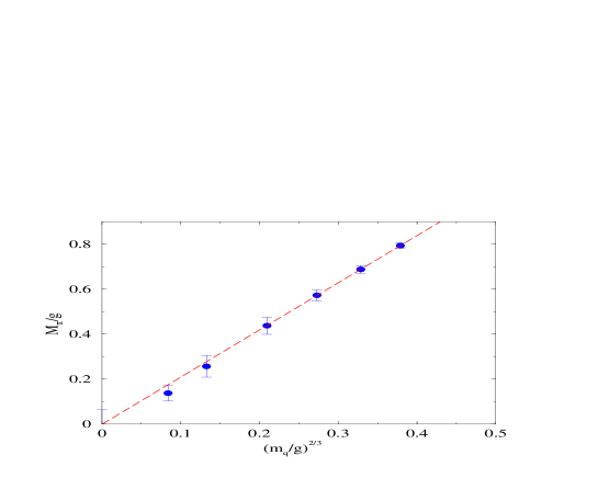
Figure 1: $M_{\pi}/g$ vs. $(m/g)^{2/3}$ for the full operator for $N_{f}=2$. The dashed line represents the fit as in Eq. 35 of the four highest masses.

For each configuration, we performed a singular value decomposition

$$D_{W}-\frac{1}{a}=U\Lambda\tilde{U}$$ (32)

where $U,\tilde{U}$ are unitary matrices and $\Lambda$ is diagonal, real and non-negative. The operator $V$ in Eq. 22 is given by

$$V=U\tilde{U}$$ (33)

We proceeded then to the diagonalization of $V$, calculating all its eigenvalues and eigenvectors. From these, it is clearly straightforward to calculate both the determinant of the Neuberger-Dirac operator $D$ as well as its associated propagator $D^{-1}$ for any value of the fermion mass $m$. The full diagonalization of $V$ is computationally more demanding then the direct calculation of $D^{-1}$, which typically gives also ${\rm Det}(D)$ as a by-product, but we were interested in the actual spectrum of $V$ for comparison with the approximations that will be discussed later. From the fermion propagators we calculated the meson propagators projected over zero momentum. We focused on the vector correlators

$$\langle\sum_{x,y,y^{\prime}}\bar{\psi}(x,y)\gamma_{2}\psi(x,y)\bar{\psi}(x+t,y^{\prime})\gamma_{2}\psi(x+t,y^{\prime})\rangle$$ (34)

because they are saturated by a single particle contribution in the massless limit. Practitioners of lattice calculations will certainly appreciate the value of being able to sum over all source locations, as opposed to having to deal with selected columns of the meson propagators. Of course we added to the averages the correlators obtained from the interchange of $x$ and $y$ in Eq. 34 for a further gain in statistics.

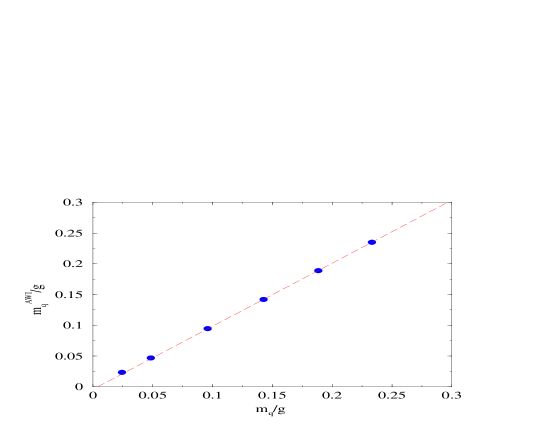
Figure 2: $m^{AWI}/g$ vs. $m/g$ for the full operator for $N_{f}=2$.

From fits to the meson correlators we extracted the meson masses in a standard manner. Figures 1, 2, 3, 4 reproduce our results for the meson masses as functions of the fermion mass. The values we obtained for the masses are also reported in the tables included in Sect. 4. The errors have been evaluated with the jackknife method. Figure 1 illustrates the behavior of the isotriplet mass $M_{\pi}$ in the model with two flavors. This mass is expected to vanish for $m=0$ and chiral perturbation theory predicts an $m^{2/3}$ dependence on $m$ (see Eq. 17). The dashed line in the figure shows the results for the fit

$$M_{\pi}/g=A+B(m/g)^{2/3}$$ (35)

for the four heaviest masses, which satisfy the condition $N_{x}M_{\pi}>4$ and therefore are less likely to be affected by finite volume effects. This fit gives $A=-0.001(65)$ and $B=2.10(14)$. We also performed the fit

$$M_{\pi}/g=C(m/g)^{\gamma}$$ (36)

which gives $C=2.10(17)$ and $\gamma=0.67(7)$. These results confirm in an impressive manner the chiral properties of the Neuberger operator and the mass dependence expected by analytical calculations [11, 12].

Equally gratifying is the comparison of the value of the fermion mass $m$ in the Lagrangian with the value $m^{AWI}$ that can be extracted, up to discretization effects, from the lattice analog of the axial Ward identity in Eq. 15. As shown in Fig. 2, the intercept and the slope of the linear fit through the four heaviest masses are compatible with zero and one respectively.

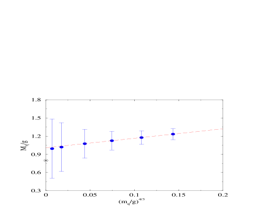
Figure 3: $M_{\eta}/g$ vs. $(m/g)^{4/3}$ for the full operator for $N_{f}=2$.

In Fig. 3 we illustrate the behavior of the singlet mass $M_{\eta}$ versus $m^{4/3}$, always for $N_{f}=2$. The singlet meson propagator is given by the difference of the connected and disconnected terms in the correlator and, because of the cancellations, the errors are larger than in the triplet case. The numerical results are, however, consistent with the theoretical prediction of Eq. 17.

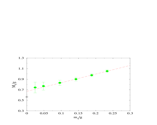
Figure 4: $M_{\eta}/g$ vs. $(m/g)$ for the full operator for $N_{f}=1$.

Finally, in Fig. 4 we display the singlet mass in the single flavor case. The errors are smaller than in the two flavor case because of the different relative weight of the connected and disconnected contributions. Again we find reasonable agreement between numerical results and the theoretical prediction.

4 Approximation of the Neuberger-Dirac Operator

Anybody who has ever seen a plot of the spectrum of eigenvalues of the Wilson-Dirac operator cannot but be left with the impression that there is a huge redundancy of states. The projection over a translated unitary circle done by the Neuberger-Dirac operator avoids the problem of mode doubling, but preserves the overall count of states. Yet, it would appear that the physical properties of the system should be determined by the eigenstates of $D$ with eigenvalues in the neighborhood of $\lambda=m$ (i.e. the eigenstates of $V$ with eigenvalue $\lambda_{V}$ closest to $-1$, cfr. Eqs. 23, 24), since these are the states with a smooth long range behavior, expected to go over the physical states of the continuum in the limit $a\to 0$. This suggests that it should be possible to reconstruct the physical observables from these states alone. The way in which such states contribute to physical observables has been studied in the literature [21]. Here we would like to make the point that the overlap formulation is particularly well suited for the implementation of the above approximation, since the unitarity of $V$ provides, in some sense, a checkpoint on the approximation itself. Of course, one must be careful in attempting any approximation based on neglecting the short-wavelength part of the spectrum, even if the corresponding states are largely lattice artifacts, since one knows that in quantum field theory the infrared and ultraviolet components of the spectrum are subtly related. Thus, the chiral eigenstates with $\lambda_{V}=-1$ (“zero modes”), which $V$ exhibits in presence of a gauge field with non-trivial topology, find their counterpart in states with opposite chirality at $\lambda_{V}=1$. Here too, however, the special features of the overlap formulation come to the rescue, since, as we will show, both the presence of zero modes and the correspondence between $\lambda_{V}=-1$ and $\lambda_{V}=1$ eigenstates of opposite chirality can be preserved by the projection over a subset of physical states. In this section we will illustrate such a projection by comparing the approximate results for the observables with those of the exact calculation.

One possible scheme of approximation which is computationally very convenient consists in performing a projection over states of low momentum in Fourier space, after gauge fixing to a smooth gauge field configuration. In a smooth gauge, because of the suppression of short-wavelength fluctuations due to asymptotic freedom, one expects the structure of the Wilson operator come more and more diagonal in momentum space for increasing momenta. This notion is schematically illustrated in Fig. 5 and also underlies the technique of Fourier acceleration for the calculation of quark propagators [25]. Accordingly, we implemented the following approximation.

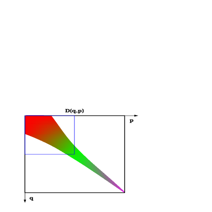
Figure 5: Structure of the Wilson operator in momentum space and in a smooth gauge.

We fixed the gauge on all configurations to the Landau gauge by demanding that the function

$$G=\sum_{x,\mu}{\rm Re}[U_{\mu}(x)]$$ (37)

be maximal. A relaxation procedure produces several local maxima (Gribov copies). Among all these configurations, we selected the one that produced the absolute maximum for $G$, subject to the further constraint that for all $x$ and $\mu$ ${\rm Re}U_{\mu}(x)\geq 0.5$. Some care must be exerted with the configurations that have non-vanishing topological number $Q$. These configurations cannot be brought to a uniformly smooth gauge. To discuss them further it is convenient to introduce the notation

$$U_{\mu}(x)=e^{\imath\theta_{\mu}(x)}$$ (38)

$$U_{\mu\nu}(x)=e^{\imath\theta_{\mu\nu}(x)}$$ (39)

Then, with $Q\neq 0$ there must be one or more plaquettes where

$$\theta_{\mu\nu}(x)=\theta_{\mu}(x)+\theta_{\nu}(x+a\hat{\mu})-\theta_{\mu}(x+a\hat{\nu})-\theta_{\nu}(x)+2m\pi$$ (40)

with $m$ a non-zero integer. This implies that for such plaquettes

$${\rm Abs}[\theta_{\mu}(x)+\theta_{\nu}(x+a\hat{\mu})-\theta_{\mu}(x+a\hat{\nu})-\theta_{\nu}(x)]\geq\pi$$ (41)

and thus the corresponding gauge variables cannot be all close to unity. We will call these plaquettes the “hot spots” of the gauge configuration. Their location is gauge dependent but, as long as $Q\neq 0$, they cannot be eliminated. For the configurations $C_{Q}$ with $Q\neq 0$ we fixed the gauge as follows. First we created a configuration $C^{\prime}$ with the same value of $Q$ by superimposing gauge field configurations in the Landau gauge with uniform $U_{\mu\nu}(x)$ and $Q=1$. We placed the hot spots of this configurations in the locations where the action of the original field configuration was smaller, using a weighting procedure that minimized the overlap of hot spots. Then we brought to the Landau gauge the gauge field configuration $C^{\prime\prime}$ obtained subtracting $C^{\prime}$ from $C_{Q}$. Finally we superimposed $C^{\prime}$ to the gauge transformed $C^{\prime\prime}$. The resulting configuration is gauge equivalent to the original $C_{Q}$, is approximatly in the Landau gauge and is “reasonably smooth”, the latter statement being justified a posteriori by the application of our approximation. Clearly the procedure described above relies heavily on the Abelian nature of the gauge field and will have to be generalized to handle non-Abelian systems.

After gauge fixing, we project the lattice Wilson-Dirac operator over the subspace $\cal F$ of Fourier space spanned by the eigenvectors with lowest momenta. For the results we present in this paper, the projection was done over the subspace defined by

$$(p_{x}a)^{2}+(p_{y}a)^{2}\leq(p_{c}a)^{2}$$ (42)

where the cut-off momentum $p_{c}$ was chosen so that the total number of momenta included in the projection equals 145, i.e. a fraction $z\approx 1/4$ of the total number of momenta. (We could not choose $p_{c}$ in such a way as to project over exactly one fourth of the space, since the number of momenta satisfying Eq. 42 is always odd.) Accordingly, the dimensionality of $\cal F$ is 290, out of a total dimensionality of the fermion field equal to 1152 ($24\times 24$ lattice sites $\times 2$ spin degrees of freedom). This corresponds to an effective reduction of a factor of two for each dimension of the lattice. As a matter of fact, we experimented with even smaller values of $z$ and found that, with $Q=0$, $z$ can be chosen substantially smaller than $1/4$ without spoiling the good quality of the approximation. For configurations with a non-trivial topology the infrared properties of the Wilson operator are still well reproduced on the subspace. However the real doubler modes of the truncated Wilson operator are shifted towards the infrared region and, as they pass the projection point, the association between topology and chirality is lost.

The approximation to the Neuberger-Dirac operator is obtained following the construction of Eqs. 22 and 23, where $D_{W}$ and $V$ are replaced by their projections over $\cal F$: $\tilde{D}_{W}$ and $\tilde{V}$ (see also [26]). If we denote by $D_{W}^{(0)}$ the projection of the free Dirac operator over the complement of $\cal F$ and by $V^{(0)}$ the corresponding unitary factor in its polar expansion, we finally take

$$V_{approx}=\tilde{V}\oplus V^{(0)}$$ (43)

as our approximation to $V$. More specifically, given any fermionic vector $\psi$, we project it over $\cal F$ and its complement: $\psi=\psi_{F}+\psi_{\bar{F}}$. $V_{approx}\psi$ is then given by $\tilde{V}\psi_{F}+V^{(0)}_{\bar{F}}$.The approximate form of the Neuberger-Dirac operator follows from Eq. 24.

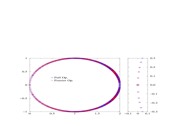
Figure 6: Comparison of spectra on a configuration with $Q=1$.

The first check on the approximation is that it should reproduce well the spectrum of long range modes, i.e. those with $V$ eigenvalues in the neighborhood of -1. In particular, configurations with $Q\neq 0$ should have $|Q|$ eigenvectors with $V$ eigenvalue exactly equal to -1. This turned out to be the case. With the chosen cut-off $p_{c}$ (See Eq. 42) the approximation consistently gives satisfactory results for the spectrum of long range modes. We display in Fig. 6 the spectrum of eigenvalues of the exact $1+V$ (x symbols - blue) and the approximate $1+\tilde{V}$ (plus symbols - red) for a configuration with $Q=1$. The matching in the physical part of the spectrum, close to $0$, is excellent (see the blow-up at the right of the figure). Also, as we anticipated above, the approximation preserves the presence of a zero mode, which is a chiral eigenstate. It is worthwhile to notice that $\tilde{V}$ is constructed from a projected Wilson operator $\tilde{D}_{W}$ which has the same $\gamma_{5}$ transformation properties as the original Wilson operator. Thus $\tilde{V}$ will have the same $\gamma_{5}$ transformation properties as $V$ and, in particular, its eigenvectors with eigenvalue $-1$ will be matched by a corresponding number of eigenvectors with eigenvalue $1$. Since $V^{(0)}$ has no eigenvectors with eigenvalues $\pm 1$, this carries over to the $V_{approx}$.

Figure 7: Chiral condensate from the exact calculation.

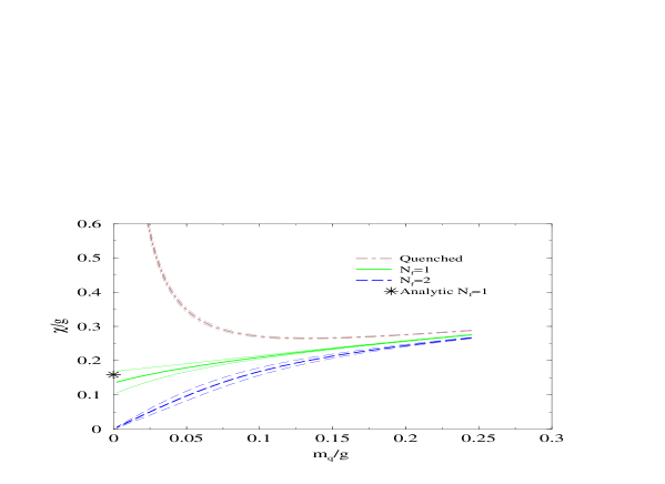
Figure 8: Chiral condensate with the Fourier approximation.

Closely related to the spectrum is the value of the chiral condensate. It is instructive to reexpress the condensate of Eq. 30 in terms of the eigenvalues of $V$. With $a=1$ we find

$$\chi=-\frac{1}{N_{f}}\langle\bar{\psi}(1-\frac{1}{2}D)\psi\rangle=\frac{1}{N_{x}N_{y}}\frac{1}{1-m/2}\frac{\langle{\rm Det}(D)^{N_{f}}{\rm Tr}\Big{[}D^{-1}-\frac{1}{2}\Big{]}\rangle_{U}}{\langle{\rm Det}(D)^{N_{f}}\rangle_{U}}$$ (44)

(We use the subscript $U$ in the r.h.s. of this equation as a reminder that the averages are quenched averages over the gauge field. See also the discussion following Eq. 31.) Using Eq. 24 we get

$$\chi=\frac{1}{N_{x}N_{y}}\frac{\langle{\rm Det}(D)^{N_{f}}\Big{[}\frac{|Q|}{m}+\frac{m}{2}\sum_{j}\frac{1-\cos\phi_{j}}{(1+m^{2}/4)+(1-m^{2}/4)\cos\phi_{j}}\Big{]}\rangle_{U}}{\langle{\rm Det}(D)^{N_{f}}\rangle_{U}}$$ (45)

where we separated in the sum the $|Q|$ pairs of eigenvalues equal to -1 and 1 from the others, which occur in pairs of complex conjugate values $\exp(\pm\imath\phi_{j})$.

Figure 7 reproduces the result of the exact calculation, Fig. 8 the result obtained by inserting in Eq. 45 the eigenvalues obtained with the Fourier approximation. The two sets of results are indistinguishable (we did not plot them on the same graph, because one set of lines would have covered the other). The crosses on the two figures show the analytic result for $m=0$, $N_{f}=1$.

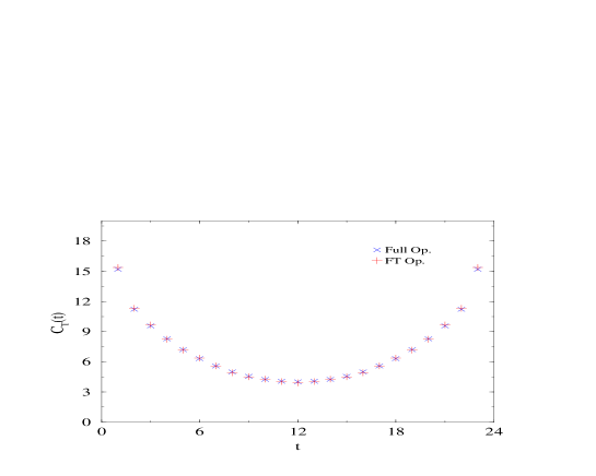
Figure 9: Results for $\gamma_{2}$-triplet propagator on a configuration with $Q=0$.

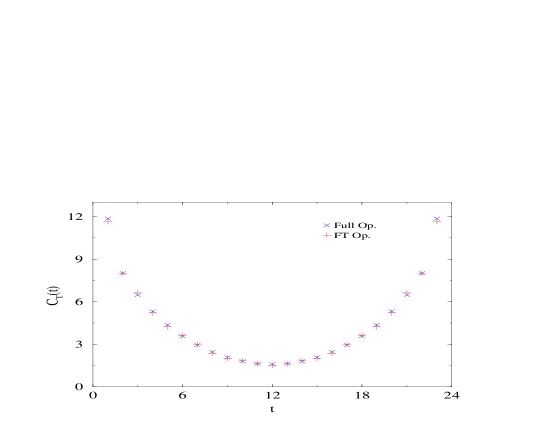
Figure 10: Results for $\gamma_{2}$-triplet propagator on a configuration with $Q=-1$.

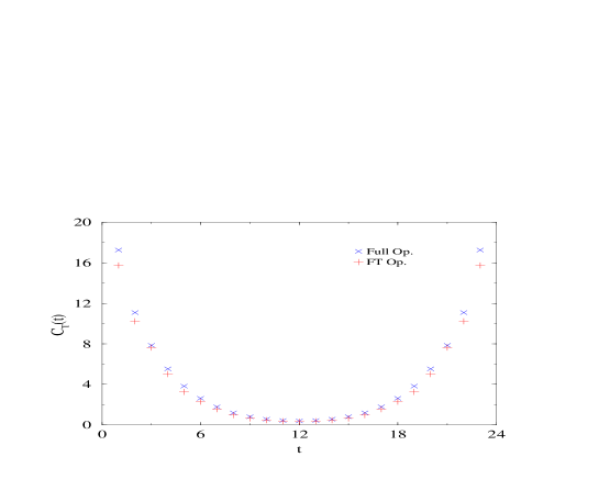
Figure 11: Results for $\gamma_{2}$-triplet propagator on a configuration with $Q=4$.

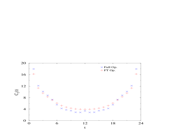
Figure 12: Disconnected part of the $\gamma_{2}$-singlet propagator on a configuration with $Q=0$.

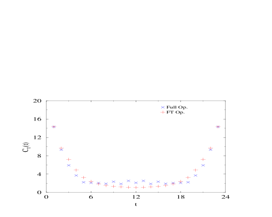
Figure 13: Disconnected part of the $\gamma_{2}$-singlet propagator on a configuration with $Q=-1$.

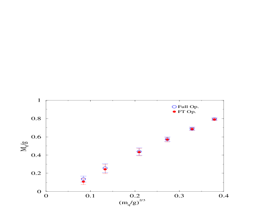
Figure 14: $M_{\pi}/g$ vs. $(m/g)^{2/3}$ for the full operator and the gauge-fixing approximation for $N_{f}=2$.

Another test of the approximation is obtained by comparing configuration by configuration the propagators for fermion bilinears. Our approximation gives quite satisfactory results for the connected Green’s functions. We reproduce in Figs. 9, 10 and 11 the propagator of the $\gamma_{2}$-triplet bilinear in three randomly chosen configurations with $Q=0,-1$ and $4$, respectively. We see that propagators obtained from the approximation to the Neuberger-Dirac operator compare quite well with those obtained from the exact operator, even with $Q=4$.

Our results for the disconnected Green’s functions are not conclusive. We reproduce in Figs. 12, 13 the disconnected parts of the propagator in the same configurations as used for Figs. 9, 10. The approximate propagators are smoother than the exact ones, which can be understood as an effect of the truncation over the short wavelength modes, but not incompatible in an average sense. Of more concern is that we found the fluctuations of the approximate disconnected propagators to be substantially larger than in the exact calculation. The large fluctuations of the disconnected components in the exact calculation already makes the error in the singlet masses rather big. The even larger fluctuations of the disconnected components in the approximate calculation prevented us from obtaining in this case a meaningful result for the singlet masses.

We reproduce in the tables all the masses which we were able to calculate. We see that whenever we could get a mass value from the Fourier approximation, the result turned out in reasonably good agreement with the exact calculation. A fit to Eqs. 35 and 36 of the approximate calculation gives the following results for the parameters: $A=-0.005(65)$, $B=2.10(15)$, $C=2.10(17)$ and $\gamma=0.67(7)$ with excellent agreement with the results of the full calculation, presented immediately after Eqs. 35 and 36. A comparison between masses in the exact and approximate calculations is also presented in Fig. 14.

$\beta=6.0$, $V=24^{2}$
$m/g$	$m_{\pi}/g$	$m^{AWI}_{q}/g$
Full Operator
0	0.15(1)	-0.0026(2)
0.0244	0.393(13)	0.0234(1)
0.0485	0.442(10)	0.0472(2)
0.0960	0.553(8)	0.0949(3)
0.1427	0.661(6)	0.1420(4)
0.1884	0.761(6)	0.1884(4)
0.2333	0.857(5)	0.2343(5)
Fourier Approximation
0.0	0.14(1)	-0.0049(3)
0.0244	0.385(13)	0.0208(3)
0.0485	0.435(10)	0.0427(5)
0.0960	0.548(8)	0.0875(8)
0.1427	0.656(7)	0.1321(11)
0.1884	0.758(6)	0.1761(13)
0.2333	0.855(5)	0.2194(16)

Table 1: Masses for $N_{f}=0$.

$\beta=6.0$, $V=24^{2}$
$m/g$	$m_{\eta}/g$
Analytic
0	0.5642
Full Operator
0	0.67(6)
0.0244	0.74(10)
0.0485	0.77(8)
0.0960	0.83(5)
0.1427	0.90(4)
0.1884	0.98(3)
0.2333	1.05(3)
Multigrid Det.
0	0.68(6)
0.0244	0.75(10)
0.0485	0.78(7)
0.0960	0.84(5)
0.1427	0.91(4)
0.1884	0.98(3)
0.2333	1.06(3)

Table 2: Masses for $N_{f}=1$.

$\beta=6.0$, $V=24^{2}$
$m/g$	$m^{AWI}$	$m_{\pi}/g$	$m_{\eta}/g$
Analytic
0	0	0	0.7979
Full Operator
0.00	-0.004(2)	-0.001(65)	1.00(25)
0.0244	0.0233(2)	0.14(3)	1.0(5)
0.0485	0.0468(6)	0.26(5)	1.0(4)
0.0960	0.0945(13)	0.44(4)	1.1(2)
0.1427	0.1420(14)	0.57(3)	1.1(2)
0.1884	0.1890(13)	0.69(2)	1.2(1)
0.2333	0.2353(11)	0.79(1)	1.23(9)
Fourier Approximation
0.00	-0.002(2)	-0.005(66)	-
0.0244	0.018(1)	0.11(3)	-
0.0485	0.044(1)	0.24(5)	-
0.0960	0.092(1)	0.43(4)	-
0.1427	0.139(1)	0.57(3)	-
0.1884	0.184(1)	0.68(2)	-
0.2333	0.228(1)	0.79(1)	-
Multigrid Determinant
0.00	-0.004(1)	-0.002(40)	1.09(25)
0.0244	0.0234(1)	0.14(2)	1.1(4)
0.0485	0.0469(4)	0.26(3)	1.1(4)
0.0960	0.0946(9)	0.44(2)	1.1(2)
0.1427	0.1420(10)	0.57(2)	1.2(2)
0.1884	0.1889(9)	0.68(1)	1.2(1)
0.2333	0.2351(8)	0.79(1)	1.26(9)

Table 3: Masses for $N_{f}=2$.

In closing this section let us mention a different, gauge invariant scheme of approximation, which we also tried. We built the subspace $\cal F$ used for the projection of Eq. 43 out of the lowest eigenvectors of the negative of the covariant Laplacian, namely the operator (see Eq. 21)

$$-\Delta=-\sum_{\mu}\nabla_{\mu}\nabla^{*}_{\mu}$$ (46)

The lowest eigenmodes of $-\Delta$ are typically slowly varying, whereas the highest modes exhibit rapid variations from site to site. Thus the subspace $\cal F$ formed out of the lowest eigenvectors of $-\Delta$ is well suited to represent the physical excitations of the system. The construction of this subspace is gauge-invariant and, contrary to the approximation based on the Fourier transform, does not require any gauge fixing. Finding a sufficiently large number of eigenvectors of $-\Delta$ is however computationally expensive. An even more serious problem is that this approximation does not provide any simple way to define the projection of a “free operator” on the complement of $\cal F$: the form of the free Wilson operator is clearly gauge dependent. Thus, for lack of better alternatives, we replaced $V{(0)}$ in Eq. 43 with the identity operator, projecting all the remaining eigenvalues to $1$. As a consequence of this rather drastic projection, the propagators of the bilinears turned out to exhibit oscillations around the exact propagators, with much less satisfactory agreement than we found in the Fourier approximation. While these oscillations do not necessarily rule out the possibility of still obtaining good values for the masses through a suitable fitting procedure, the worst quality of the bilinear propagators together with the higher computational costs dissuaded us from pursuing this approximation further.

5 Coarse grid Approximation to the Determinant

In the previous section we explored the possibility to truncate the Neuberger operator to its long range components on a given gauge configuration. In the spirit of long range approximations, there is another possibility that can be explored, which is the coarse graining of the Dirac operator, as done in multigrid calculations [27].

Figure 15: Sketch of the blocking procedure. Original Links corresponding to a site in the coarse lattice are fixed to local Landau gauge. Links between them are averaged according to Eq. 48 to give links of the blocked lattice.

A preliminary step is the projection of the gauge field to a coarser lattice. Starting from an arbitrary gauge configuration on an $N\times N$ lattice, we apply a blocking procedure to arrive at a gauge configuration on a coarser $N/2\times N/2$ lattice designed in such a way that the coarser lattice should carry the long range features of the finer $N\times N$ lattice. The absence of additive mass renormalization then allows one to define a Neuberger operator on the coarser lattice, which is related to the Neuberger operator on the finer lattice without tuning of the bare mass and reproduces all its long range features. One could then in principle measure the Green’s functions on the coarser lattice. It would however be no trivial problem to interpolate them back to the finer lattice compensating for the errors introduced by coarsening. We therefore decided only to measure the determinant on the coarse lattice and compare it to the one on the fine lattice.

Figure 16: $\log{\rm Det}(D)$ on the blocked lattice versus $\log{\rm Det}(D)$ on the full lattice, for lightest mass, $m/g=0.0244$, on the full system.

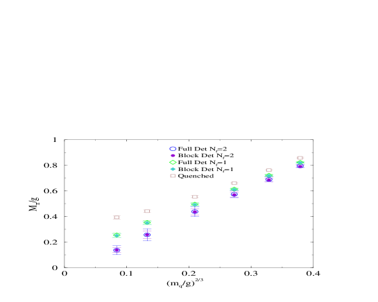
Figure 17: $M_{\pi}/g$ vs. $(m/g)^{2/3}$ for the full determinant and for the blocked one.

To block a gauge field $U_{\mu}(x,t)$ on an $N\times N$ lattice down to a gauge field $\bar{U}_{\mu}(\bar{x},\bar{t})$ on an $N/2\times N/2$ lattice we applied the following procedure:

• Divide the sites of the fine lattice into $N/2\times N/2$ blocks of $2^{2}$ sites. The center of each of these blocks will correspond to a site $(\bar{x},\bar{t})$ in the coarse lattice.

• Fix the gauge such that the links connecting sites within one block are as close as possible to unity, i.e.,

  $$\sum_{\bar{x},\bar{t}=0}^{N/2-1}\left(U_{\hat{x}}(2\bar{x},2\bar{t})+U_{\hat{t}}(2\bar{x},2\bar{t})+U_{\hat{x}}(2\bar{x},2\bar{t}+1)+U_{\hat{t}}(2\bar{x}+1,2\bar{t})\right)\rightarrow\mbox{max}$$ (47)

• Construct the link between two sites of the coarse lattice as close as possible to the links between the corresponding fine lattice blocks, i.e.,

  $$\left((U^{{\dagger}}_{\hat{t}}(2\bar{x},2\bar{t}+1)+U^{{\dagger}}_{\hat{t}}(2\bar{x}+1,2\bar{t}+1))\bar{U}_{\hat{t}}(\bar{x},\bar{t})\right) \rightarrow$$ maxand (48)

  $$\left((U^{{\dagger}}_{\hat{x}}(2\bar{x}+1,2\bar{t})+U^{{\dagger}}_{\hat{x}}(2\bar{x}+1,2\bar{t}+1))\bar{U}_{\hat{x}}(\bar{x},\bar{t})\right) \rightarrow$$ max

Figure 15 gives a picture of how the blocking is done.

As stated above, we calculated the fermion determinant on the blocked lattice and compared it to the determinant on the full lattice. As shown in Fig. 16, the blocked determinant follows the full determinant closely. Moreover the eigenvalues of $V$ exactly equal to $-1$ are always preserved by the blocking. Thus one would expect the effects of dynamical fermions to be well reproduced by an approximation where the blocked determinant is used instead of the full determinant.

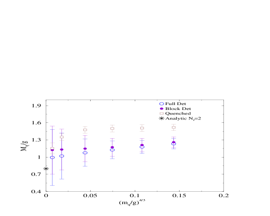
Figure 18: $M_{\eta}/g$ vs. $(m/g)^{4/3}$ with the full, blocked and quenched determinant for the full operator for $N_{f}=2$.

This is confirmed by results shown in Figs. 17 and 18. In Fig. 17 we reproduce the values of the isotriplet mass $M_{\pi}$ obtained by using either the full determinant or the blocked determinant in the calculation of the observables. We see that the results obtained with the blocked determinant are in very good agreement with those obtained with the full determinant. The physical results are those for $N_{f}=2$. We inserted in the figure also the results of a quenched calculation and of a calculation with $N_{f}=1$ in order to highlight the effects of the determinant. In particular, one sees that the data support a linear dependence of $M_{\pi}$ versus $(m_{q}/g)^{2/3}$ with $M_{\pi}$ vanishing in the chiral limit only when one has $2$ dynamical quark flavors, i.e. when one uses the square of the full determinant ${\rm Det}^{2}(D)$ as weight factor. (This observation is based on the data for the 4 rightmost points in the figure, which have $N_{x}M_{\pi}<4$ and thus are less likely to be affected by finite size effects – see also the fit in Fig. 1 and the discussion that follows.) This nontrivial result does not change however, when ${\rm Det}^{2}(D)$ is replaced by the square of the blocked determinant ${\rm Det}^{2}_{\rm block}(D)$.

We reproduce in Fig. 18 the results for the singlet mass $m_{\eta}$ for $N_{f}=2$. Once again we also include the results of a quenched calculation to show the effect of the determinant. In this case also unquenching with the blocked determinant is consistent with unquenching with the unblocked determinant. The results however are less impressive, since the observable contains disconnected propagators and is therefore very noisy.

6 Conclusions

We have explored, in the context of the overlap formulation of lattice fermions, a scheme of approximation which focuses on the physical properties of the system and takes advantage of the special features of the Neuberger-Dirac operator. Our method of approximation is based on the projection of the Wilson operator on a subspace of lower dimensionality, where the Neuberger-Dirac operator and its inverse are constructed by dense matrix techniques. We tested our approximation on the Schwinger model, finding satisfactory results. Of course, the main interest of any scheme of approximation for overlap fermions is in its applicability to four-dimensional QCD. The possibility of a successful extension of our method to this theory will depend on how much one can reduce the dimensionality of the space used for the projection with respect to the full space, while keeping a good approximation to the physical observables.

In the two-dimensional Schwinger model, the simplest implementation of these ideas has been able to reduce the dimensionality of the fermionic vector space by a factor of approximately 4. If this is an indication that one can achieve a reduction of a factor of two per space-time dimension, it would mean that in four dimensions the dimensionality of the fermionic space can be reduced by a factor of order 16. This may not be enough for QCD calculations on lattices of realistic size, but even larger reductions of dimensionality are not necessarily out of the question. In our experiment with the Schwinger model, we found that we could reduce the dimensionality of the subspace used for the projection by a factor ranging well above 4 (as much as 10 or more while still keeping a good approximation to physical observables) for the configurations with trivial topology. As mentioned in Section 4, for configurations with non-trivial topology the infrared properties of the Wilson operator are well captured even on small subspaces, but the Neuberger projection mixes then eigenvectors with different chiralities. This could however be more a shortcoming of the basis used for the projection, i.e. the Fourier basis, than of the method of approximation in itself.

Even if it turned out that the reduction of dimensionality one can achieve is not sufficient for a practical use of dense matrix techniques in the projection subspace, the approximation we have studied can still be of value. The Neuberger-Dirac operator and its inverse could be calculated within the subspace with sparse matrix numerical techniques similar to those currently in use for the whole space, with the advantage of having to deal with a substantially smaller system. Alternatively, the approximate eigenvectors obtained by the projection could be used for a preconditioning of the calculation of the propagators on the full space. This is a possibility which we have not explored in our work, mostly for limitations of time and resources, but which might be worth studying in a future investigation. It is likely, though, that incorporating in the computational techniques used for dealing with overlap fermions as much insight as possible on the properties of the physical excitations will pay handsome rewards, and we are currently investigating the application of our approximation method to four-dimensional lattice QCD.

References

-
[1]
D. B. Kaplan, Phys. Lett. B288 (1992) 342.
Y. Shamir, Nucl. Phys. B406 (1993) 90.
T. Blum et al., hep-lat/0007038. - [2] R. Narayanan and H. Neuberger, Nucl. Phys. B443 (1995) 305.
-
[3]
H. Neuberger,
Phys. Lett. B417 (1998) 141.
H. Neuberger, Phys. Lett. B427 (1998) 353. -
[4]
H. Neuberger, Phys. Rev. Lett. 81 (1998) 4060.
R. G. Edwards, U. M. Heller and R. Narayanan, Nucl. Phys. B540 (1999) 457.
A. Borici, Phys. Lett. B453 (1999) 46.
S. J. Dong, F. X. Lee, K. F. Liu and J. B. Zhang, Phys. Rev. Lett. 85 (2000) 5051.
T. DeGrand, Phys. Rev. D63 (2001) 034503. -
[5]
J. Kiskis,
Phys. Rev. D15 (1977) 2329.
N. K. Nielsen and B. Schroer, Nucl. Phys. B127 (1977) 493.
M. M. Ansourian, Phys. Lett. B70 (1977) 301. - [6] J. Schwinger, Phys. Rev. 128 (1962) 2425.
- [7] C. Gattringer and E. Seiler, Annals Phys. 233 (1994) 97.
-
[8]
S. Coleman, R. Jackiw and L. Susskind,
Annals Phys. 93 (1975) 267.
S. Coleman, Annals Phys. 101 (1976) 239. - [9] C. Adam, Annals Phys. 259 (1997) 1 and references therein.
-
[10]
N. D. Mermin, H. Wagner,
Phys. Rev. Lett. 17 (1966) 1133;
P. C. Hohenberg, Phys. Rev. 158 (1967) 383;
S. Coleman, Commun. Math. Phys. 31 (1973) 259. - [11] C. Gattringer, I. Hip and C. B. Lang, Phys. Lett. B466 (1999) 287.
- [12] A. V. Smilga, Phys. Rev. D55 (1997) 443.
- [13] P. H. Ginsparg and K. G. Wilson, Phys. Rev. D25 (1982) 2649.
- [14] M. Lüscher, Phys. Lett. B428 (1998) 342.
- [15] F. Niedermayer, Nucl. Phys. (Proc.Suppl.) 73 (1999) 105 and references therein.
- [16] T. Chiu, C. Wang and S. V. Zenkin, Phys. Lett. B438 (1998) 321.
- [17] P. Hernandez, K. Jansen and M. Lüscher, Nucl. Phys. B552 (1999) 363.
- [18] P. Hasenfratz, Nucl. Phys. B525 (1998) 401.
- [19] S. Capitani and L. Giusti, Phys. Rev. D62 (2000) 114506 and hep-lat/0011070.
- [20] R. Narayanan, H. Neuberger and P. Vranas, Phys. Lett. B353 (1995) 507 and Nucl. Phys. Proc. Suppl. 47 (1996) 596.
- [21] J. Kiskis and R. Narayanan, Phys. Rev. D62 (2000) 054501.
-
[22]
F. Farchioni, I. Hip and C.B. Lang,
Phys. Lett. B443 (1998) 214.
F. Farchioni, I. Hip, C.B. Lang and M. Wohlgenannt, Nucl. Phys. B549 (1999) 364. - [23] S. Chandrasekharan, Phys. Rev. D59 (1999) 094502.
- [24] W. Bietenholz, I. Hip, Nucl. Phys. B570 (2000) 423.
- [25] G. Katz, G. Batrouni, C. Davies, A. Kronfeld, P. Lepage, P. Rossi, B. Svetitsky and K. Wilson, Phys. Rev. D37 (1988) 1589.
- [26] L. Giusti, C. Hoelbling and C. Rebbi, Nucl. Phys. (Proc. Suppl.) 83-84, (2000) 896.
- [27] R. Brower, R. Edwards, C. Rebbi and E. Vicari, Nucl. Phys. B366 (1991) 689.