Lattice instanton action from 3D SU(2) Georgi-Glashow model

Abstract:

3D Georgi-Glashow model is studied on the lattice in the London limit in an infrared but an intermediate region before the screening appears. Abelian and instanton dominances are observed after abelian projections in a unitary gauge and roughly in the maximally abelian gauge. Using an inverse Monte-Carlo method, we determine an effective instanton action in both gauges. When we restrict ourselves to some regions of parameters $\beta$ and $\kappa$, we obtain an almost perfect instanton action, performing a block-spin transformation on the dual lattice. It takes a form of a Coulomb gas and reproduces fairly well the string tension obtained analytically by Polyakov. The almost perfect actions in both gauges look the same in the infrared region, which suggests gauge independence.

1 Introduction

It is very important to understand confinement mechanism of QCD. Wilson’s lattice formulation [1] shows that the confinement is a property of a non-Abelian gauge theory of strong interaction and there are a lot of numerical lattice calculations showing the confinement of color. But the mechanism of confinement is still not well understood.

One of approaches to the confinement problem is to search for relevant dynamical variables and to construct an effective theory in terms of these variables. In 1970’s, it was pointed out that the confinement of quarks may be explained as the dual Meissner effect due to condensation of monopoles [2, 3].

In (QCD)₄, ’t Hooft[4] proposed an idea of abelian projection. After a partial gauge fixing (called as abelian projection), SU(N) gauge theory can be reduced to an abelian U(1)^N-1 theory with $N-1$ different charges and magnetic charges. Namely, $N-1$ monopoles appear after the abelian projection. Quark confinement could be understood by the dual Meissner effect due to condensation of these monopoles. Actually there have been many numerical data supporting the above conjecture when one performs the abelian projection in the Maximally abelian (MA) gauge.

The first interesting findings are some phenomena called abelian dominance. Abelian Wilson loops composed of abelian link variables alone seem to reproduce essential features of quark confinement in the Maximally Abelian gauge [5].

The second is monopole dominance. It has been shown that monopoles alone are responsible for abelian quantities in the infrared region. Abelian Wilson loops and abelian Polyakov loops are written as a product of monopole and photon contributions. The monopoles which are defined by DeGrand and Toussaint[6] reproduce the confinement features [7].

Furthermore an effective lattice monopole action was derived by Shiba and Suzuki[8] in a simple case with two-point interactions alone. The work was extended to include 4 and 6 point interactions in [9] and [10].

There is another system having such a magnetic quantity naturally. It is the three-dimensional Georgi-Glashow model (GG)₃ where there exist a famous ’t Hooft-Polyakov instanton [11, 12] having a magnetic charge. Polyakov showed analytically [13] that the string tension of 3D Georgi-Glashow model has a finite value. He made a quasi-classical calculation using a dilute Coulomb gas approximation of ’t Hooft-Polyakov instantons. However justification of his method is not clear. If the quasi-classical assumption using the dilute instanton gas is true, abelian and instanton dominances should hold in the infrared region of three-dimensional Georgi-Glashow model. It is expected naturally that an effective abelian instanton action works well in the infrared region.

It is shown in [14] that Polyakov’s picture of the dilute Coulomb instanton gas is too simple to describe all infrared physics of (GG)₃. Actually, it can not explain the screening of doubly charged particle due to $W^{\pm}$ bosons. However, such a screening appears only for particles with even charge and also in the long infrared range of $O(2M_{W}/\sigma)$, where $M_{W}$ is a mass of the W boson and $\sigma$ is the string tension. Hence if we restricted ourselves to an infrared but an intermediate region before the screening appears, we may be allowed to adopt such a picture as Polyakov’s one.

It is just the purpose of this study to test the Polyakov’s assumptions and to check calculations done by him quantitatively formulating the theory on the lattice and restricting ourselves to the intermediate region before the screening appears. Our method is Monte-Carlo numerical simulations without ad-hoc assumptions. In Section 2, we briefly review the Polyakov’s work in 1977[13]. We calculate the total energy of ’t Hooft-Polyakov instanton in the London limit. In Section 3, we show the method of our numerical study. We derive a lattice instanton action in 3D Georgi-Glashow model using an inverse Monte-Carlo method. We then perform a block-spin transformation of DeGrand-Toussaint instantons. These discussions are almost similar to those in 4D pure QCD in MA gauge fixing[8]. In Section 4, we show our numerical results of the lattice monopole action in 3D Georgi-Glashow model. Then we calculate the string tension derived by Polyakov using the parameters determined in our numerical simulations. Section 5 is devoted to concluding remarks.

2 Confinement mechanism in 3D Georgi-Glashow model

We review briefly the ’t Hooft-Polyakov instanton and confinement mechanism due to the instantons as discussed by Polyakov in Ref[13].

2.1 Georgi-Glashow model and ’t Hooft-Polyakov instanton

The three-dimensional Georgi-Glashow model is given by

$$S=\int{\rm d}^{3}x\left\{\frac{1}{4}F_{\mu\nu}^{a}F_{\mu\nu}^{a}+\frac{1}{2}{\cal D}_{\mu}\phi^{a}{\cal D}_{\mu}\phi^{a}+\frac{\lambda}{4}(\phi^{a}\phi^{a}-v^{2})^{2}\right\},$$ (1)

where

$$F^{a}_{\mu\nu}=\partial_{\mu}A^{a}_{\nu}-\partial_{\nu}A^{a}_{\mu}+g\epsilon^{abc}A^{b}_{\mu}A^{c}_{\nu},$$ (2)

$${\cal D}_{\mu}\phi^{a}=\partial_{\mu}\phi^{a}+g\epsilon^{abc}A^{b}_{\mu}\phi^{c}.$$ (3)

It is a SU(2) Yang Mills theory with an adjoint Higgs field. It has a phase with spontaneously broken symmetry (SU(2) $\rightarrow$ U(1)) and the gauge field becomes massive because of the Higgs mechanism. The gauge boson mass is given at the tree level by

$$m_{W}\simeq gv.$$ (4)

In the case of three space-time dimensions, the theory has an instanton solution —— ’t Hooft-Polyakov instanton. One instanton solution takes the form [11]

$$\phi^{a} = \frac{r^{a}}{gr^{2}}H(gvr),$$ (5)

$$A^{a}_{\mu} = \frac{1}{g}\varepsilon_{a\mu b}\frac{r^{b}}{r^{2}}[1-K(gvr)],$$ (6)

where $H$ and $K$ are dimensionless functions determined by the equations of motion. They satisfy

$$\left.\begin{array}[]{l}K(gvr)\longrightarrow 0\\ H(gvr)\longrightarrow gvr\end{array}\right\}r\rightarrow\infty.$$ (7)

For the ansatz given in Eqs.(5) and (6), the energy of the one-instanton system is given by

$$S=\frac{4\pi v}{g}\int_{-\infty}^{\infty}\frac{{\rm d}\xi}{\xi^{2}}\left[\xi^{2}(\frac{{\rm d}K}{{\rm d}\xi})^{2}+\frac{1}{2}(\xi\frac{{\rm d}H}{{\rm d}\xi}-H)^{2}+\frac{1}{2}(K^{2}-1)^{2}\right.$$

$$\left.+K^{2}H^{2}+\frac{\lambda}{4g^{2}}(H^{2}-\xi^{2})^{2}\right],$$ (8)

where $\xi=gvr$. This can be calculated numerically solving equations of motion for $K$ and $H$.

The value of $S$ at this minimum is expressed as

$$S_{\rm cl}=\frac{m_{W}}{g^{2}}\epsilon(\lambda/g).$$ (9)

The function $\epsilon(x)$ is slowly varying. For example, it is known [11] that $\epsilon(0)=4\pi$. In our case, we calculate Eq.(8) in the London limit ($\lambda\rightarrow\infty$) because we adopt the London limit in lattice calculations done later. We obtain

$$\epsilon(\infty)=4\pi\times 1.67.$$ (10)

2.2 Instanton dilute gas model and Confinement

Polyakov showed that, when the Higgs mass is large enough, the infrared structure of the model in its Higgs phase is dominated by a dilute Coulomb gas of ’t Hooft-Polyakov instantons with long-range interactions ($r\gg{m_{W}}^{-1}$) which disorder the system.

When we consider quantum fluctuations around the instanton background, we need to consider zero mode solutions the number of which are equal to that of conservation laws violated by the classical solution [13].

The partition function in the one-instanton case is given in the tree approximation by

$$Z_{1}\simeq\int{\rm d}{\mbox{\boldmath$R$}}N^{3/2}m_{W}^{3}e^{-S_{\rm cl}},$$ (11)

where $N$ is the normalization factor

$$N = {\rm tr}\int{\rm d}^{3}x\{(F^{\rm cl}_{\lambda\mu})^{2}+({\cal D}^{\rm cl}_{\lambda}\Phi^{\rm cl})^{2}\}$$ (12)

$$= \frac{4\pi v}{g}\int{\rm d}\xi\frac{1}{\xi^{2}}\left[2\xi^{2}\left(\frac{{\rm d}K}{{\rm d}\xi}\right)^{2}+(K^{2}-1)^{2}+K^{2}H^{2}+\frac{1}{2}\left(\xi\frac{{\rm d}H}{{\rm d}\xi}-H\right)^{2}\right]$$

$$= \frac{m_{W}}{g^{2}}\alpha(\lambda/g^{2}).$$

It is evaluated in the London limit ($\lambda\rightarrow\infty$) as

$$\alpha(\infty)\simeq 4\pi\times 3.33.$$ (13)

Let us next discuss a system of several instantons. In Ref.[13], Polyakov considered a case in which the positions of instantons are far from each other ( $r\gg m_{W}^{-1}$) and the instantons have only the Coulomb interaction. This is justified when the Higgs mass is large. Then the action is given by

$$S=\frac{m_{W}}{g^{2}}\epsilon(\lambda/g^{2})\sum_{a}q_{a}^{2}+\frac{2\pi}{g^{2}}\sum_{a\neq b}\frac{q_{a}q_{b}}{|\vec{x}_{a}-\vec{x}_{b}|}.$$ (14)

where $q_{a}$ is an instanton charge and $q_{a}=\pm 1$ alone are taken into account.

The partition function of the dilute gas model is given by

$$Z=\sum_{n,\{q_{a}\}}\frac{\zeta^{n}}{n!}\int\prod_{j=1}^{n}{\rm d}^{3}x_{j}\exp{\left\{-\frac{2\pi}{g^{2}}\sum_{a\neq b}\frac{q_{a}q_{b}}{|\vec{x}_{a}-\vec{x}_{b}|}\right\}},$$ (15)

where

$$\zeta=N^{3/2}{m_{W}}^{3}e^{-\frac{m_{W}}{g^{2}}\epsilon(\lambda/g^{2})}.$$ (16)

This is rewritten as

$$Z = \int{\cal D}\chi\sum_{n,\{q_{a}\}}\frac{\zeta^{n}}{n!}\int(\prod_{j=1}^{n}{\rm d}^{3}x_{j})\exp{\left\{-\frac{1}{2}\left(\frac{g}{4\pi}\right)^{2}\int{\rm d}^{3}x(\partial_{\mu}\chi)^{2}+i\sum_{a}q_{a}\chi(x_{a})\right\}}$$ (17)

$$= \int{\cal D}\chi\exp{\left\{-\frac{1}{2}\left(\frac{g}{4\pi}\right)^{2}\int{\rm d}^{3}x((\partial_{\mu}\chi)^{2}-2M^{2}\cos{\chi})\right\}},$$

where

$$M^{2}=2\left(\frac{4\pi}{g}\right)^{2}\zeta.$$ (18)

The static potential between a pair of static electric charges is estimated by the Wilson loop (Fig.1) defined by

$$W[C]=\langle e^{ig\oint_{C}A^{3}_{\mu}{\rm d}x_{\mu}}\rangle=\langle e^{ig\int_{S}B_{\mu}{\rm d}S_{\mu}}\rangle,$$ (19)

where the magnetic field from an instanton is

$$B_{\mu}(x)=\frac{1}{g}\frac{r_{\mu}}{r^{3}}.$$ (20)

One easily recognizes in (20) the Dirac quantization condition. In the case of several instantons, the strength of the magnetic field is given by

$$B_{\mu}(x)=\frac{1}{g}\int{\rm d}^{3}y\frac{x_{\mu}-y_{\mu}}{|x-y|^{3}}k(y),$$ (21)

where the instanton density is

$$k(x)=\sum_{a}q_{a}\delta^{3}(x-x_{a}).$$ (22)

The Wilson loop Eq.(19) is expressed as

$$W=\langle e^{i\int{\rm d}^{3}x\eta(x)k(x)}\rangle=\frac{Z[\eta]}{Z[0]},$$ (23)

where

$$Z[\eta]=\int D\chi\exp{\left\{-\frac{1}{2}\left(\frac{g}{4\pi}\right)^{2}\int{\rm d}^{3}x[(\partial_{\mu}(\chi-\eta))^{2}-2M^{2}\cos{\chi}]\right\}},$$ (24)

$$\eta(x)=\int_{S}{\rm d}\vec{S}\cdot\frac{\vec{x}-\vec{y}}{|\vec{x}-\vec{y}|^{3}}.$$ (25)

Figure 1: Wilson loop

The path integral (24) may be evaluated by the saddle-point solution (see Appendix A):

$$W[C]\sim\exp\left\{-RT\times\right.$$ (26)

$$\left.M\left(\frac{g}{\pi}\right)^{2}\int_{0}^{\infty}{\rm d}z\left[\arctan\left(\frac{M^{2}RT}{2z\sqrt{(MR)^{2}+(MT)^{2}+4z^{2}}}\right)\frac{e^{-z}(1-e^{-2z})}{(1+e^{-2z})^{2}}\right]\right\}.$$

It shows an area law in the approximation of large $T$ and large $R$. The string tension is obtained explicitly as

$$\sigma_{\rm cl}=\frac{Mg^{2}}{4\pi}.$$ (27)

Finally in this section, we show that Eq.(14) is rewritten in the outside of the instantons as

$$S\sim\int{\rm d}^{3}x{\rm d}^{3}x^{\prime}k(x)\frac{8\pi^{2}}{g^{2}}\Delta^{-1}(x-x^{\prime})k(x^{\prime}).$$ (28)

We will compare later this form of action with a lattice instanton action derived numerically.

3 Lattice Georgi-Glashow model and instantons

Now let us make an analysis of the Georgi-Glashow model in the framework of lattice field theory without recourse to the quasi classical approximation. First we check the abelian dominance and the instanton dominance in the infrared region numerically. Next we try to derive an effective instanton action in the continuum limit and compare it with the action derived by Polyakov (28).

3.1 Lattice Georgi-Glashow model

The lattice form of Eq.(1) is expressed by

$$S = \beta\sum_{x,\mu>\nu}\left(1-\frac{1}{2}{\rm tr}U_{\mu\nu}(x)\right)$$ (29)

$$\mbox{}+\kappa\sum_{x,\mu}2{\rm tr}(\Phi_{L}(x)\Phi_{L}(x)-\Phi_{L}(x)U_{\mu}(x)\Phi_{L}(x+\mu)U_{L}^{\dagger}(x))$$

$$\mbox{}+\frac{\lambda_{L}}{4}\kappa^{2}\sum_{x}[2{\rm tr}(\Phi_{L}(x)\Phi_{L}(x))-1]^{2},$$

where the plaquette gauge variable is

$$U_{\mu\nu}(x)=U_{\mu}(x)U_{\nu}(x+\mu)U_{\mu}^{\dagger}(x+\nu)U_{\nu}^{\dagger}(x).$$ (30)

In the case of three space-time dimensions, the relations between the continuum and the lattice quantities are

$$U_{\mu}(ax)=\exp[iagA^{a}_{\mu}(x)\frac{\sigma^{a}}{2}],~{}~{}~{}~{}\Phi_{L}(ax)=a\phi^{a}(x)\frac{\sigma^{a}}{2},$$ (31)

$$m_{L}^{2}=a^{2}v^{2}\lambda,~{}~{}~{}~{}\lambda_{L}=a\lambda,$$ (32)

$$\beta=\frac{4}{g^{2}a},~{}~{}~{}\kappa^{2}=v^{2}a.$$ (33)

For simplicity, we consider only the London limit $\lambda_{L}\rightarrow\infty$. Then

$$2{\rm tr}(\Phi_{L}(x)\Phi_{L}(x))\longrightarrow 1$$ (34)

and

$$\sum_{a}\varphi_{L}^{a}\varphi_{L}^{a}=1.$$ (35)

The action is reduced to

$$S=\beta\sum_{x,\mu>\nu}\left(1-\frac{1}{2}{\rm tr}U_{\mu\nu}(x)\right)+\kappa\sum_{x,\mu}\left(1-\frac{1}{2}{\rm tr}\{\varphi_{L}^{a}(x)\sigma^{a}U_{\mu}(x)\varphi_{L}^{b}(x+\mu)\sigma^{b}U_{\mu}^{\dagger}(x)\}\right).$$ (36)

3.2 The method

The method of our numerical study is the following:

1. We generate thermalized vacuum configurations $\{U_{\mu}(x)\}$, adopting, for simplicity, a unitary gauge condition

   $$\varphi_{L}^{a}\equiv\delta^{a3}.$$ (37)

   In this gauge, the Higgs field disappears in the action. There remains still $U(1)$ symmetry under the unitary gauge condition and hence it is regarded as one of abelian projections.

2. The lattice considered is $48^{3}$ for $\beta=4.0\sim 6.0$ and $\kappa=1.00\sim 1.30$. We also used $12^{3}$, $16^{3}$, $24^{3}$ and $32^{3}$ lattices to study volume dependence.

3. We next extract abelian link variables $\{u_{\mu}(x)\}$ in the unitary gauge as

   $$U_{\mu}(x) = C_{\mu}(x)u_{\mu}(x)$$ (38)

   $$= C_{\mu}(x)\left(\begin{array}[]{cc}e^{i\theta_{\mu}(x)}&0\\ 0&e^{-i\theta_{\mu}(x)}\end{array}\right).$$ (41)

4. We generate also the vacuum configurations in the maximally abelian (MA) gauge from those in the unitary gauge. They are generated after a gauge transformation in such a way as maximizing a quantity $R=\sum_{x,\mu}{\rm tr}\left(\sigma_{3}U_{\mu}(x)\sigma_{3}U^{\dagger}_{\mu}(x)\right).$ The abelian link variables in MA gauge are extracted similarly as in (41) . The Higgs field reappear in MA gauge, but we don’t need them, since we evaluate here only operators composed of abelian link variables.

5. An integer instanton charge is defined from the $U(1)$ plaquette variables following DeGrand and Toussaint [6]. The U(1) plaquette variables are written by

   $$\Theta_{\mu\nu}(x)\equiv\theta_{\mu}(x)+\theta_{\nu}(x+\mu)-\theta_{\mu}(x+\nu)-\theta_{\nu}(x),(-4\pi<\Theta_{\mu\nu}(x)<4\pi).$$ (42)

   It is decomposed into two terms:

   $$\Theta_{\mu\nu}(x)\equiv\bar{\Theta}_{\mu\nu}(x)+2\pi n_{\mu\nu}(x),(-\pi\leq\bar{\Theta}_{\mu\nu}(x)<\pi).$$ (43)

   Here, $\bar{\Theta}_{\mu\nu}(x)$ is interpreted as the electro-magnetic flux through the plaquette and the integer $n_{\mu\nu}(x)$ corresponds to the number of Dirac string penetrating a plaquette. One can define a quantized instanton charge as

   $$k(x) = \frac{1}{2\pi}\cdot\frac{1}{2}\epsilon_{\mu\nu\rho}\partial_{\mu}\bar{\Theta}_{\nu\rho}(x)$$ (44)

   $$= -\frac{1}{2}\epsilon_{\mu\nu\rho}\partial_{\mu}n_{\nu\rho}(x),$$

   where $\partial$ denotes the forward difference on the lattice. We then obtain vacuum ensembles $\{k(x)\}$ from the vacuum configuration $\{u_{\mu}(x)\}$ both in unitary and MA gauges.

6. We determine an effective instanton action $S[k]$ from the vacuum ensemble $\{k(x)\}$ with the help of an inverse Monte-Carlo method first developed by Swendsen[15] and extended to closed monopole currents by Shiba and Suzuki [8]. Here instantons are a site variable and the original Swendsen method works. We consider a set of independent instanton interactions that are summed up over the whole lattice. We denote each operator as $S_{i}[k]$. Then the instanton action may be written as a linear combination of these operators:

   $$S[k]=\sum_{i}G_{i}S_{i}[k],$$ (45)

   where $G_{i}$ are coupling constants.

   We determine the set of couplings $G_{i}$ from the instanton ensemble $\{k(x)\}$. Practically, we have to restrict the number of interaction terms. It is natural to assume that instantons that are far apart do not interact strongly and to consider only short-ranged interactions of instantons. This assumption is not justified when the screening appears. Non-local long-range interactions are inevitable if we express the theory in terms of abelian quantities alone. But here we are restricted to the intermediate region before the screening appears.

   The form of actions adopted here is 10 quadratic interactions :

   $$S[k] = G_{0}\sum_{x}k(x)^{2}+G_{1}\sum_{x,\mu}k(x)k(x+\mu)+G_{2}\sum...+G_{9}\sum...$$ (46)

   $$= \sum_{x,x^{\prime}}k(x)D(x-x^{\prime})k(x^{\prime}).$$ (47)

   The detailed form of interactions is shown in Fig.2.

   

   Figure 2: Operators of instanton action

7. To study the continuum limit, we perform a block-spin transformation in terms of the instantons. We adopt $n=1,2,3,4,6,8$ extended instantons which are defined as

   $$k^{(n)}(x^{(n)})=\sum_{i,j,k=0}^{n-1}k(nx^{(n)}+i\hat{1}+j\hat{2}+k\hat{3}).$$ (48)

   This is a block-spin transformation on the dual lattice and the renormalized lattice spacing is $b=na(\beta,\kappa)$. The value of the blocked instanton $k^{(n)}(x^{(n)})$ is integer.

   We determine the effective instanton action from the blocked instanton ensemble $\{k^{(n)}(x^{(n)})\}$ using the above inverse Monte-Carlo method. Then one can obtain the renormalization flow in the coupling constant space.

4 Results

4.1 String tension

We first measure the static potential between a pair of quarks and the lattice string tension for $\beta=4.0\sim 6.0$ and $\kappa=1.00\sim 1.30$. They are measured from $T\rightarrow\infty$ of $R\times T$ Wilson loops. The Coulomb potential is not $1/R$ but $\log R$ because we are considering the three-dimensional case. The static potential is fitted as $A\log{R}+\sigma_{L}R+B$ (where $A,B$ are constants). The usual $SU(2)$ Wilson loops and the string tension are evaluated to fix the scale of this theory.

Abelian Wilson loops in terms of the abelian link variables $\theta_{\mu}(x)$ in Eq.(41) are measured similarly. The string tension is obtained from the abelian Wilson loops. They are rewritten as

$$W[C]=\exp\{i\sum_{x}\theta_{\mu}(x)J_{\mu}(x)\}=\exp\{-\frac{i}{2}\Theta_{\mu\nu}(x)M_{\mu\nu}(x)\},$$ (49)

where $J_{\mu}(x)=\partial^{\prime}_{\mu}M_{\mu\nu}(x)$ . Then the abelian Wilson loop operator can be decomposed into instanton and photon parts as shown in Ref.[7]: Using an identity

$$M_{\mu\nu}(x)=-\Delta_{L}^{-1}(x-x^{\prime})[\partial^{\prime}_{\alpha}(\partial_{\mu}M_{\alpha\nu}-\partial_{\nu}M_{\alpha\mu})+\frac{1}{2}\epsilon_{\alpha\mu\nu}\epsilon_{\lambda\rho\sigma}\partial^{\prime}_{\alpha}\partial_{\lambda}M_{\rho\sigma}],$$ (50)

we get

$$W[C] = W_{p}[C]\cdot W_{m}[C],$$ (51)

$$W_{p}[C] = \exp\{-i\sum_{x,x^{\prime}}\partial^{\prime}_{\mu}\Theta_{\mu\nu}(x)\Delta_{L}^{-1}(x-x^{\prime})J_{\nu}(x^{\prime})\},$$ (52)

$$W_{m}[C] = \exp\{2\pi i\sum_{x,x^{\prime}}k(x)\Delta_{L}^{-1}(x-x^{\prime})\frac{1}{2}\epsilon_{\alpha\rho\sigma}\partial_{\alpha}M_{\rho\sigma}\},$$ (53)

where $\Delta_{L}^{-1}(x)$ is the lattice Coulomb propagator.

In Table.1 and in Fig.3 we show the data of the string tensions for the regions of $\beta$ and $\kappa$. It is interesting that the instanton contribution to the abelian Wilson loop gives us a static potential which is almost linear: $V(R)\sim\sigma_{L}R+B$. The string tension is determined also from this potential. Except for the data of instanton contributions in MA gauge which are smaller than the $SU(2)$ ones, we see abelian and instanton dominances are fairy good. This supports the analysis of Polyakov[13].

$\beta$	$\kappa$	$\sigma_{L}$ (SU(2))	$\sigma_{L}$ (Abelian	$\sigma_{L}$ (Instanton	$\sigma_{L}$ (Abelian	$\sigma_{L}$ (Instanton
			,Unitary G. )	, Unitary G. )	, MA G. )	, MA G. )
6.0	1.030	0.0248(93)	0.0213(74)	0.0267(33)	0.0238(39)	0.0123(7)
5.8	1.030	0.0239(91)	0.0221(81)	0.0265(29)	0.0252(39)	0.0129(4)
5.6	1.035	0.0249(105)	0.0236(95)	0.0270(32)	0.0285(43)	0.0136(9)
5.4	1.055	0.0291(109)	0.0256(91)	0.0290(32)	0.0298(45)	0.0155(3)
5.2	1.065	0.0328(115)	0.0234(106)	0.0300(34)	0.0288(49)	0.0166(5)
5.0	1.065	0.0288(129)	0.0267(119)	0.0304(32)	0.0330(53)	0.0185(6)
4.8	1.090	0.0310(152)	0.0318(108)	0.0330(37)	0.0402(61)	0.0220(5)
4.6	1.140	0.0405(173)	0.0373(140)	0.0393(41)	0.0387(68)	0.0256(10)
4.4	1.170	0.0382(226)	0.0425(182)	0.0441(35)	0.0449(78)	0.0306(12)
4.2	1.210	0.0429(287)	0.0508(190)	0.0509(39)	0.0486(89)	0.0361(13)
4.0	1.255	0.0481(309)	0.0596(221)	0.0587(55)	0.0554(99)	0.0438(17)

Table 1: Lattice String tension of Georgi-Glashow model

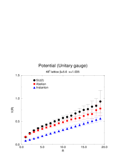
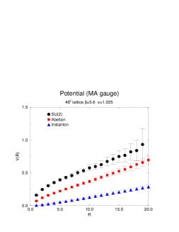
Figure 3: $q$-$\bar{q}$ potential

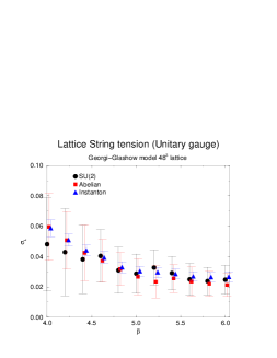
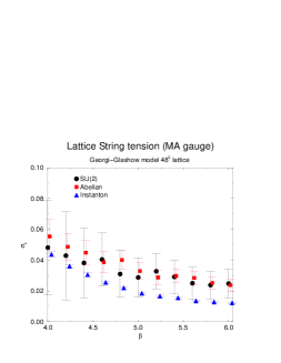
Figure 4: Lattice String tension of Georgi-Glashow model

4.2 Instanton vacuum in both gauges

Polyakov[13] assumed the dilute instanton gas approximation. Let us see the instanton vacuum configurations. As we mention in the previous section, we calculate the instanton configuration using the DeGrand-Toussaint definition. The instanton configuration and anti-instanton configuration in unitary gauge condition for $\beta=4.0$ and $\kappa=1.30$ are shown in Fig.5. Those in MA gauge condition are shown in Fig.6. These configurations look to be a dilute gas for this set of coupling constants.

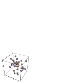
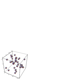
Figure 5: Instanton (left) and anti-instanton (right) vacuum configuration (unitary gauge)

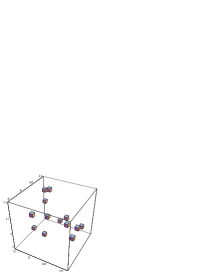
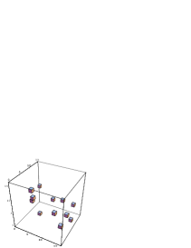
Figure 6: Instanton (left) and anti-instanton (right) vacuum configuration (MA gauge)

Polyakov assumed that instanton charges $q_{a}=\pm 1$ alone contribute to the summation. We plot a histogram of numerically obtained instanton charges in Fig.7 for various blocked instantons. Theoretically an $n$ blocked instanton can take a charge up to $3n^{2}-1$. However as seen from Fig.7, the number of instantons having a charge larger than one is very small. This is consistent with Polyakov’s assumption.

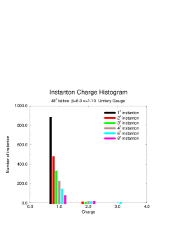
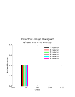
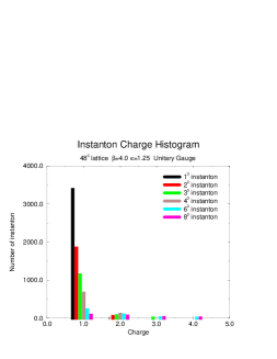
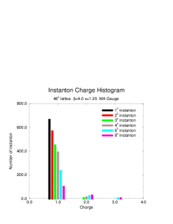
Figure 7: Instanton charge histogram

4.3 Parameter regions of $\beta$ and $\kappa$

Let us discuss here what values of the parameters $\beta$ and $\kappa$ should be chosen. We plot the static potential in Fig.8 for different values of $\kappa$ with fixed $\beta=5.0$ and the instanton density in Fig.9 for $\beta=6.0$.

We see that, in the case of the unitary gauge condition, the instanton density of the system is very large for small $\kappa$, whereas in the case of MA gauge condition it remains low. The dilute gas approximation may be wrong for small $\kappa$ regions in unitary gauge. Actually, the abelian and the instanton potentials have large errors in the unitary gauge, whereas in MA gauge these potentials are seen clearly. The Georgi-Glashow model is reduced to pure $SU(2)$ gauge theory in the limit of $\kappa\rightarrow 0$. Such density and potential behaviors of both gauges are seen also in four-dimensional pure $SU(2)$ gauge theory[16].

What happens in the large $\kappa$ region? One can find that there seems to be a critical $\kappa_{c}$ above which the instanton density becomes vanishing and the instanton contribution to the potential becomes zero. Note that the Georgi-Glashow model in three dimensions is always in the confinement phase contrary to the model in four dimensions. The existence of $\kappa_{c}$ does not mean that instantons are not responsible for confinement. In the limit of $\kappa\rightarrow\infty$, the three-dimensional Georgi-Glashow model becomes the three-dimensional compact U(1) model. The confinement in the latter model is proved to be due to instantons for all $\beta$ region[17]. We can define instantons in the compact U(1) model naturally without following DeGrand and Toussaint (DT). It is those instantons which are responsible for confinement in the compact U(1) model. (We call it as natural instanton.) This concludes that the DT definition of instanton is not good for larger $\kappa$ region than $\kappa_{c}$ in three-dimensional Georgi-Glashow model. In Ref.[8], the effective actions of DT and natural monopoles are studied in 4D compact QED. They are not always in agreement. Hence it is not understandable that the difference appears for such large $\kappa$ and $\beta$ region also in 3D (GG)₃. We admit that the physical meaning of $\kappa_{c}$ is not understood theoretically, however. In this numerical study, we have to adopt the DeGrand-Toussaint definition of instanton, since we do not know how to define natural monopoles in 3D (GG)₃.

Instantons in the unitary gauge are more interesting, since they correspond to the instantons studied by Polyakov[13]. Hence in the following discussions we restrict ourselves to the value of $\kappa$ around $1.0$ which is near but less than $\kappa_{c}$.

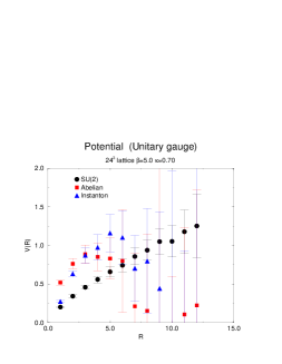
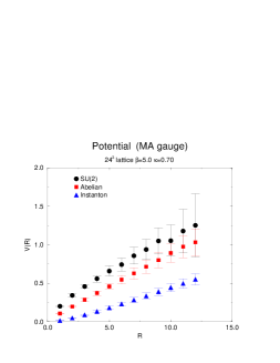
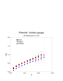
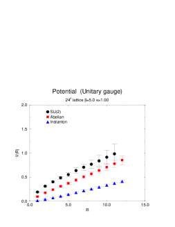
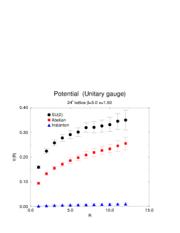
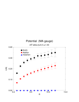
Figure 8: $\kappa$ dependence of $q$-$\bar{q}$ potential

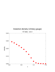
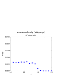
Figure 9: Instanton density

What about the $\beta$ dependence? We show in Fig.10 the $\beta$ dependence for fixed $\kappa=1.00$. For small $\beta$, the static potential for large distance is not fixed clearly. This comes from that the theory in the small $\beta$ region has a large lattice string tension which corresponds to a large lattice distance as shown later. To study the continuum limit, it is better to study larger $\beta$ region.

However, for very large $\beta$, even $\kappa=1.00$ becomes larger than $\kappa_{c}$ in MA gauge. Namely $\kappa_{c}$ depends on the value of $\beta$. When $\beta$ becomes larger, $\kappa_{c}$ becomes smaller. $\kappa_{c}$ in MA gauge is a little bit smaller than that in the unitary gauge. Since we discuss around $\kappa=1.00$, we are restricted to $\beta=4\sim 7$ regions.

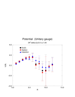
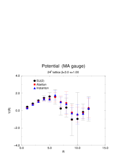
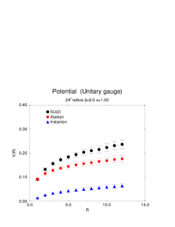
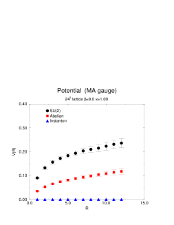
Figure 10: $\beta$ dependence of $q$-$\bar{q}$ potential

4.4 Lattice instanton action

Since the instanton dominance is seen numerically, an effective instanton action is expected to work in the infrared region. Let us derive the lattice instanton action from instanton configurations using Swendsen’s method [15] (See also Appendix B). We express $D(x)$ in (47) as

$$D(x-x^{\prime})=G_{0}\delta^{3}(x-x^{\prime})+G_{1}(\delta^{3}(x-(x^{\prime}-\hat{1}))+...)+G_{2}...,$$ (54)

where we restrict ourselves to ten different two-point couplings shown in Fig.2. Our numerical results are the following:

1. The inverse Monte-Carlo method works very well and the 10 coupling constants are fixed very beautifully. The convergence is very fast.

   When we start from the ensemble of blocked instanton configurations $\{k^{n}(x)\}$, we can get also a lattice action $S[k^{n}]$ very rapidly.

   We have tried to include a four-point self interaction in addition. In the case of $n=1$, we can fix the coupling constants, although the convergence is very slow. The convergence was not obtained in the case $n>1$. Hence we take into account only the two-point interactions.

2. We show in Fig.11 an example of coupling constants in both gauges, where the horizontal axis stands for the distance between two instantons in each two-point interaction. The data points of $S_{8}$ and $S_{9}$ in Fig.11 are almost degenerate.

   The action (28) derived by Polyakov[13] is composed of the self-interaction and the Coulomb term. Hence let us check if the above action obtained numerically can be written similarly as in (28). When we rewrite the lattice Coulomb propagator as

   $$\Delta_{L}^{-1}(x-x^{\prime})=C_{0}\delta^{3}(x-x^{\prime})+C_{1}(\delta^{3}(x-(x^{\prime}-\hat{1}))+...)+C_{2}...,$$ (55)

   we get a beautiful fit

   $${G_{i}}\sim{\rm Const.}\times{C_{i}}~{}(i\neq 0)$$ (56)

   in both gauges as shown in Fig.11.

   The lattice instanton action of Georgi-Glashow model in three-dimension can be written as

   $$S={\rm Self~{}term}+{\rm Const.}\times\sum_{x,x^{\prime}}k(x)\Delta_{L}^{-1}(x-x^{\prime})k(x^{\prime}).$$ (57)

   Although the Coulomb term is reproduced well, we can not compare the self terms of the lattice and the Polyakov actions, since we need to know the details of short-ranged renormalization effects. Actually the lattice Coulomb propagator is finite even at zero distance, whereas the propagator in the continuum is infinite.

   

   

   Figure 11: Coupling constant of lattice instanton action and Coulomb propagator

3. To study the continuum limit, we need to take both $V\to\infty$ and $a\to 0$ limits. First we study the volume dependence of the action, adopting $12^{3},16^{3},24^{3},32^{3}$ and $48^{3}$ lattices. Fig.12 is an example of the lattice volume dependence of couplings for $\beta=4.0,\kappa=1.225$ and $n=2$. In both gauge conditions, the lattice instanton action is almost independent of the lattice volume.

   

   

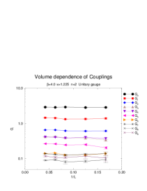
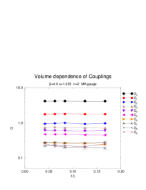
   Figure 12: Volume dependence of Coupling constants

4. We next study the $a\to 0$ limit, performing the block-spin transformation (48). To get the renormalization flow, we have to fix a scale unit. Since there is no physical experimental data in three-dimensional Georgi-Glashow model, we fix the scale in terms of the string tension determined from lattice simulations. The lattice spacing is defined with

   $$a=\sqrt{\frac{\sigma_{L}}{\sigma_{\rm phys}}},$$ (58)

   We perform the block-spin transformations using the scale. An example of the renormalization flow is plotted on the $G_{1}(b)-G_{2}(b)$ and the $G_{2}(b)-G_{3}(b)$ projected planes in Fig.13. We see that there seems to exist a universal flow line especially in the infrared large $b=na(\beta,\kappa)$ region. Each flow line for large $b$ is straight with small errors. The universal flow lines of both gauges are almost the same for large $b$. This suggests the gauge independence of the action in the infrared regions of the continuum limit.

   

   

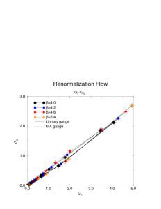
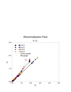
   Figure 13: Flow of Coupling constants

5. To check if the universal curve is the renormalized trajectory which is the continuum theory, let us study a scaling behavior. The continuum limit of the lattice theory is realized when $n\rightarrow\infty$ and $a\rightarrow 0$ for fixed $b$ is taken. Effective actions are usually a function of the step $n$ of the block-spin transformation and the lattice distance $a(\beta,\kappa)$. If the effective action shows a scaling, that is, a function of the product $b=na(\beta,\kappa)$ alone, it is the renormalized trajectory (RT). Since we have seen the couplings except the self one are well reproduced by the Coulomb interaction, let us concentrate on the constant coefficient of the Coulomb term in (57).

   The theory has two parameters $\beta$ and $\kappa$ on the lattice and $g$ and $v$ in the continuum. For the purpose of the comparison with the continuum theory, we tune $\beta$ and $\kappa$ so that we may get the same value of $v=\sqrt{\kappa/a(\beta,\kappa)}$ as in Table.2. Here we fix $v\sim 2.56$. The values of the parameters $\beta$ and $\kappa$ in Table 1 are chosen similarly.

   $\beta$	$\kappa$	$v$	$\kappa$	$v$	$\kappa$	$v$
   6.0	1.030	2.549(68)
   5.8	1.030	2.552(61)	1.005	2.419(62)	1.015	2.519(65)
   5.6	1.035	2.554(66)
   5.4	1.055	2.566(62)	1.050	2.443(67)	1.065	2.656(65)
   5.2	1.065	2.567(63)	1.065	2.468(68)	1.080	2.588(58)
   5.0	1.065	2.549(66)	1.095	2.621(63)	1.100	2.704(60)
   4.8	1.090	2.544(61)	1.105	2.481(65)	1.120	2.623(49)
   4.6	1.140	2.549(65)	1.150	2.602(64)
   4.4	1.170	2.553(51)	1.160	2.441(59)	1.175	2.612(61)
   4.2	1.210	2.548(50)	1.195	2.515(62)
   4.0	1.255	2.549(60)	1.225	2.488(56)

   Table 2: Parameters of $\beta$ and $\kappa$ for fixed $v$.

   Then we study in Fig.14 $n$ dependence for some $b$.

   

   

   Figure 14: $n$ dependence of Coulomb term

   One can find that the action for $n\geq 4$ blocked instantons looks on RT. The scaling can be seen more clearly in Fig.15 in which we show the Coulomb term vs. $b$ for fixed $v\sim 2.56$. This is very interesting.

   

   Figure 15: Proportional coefficient of Coulomb term

6. Let us determine the gauge coupling $g$ which is super-renormalizable in three dimensions. For that purpose, let us rewrite the action, restoring the lattice spacing $b=na$ explicitly:

   $$S[k] = \sum_{x,x^{\prime}}b^{6}k(bx)D(bx-bx^{\prime})k(bx^{\prime})$$ (59)

   $$= {\rm Self~{}term}+\beta_{m}\sum_{x,x^{\prime}}b^{6}k(bx)\Delta_{L}^{-1}(bx-bx^{\prime})k(bx^{\prime}),$$

   where $\beta_{m}$ is a constant. Since the mass dimension of the lattice Coulomb propagator is $1$ and that of $\delta^{3}(bx-bx^{\prime})$ is $3$, the coefficients $C_{i}$ in (55) have the mass dimension $2$. $\beta_{m}$ is written as $8\pi/g^{2}$. Hence the constant in (57) is expected to behave as

   $${\rm Const.}\sim\frac{8\pi}{g^{2}}\frac{1}{b^{2}}.$$ (60)

   The $1/b^{2}$ behavior in each gauge is actually observed for $b>1$ as shown in Fig.15. ¿From the fitting (60), we can obtain the renormalized gauge coupling $g$ numerically. In the case of $v\sim 2.56$, we find $g=3.9(2)$ in the unitary gauge condition and $g=3.8(1)$ in MA gauge. Gauge independence is seen also in this case.

4.5 String tension of the Polyakov model

Now let us calculate the string tension $\sigma_{\rm cl}=Mg^{2}/(4\pi)$ of Polyakov’s model (27) using the lattice parameters determined from the renormalized trajectory.

Note that

$$M^{2}=2\left(\frac{4\pi}{g}\right)^{2}N^{3/2}m_{W}^{3}e^{-\frac{m_{W}}{g^{2}}\epsilon(\lambda/g^{2})}$$ (61)

and

$$N=\frac{m_{W}}{g^{2}}\alpha(\lambda/g^{2}).$$ (62)

As evaluated in Sec.2, we get $\epsilon(\infty)=4\pi\times 1.67$ and $\alpha(\infty)\simeq 4\pi\times 3.33$. Also we have seen above that, for $v\sim 2.56$, $g=3.9(2)$ in the unitary gauge and $g=3.8(1)$ in MA gauge.

Using these parameters, we can estimate the string tension from Eq.(27). In the case of the unitary gauge condition,

$$\sqrt{\frac{\sigma_{\rm cl}}{\sigma_{L}}}=1.4(9)({\rm unitary~{}gauge}).$$ (63)

Note that we are considering the scale using $\sigma_{L}$. The error is not small, since the errors of $g$ and $v$ is enlarged by the exponential factor in Eq.(16).

In the case of MA gauge, we obtain

$$\sqrt{\frac{\sigma_{\rm cl}}{\sigma_{L}}}=1.3(8)({\rm MA~{}gauge}).$$ (64)

Considering the fact that the saddle point approximation used in deriving Eq.(27) is not perfectly justified for such small $g$ used here, the above agreement is rather surprising. In conclusion, we may say that the confinement scenario of three-dimensional Georgi-Glashow model by Polyakov is thus verified numerically.

5 Concluding remarks

We have studied three-dimensional lattice Georgi-Glashow model in the London limit $\lambda\to\infty$ under the restriction to an intermediate region where the screening appears. In Ref.[14], the screening is seen around the range of $O(2m_{W}/\sigma)$. In our case this value is around 20 in our unit. As seen in Fig.15, we are dealing with the region up to $b\sim 2$ in our unit. Hence the screening is not viable in this region.

We have found that Polyakov’s quasi-classical analyses on the basis of the dilute instanton gas approximation are in almost quantitative agreement with the Monte-Carlo results using the DeGrand-Toussaint definition of a lattice instanton both in the unitary and the MA gauges.

There are other exciting topics to which one can apply the method developed here.

1. When we integrate out non-zero modes of gauge and quark fields perturbatively in high temperature QCD in four dimensions, we get an effective model described in terms of the zero-mode bosonic fields alone. The model is equivalent to the three-dimensional Georgi-Glashow model [18]. The effective couplings $g$, $v$ and $\lambda$ are calculated in terms of the quantities in four-dimensional QCD. In this case we need to perform simulations for the case with finite $\lambda$. It is very interesting to know if non-perturbative effects in the deconfinement phase of (QCD)₄ can be explained totally by the instanton effects.

2. It is expected that, when $\lambda=0$, the three-dimensional Georgi-Glashow model can not be described in terms of the Coulomb gas of instantons and the deconfinement phase will appear[19]. There is an attractive interaction between instantons and anti-instantons which does not depend on the sign of the magnetic charge. It is a Yukawa-type interaction for $\lambda\neq 0$. But when $\lambda=0$, the Higgs field becomes massless and the interaction just cancel the Coulomb repulsive interaction between the same-sign instantons or between anti-instantons. However, such a scenario needs information of the core region of instantons and so non-perturbative numerical evaluation is highly desirable.

Appendix A Confinement from the instanton dilute gas model

String tension from the dilute gas model Eq.(27) is calculated as follows.

Let us start from Eq.(24):

$$Z[\eta]=\int D\chi\exp{\left\{-\frac{1}{2}\left(\frac{g}{4\pi}\right)^{2}\int{\rm d}^{3}x[(\partial_{\mu}(\chi-\eta))^{2}-2M^{2}\cos{\chi}]\right\}},$$ (65)

$$\eta(x)=\int_{S}{\rm d}\vec{S}\cdot\frac{\vec{x}-\vec{y}}{|\vec{x}-\vec{y}|^{3}}.$$ (66)

The path integral may be evaluated by the saddle point approximation when the coupling $g$ is large enough. Then we have to solve the saddle point equation

$$\partial^{2}(\chi_{\rm cl}-\eta)=M^{2}\sin{\chi_{\rm cl}}.$$ (67)

We assume a Wilson loop that the contour $C$ is planar and is placed in the $xy$ plane as in Fig.16 .

Figure 16: Wilson loop

Then Eq.(67) takes the form

$$\partial^{2}\chi_{\rm cl}=2\pi\delta(z)\theta_{S}(xy)+M^{2}\sin{\chi_{\rm cl}},$$ (68)

where

$$\theta_{S}(xy)=\left\{\begin{array}[]{cl}1&~{}~{}~{}~{}x,y\in S\\ 0&~{}~{}~{}~{}{\rm otherwise}\end{array}\right..$$ (69)

Far from the boundaries of the contour, Eq.(68) is approximately one dimensional ($\chi_{\rm cl}$ depends only on $z$) and has a solution

$$\chi_{\rm cl}=\left\{\begin{array}[]{cc}~{}4\arctan(e^{-Mz})&z>0\\ -4\arctan(e^{Mz})&z<0\end{array}\right..$$ (70)

$\eta(x)$ only depends on $z$ approximately, too. Eq.(25) is rewritten as

$$\eta(x) = \int_{-r}^{r}{\rm d}y_{1}\int_{-t}^{t}{\rm d}y_{2}\frac{x_{3}}{\{(x_{1}-y_{1})^{2}+(x_{2}-y_{2})^{2}+{x_{3}}^{2}\}^{3/2}}$$

$$= \arctan\left(\frac{(r-x_{1})(t-x_{2})}{x_{3}\sqrt{(x_{1}-r)^{2}+(x_{2}-t)^{2}+{x_{3}}^{2}}}\right)$$

$$+\arctan\left(\frac{(r+x_{1})(t-x_{2})}{x_{3}\sqrt{(x_{1}+r)^{2}+(x_{2}-t)^{2}+{x_{3}}^{2}}}\right)$$

$$+\arctan\left(\frac{(r-x_{1})(t+x_{2})}{x_{3}\sqrt{(x_{1}-r)^{2}+(x_{2}+t)^{2}+{x_{3}}^{2}}}\right)$$

$$+\arctan\left(\frac{(r+x_{1})(t+x_{2})}{x_{3}\sqrt{(x_{1}+r)^{2}+(x_{2}+t)^{2}+{x_{3}}^{2}}}\right).$$

Now, if $r\gg x_{1}$ and $t\gg x_{2}$ ( far from the boundaries of the contour), it is reduced to

$$\eta(z)\sim 4\arctan\left(\frac{rt}{z\sqrt{r^{2}+t^{2}+z^{2}}}\right).$$ (71)

Hence, one may estimate the integral of $Z[\eta]$ in terms of a $z$ integral alone(where $x_{3}\rightarrow z$ ):

$$Z[\eta]\sim\exp\left\{\frac{1}{2}\left(\frac{g}{4\pi}\right)^{2}SM^{2}\int{\rm d}z[(\chi_{\rm cl}(z)-\eta(z))\sin\chi_{\rm cl}+\cos\chi_{\rm cl}]\right\},$$ (72)

where $S$ is the area of the Wilson loop ($S=R\cdot T=4rt$).

¿From Eq.(25), (72) and (71),

$$W[C] \sim \exp\left\{-RT\left(\frac{g}{4\pi}\right)^{2}M^{2}\right.$$ (73)

$$\left.\int_{0}^{\infty}{\rm d}z\left[16\arctan\left(\frac{rt}{z\sqrt{r^{2}+t^{2}+z^{2}}}\right)\frac{e^{-Mz}(1-e^{-2Mz})}{(1+e^{-2Mz})^{2}}\right]\right\}.$$

The string tension is given by

$$\sigma_{\rm cl}=M\left(\frac{g}{\pi}\right)^{2}\int_{0}^{\infty}{\rm d}z\left[\arctan\left(\frac{M^{2}rt}{z\sqrt{(Mr)^{2}+(Mt)^{2}+z^{2}}}\right)\frac{e^{-z}(1-e^{-2z})}{(1+e^{-2z})^{2}}\right].$$ (74)

The $z$ integral of Eq.(74) is finite if $Mr,Mz\rightarrow\infty$ . Thus we obtain the string tension Eq.(27)

$$\sigma_{\rm cl}=\frac{Mg^{2}}{4\pi}.$$ (75)

Appendix B Swendsen’s method

We determine a lattice instanton action from instanton configurations on three-dimensional lattice. A theory of instanton is given in general by the following partition function

$$Z=\left(\prod_{x}\sum_{k(x)=-\infty}^{+\infty}\right)~{}e^{-S[k]},$$ (76)

where $S[k]$ is an instanton action describing the theory. Consider a set of all independent operators which are summed up over the whole lattice. We denote each operator as $S_{i}[k]$. Then, the action may be written as a linear combination of these operators,

$$S[k]=\sum_{i}G_{i}S_{i}[k],$$ (77)

where $G_{i}$ are renormalized coupling constants.

The expectation value of operator ${\cal O}[k]$ is estimated as

$$<{\cal O}[k]>=\frac{1}{Z}\left(\prod_{x}\sum_{k(x)=-\infty}^{+\infty}\right){\cal O}[k]~{}e^{-S[k]}.$$ (78)

Here, we focus on a certain site $x^{\prime}$. We define $\hat{S}[k]$ which contains $k(x^{\prime})$ and rewrite the numerator of Eq.(78) as

$$\left(\prod_{x}\sum_{k(x)=-\infty}^{+\infty}\right){\cal O}[k]e^{-S[k]}$$ (79)

$$=\left({\prod_{x}}^{\prime}\sum_{k(x)=-\infty}^{+\infty}\right)~{}e^{-\sum_{i}G_{i}(S_{i}[k]-\hat{S}_{i}[k])}\{\sum_{k(x^{\prime})=-\infty}^{+\infty}{\cal O}[k]~{}e^{-\sum_{i}G_{i}\hat{S}_{i}[k]}\},$$ (80)

where ${\prod}^{\prime}$ means the product except for the site $x^{\prime}$. We rewrite Eq.(80) as

$$(\ref{exp-Z21}) = \left({\prod_{x}}^{\prime}\sum_{k(x)=-\infty}^{+\infty}\right)~{}e^{-\sum_{i}G_{i}(S_{i}[k]-\hat{S}_{i}[k])}$$ (81)

$$~{}~{}~{}\sum_{k(x^{\prime})=-\infty}^{+\infty}\frac{\sum_{\hat{k}=-\infty}^{+\infty}{\cal O}[\hat{k},\{k\}^{\prime}]~{}e^{-\sum_{i}G_{i}\hat{S}_{i}[\hat{k},\{k\}^{\prime}]}}{\sum_{\hat{k}=-\infty}^{+\infty}e^{-\sum_{i}G_{i}\hat{S}_{i}[\hat{k},\{k\}^{\prime}]}}~{}~{}e^{-\sum_{i}G_{i}\hat{S}_{i}[k]}$$

$$= \left(\prod_{x}\sum_{k(x)=-\infty}^{+\infty}\right)\hat{\cal O}[k]~{}e^{-\sum_{i}G_{i}S_{i}[k]},$$

where

$$\hat{\cal O}[k]=\frac{\sum_{\hat{k}=-\infty}^{+\infty}{\cal O}[\hat{k},\{k\}^{\prime}]~{}e^{-\sum_{i}G_{i}\hat{S}_{i}[\hat{k},\{k\}^{\prime}]}}{\sum_{\hat{k}=-\infty}^{+\infty}e^{-\sum_{i}G_{i}\hat{S}_{i}[\hat{k},\{k\}^{\prime}]}},$$ (82)

$\hat{k}=k(x^{\prime})$ and $\{k\}^{\prime}$ is the coset of $\hat{k}$.

When we consider the DeGrand-Toussaint definition of instanton, the sum with respect to instanton charge in Eq.(82) is not $[-\infty,+\infty]$ but to $[-(3n^{2}-1),3n^{2}-1]$, where $n$ is a step of block spin transformation of instanton.

Hence we get an identity

$$<{\cal O}[k]>=<\hat{\cal O}[k]>.$$ (83)

Since we don’t know the correct set of coupling constants $G_{i}$, we have to start from a trial set of coupling constants $\tilde{G}_{i}$ . We define $\overline{\cal O}[k]$ in which the true coupling constants $G_{i}$ in Eq.(82) are replaced by the trial ones $\tilde{G}_{i}$ as

$$\overline{\cal O}[k]=\frac{\sum_{\hat{k}=k_{\rm min}}^{k_{\rm max}}{\cal O}[\hat{k},\{k\}^{\prime}]~{}e^{-\sum_{i}\tilde{G}_{i}\hat{S}_{i}[\hat{k},\{k\}^{\prime}]}}{\sum_{\hat{k}=k_{\rm min}}^{k_{\rm max}}~{}e^{-\sum_{i}\tilde{G}_{i}\hat{S}_{i}[\hat{k},\{k\}^{\prime}]}}.$$ (84)

If the trial $\tilde{G}_{i}$ are not equal to the true $G_{i}$, $<{\cal O}[k]-\overline{\cal O}[k]>\neq 0$. When $\{\tilde{G}_{i}\}$ are not far from $\{G_{i}\}$, we get

$$<{\cal O}[k]-\overline{\cal O}[k]>\sim\sum_{i}<\overline{\cal O}~{}\overline{S}_{i}-(\overline{{\cal O}S_{i}})>(G_{i}-\tilde{G}_{i}).$$ (85)

Actually, if we use $S_{i}[k]$ as an operator ${\cal O}[k]$, we get a very good convergence . Hence we use here

$$<S_{i}[k]-\overline{S}_{i}[k]>\sim\sum_{j}<\overline{S}_{i}~{}\overline{S}_{j}-(\overline{S_{i}S_{j}})>(G_{j}-\tilde{G}_{j}).$$ (86)

Since the value of $S_{i}[k]$ is obtained from vacuum configurations, we can solve Eq.(86) iteratively to obtain the real set of coupling constants $G_{i}$.

References

- [1] K. G. Wilson, Phys. Rev. D10 (1974) 2445.
- [2] S. Mandelstam, Phys. Rep. 23C (1976) 245.
- [3] G. ’t Hooft, High Energy Physics ed. A. Zichichi (Editorice Compositori, Bologna, 1975).
- [4] G. ’t Hooft, Nucl. Phys. B190 (1981) 455.
- [5] T. Suzuki and I. Yotsuyanagi, Phys. Rev. D42 (1990) 4257.
- [6] T. A. DeGrand and D. Toussaint, Phys. Rev. D22 (1980) 2478.
- [7] H. Shiba and T. Suzuki, Phys. Lett. B333 (1994) 461.
- [8] H. Shiba and T. Suzuki, Phys. Lett. B343 (1995) 315 , and Phys. Lett. B351 (1995) 519.
- [9] S. Kato, S. Kitahara, N. Nakamura and T. Suzuki, Nucl. Phys. B520 (1998) 323.
- [10] S. Fujimoto, S. Kato and T. Suzuki, Phys. Lett. B476 (2000) 437.
- [11] G. ’t Hooft, Nucl. Phys. B79 (1974) 276.
- [12] A. M. Polyakov, Phys. Lett. 59B (1975) 82.
- [13] A. M. Polyakov, Nucl. Phys. B120 (1977) 429.
- [14] J.Ambjørn and J.Greensite, JHEP 05 (1998) 004.
- [15] R. H. Swendsen, Phys. Rev. Lett. 52 (1984) 1165; Phys. Rev. B30(1984) 3866,3875.
- [16] T. Suzuki, Nucl. Phys. B (Proc. Suppl.) 30. 176 (1993).
- [17] T. Banks, R. Myerson and J. Kogut, Nucl. Phys. B129 (1977) 493.
- [18] P. Lacock, D. E. Miller and T. Reisz, Nucl. Phys. B369 (1992) 501.
- [19] S. F. Magruder, Phys. Rev. D17 (1978) 3257.