Abstract

I review the status of lattice simulations relevant for phenomenological studies of $B$-physics. Results for much-studied quantities such as $f_{B}$, $B_{B}$ and form-factors for semileptonic decays are presented as well as those for quantities which have begun to be studied only recently (such as $B$-lifetimes). The improvement in the precision of the determinations of the mass of the $b$-quark, which has been made possible by new results for perturbative coefficients, is discussed. Finally I describe new ideas being developed with the aim of making computations of two-body non-leptonic decays possible.

1 Introduction

At this conference we have seen a huge amount of experimental data being presented on $B$-physics, data from which we would like to extract fundamental information about the parameters of the standard model and CP-violation, and (by overconstraining the comparison with the standard model) to search for signals of new physics. Of course much more data will become available in the coming years. A major difficulty in achieving the above goals is our inability to quantify non-perturbative strong interaction effects. Lattice QCD provides the opportunity for evaluating these effects ab initio, and there is indeed a wide-ranging program of numerical simulations of $B$-physics. In this lecture I will briefly review some of the recent progress in lattice studies of $B$-physics.

It is not appropriate for me in this talk to discuss technical aspects of lattice calculations in any detail, I will therefore concentrate on presenting results and discussing the potential for future calculations. I start with some basic facts about lattice calculations in $B$-physics. In any simulation the computing resources are limited, and one therefore has to compromise when minimising competing systematic errors, those due to the granularity of the lattice (discretization effects) and finite-volume errors. In current simulations, this typically leads to a choice for the lattice spacing ($a$) in the range given by $a^{-1}\sim 2$ – 4 GeV, i.e. $a$ is larger than the Compton wavelength of the $b$-quark. This means that we cannot study the propagation of a physical $b$-quark directly and either have to i) use effective theories, such as the Heavy Quark Effective Theory (HQET) or Non-Relativistic QCD (NRQCD) or ii) calculate physical quantities with the heavy-quark mass $m_{Q}$ in the region of $m_{c}$ (the mass of the charm-quark), and perform the extrapolation to $m_{Q}=m_{b}$.

The precision of lattice calculations is limited by systematic uncertainties. These can be overcome in principle with increased computing resources and much effort is being devoted to reducing these uncertainties (and in particular to eliminating quenching, i.e. to include vacuum polarisation effects). Most, but not all, of the results presented below have been obtained in the quenched approximation. It should be remembered however, that even in unquenched simulations the masses of the sea quarks are large . Controlling the effects of sea-quarks is perhaps the major challenge for the lattice community and in recent years we have began to address this challenge.

From lattice simulations we know how to calculate matrix elements of the form $\langle H\,|\,O(0)\,|\,0\rangle$ and $\langle\,H_{1}\,|\,O(0)\,|\,H_{2}\,\rangle$, where $H$ and $H_{1,2}$ are hadrons and $O(0)$ is some local composite operator (several examples of such matrix elements will be discussed below). We are not yet in a position to compute matrix elements in which there are two or more hadrons in the initial or final state, and are therefore unable to compute $B\to H_{1}H_{2}$ decays amplitudes, but progress is being made in this area (see sect. 5 below).

The plan of this lecture is as follows. In the next section I briefly review the results for some standard physical quantities: leptonic decay constants $f_{B}$ and $f_{B_{s}}$; the $B_{B}$-parameters of $\bar{B}$-$B$ mixing and form-factors for semileptonic decays. Sect. 3 contains a discussion of computations of inclusive decays and lifetimes. Results have been recently obtained for these quantities but they have not been studied as extensively as those in sect. 2. New calculations of perturbative coefficients have enabled the mass of the $b$-quark to be determined from lattice simulations with considerably better precision and this is reviewed in sect. 4. I then describe recent attempts to develop techniques to enable two-body non-leptonic decays to be studied on the lattice (sect. 5). Finally I summarise the main conclusions in sect. 6.

2 Decay Constants, B–Parameters and Form-Factors

Leptonic decay constants $f_{B}$ and $f_{B_{s}}$, the $B$–parameters of $B$–$\bar{B}$ mixing and the form-factors for semileptonic $B$-decays have been computed in lattice simulations for over ten years now. In this section I briefly discuss each of these quantities in turn.

2.1 $\mathbf{f_{B}}$

The strong interaction effects in leptonic decays of $B$–mesons (see fig.1) are contained in the matrix element

$$\langle\,0\,|\,A_{\mu}(0)\,|\,B(p)\,\rangle=if_{B}p_{\mu}\ .$$ (1)

Lorentz and Parity Invariance imply that all the non-perturbative QCD effects are parametrized in terms of a single number, $f_{B}$, defined in eq.(1).

Figure 1: Diagrammatic representation of a leptonic decay of a $B$–meson.

Claude Bernard, the reviewer at the Lattice 2000 symposium [1] summarised the current status of the results as :

	Full Theory	$N_{f}=0$
$f_{B}$	$200\pm 30$ MeV	$175\pm 20$ MeV
$f_{B_{s}}/f_{B}$	$1.16\pm 0.04$	$1.15\pm 0.04$

At last year’s conference the reviewer S.Hashimoto stated that all available data is consistent with the following estimates: [2]

	$N_{f}=2$	$N_{f}=0$
$f_{B}$	$210\pm 30$ MeV	$170\pm 20$ MeV
$f_{B_{s}}$	$245\pm 30$ MeV	$195\pm 20$ MeV
$f_{B_{s}}/f_{B}$	$1.16\pm 0.04$	$1.15\pm 0.04$

These results have been largely stable for some time. The last time that I performed a compilation was in 1997 together with Jonathan Flynn [3] and reported (on what were mainly quenched calculations):

$$f_{B}=170\pm 35\,\textrm{MeV},\ \ f_{B_{s}}=195\pm 35\,\textrm{MeV},\ \ \frac{f_{B_{s}}}{f_{B}}=1.14\pm 0.08.$$ (2)

Although the results have been stable, the errors have been decreasing very slowly (if at all). The errors will not decrease significantly until we begin to get a serious control of quenching errors. In unquenched calculations, the value of the lattice spacing typically varies by 10% or so depending on the physical quantity which is used to set the scale. It is therefore not really possible to determine dimensionful quantities such as $f_{B}$ with a better precision than about 10%.

In the last two years we have began to study quenching effects, although it must be remembered that at present the masses of the sea-quarks are still relatively heavy (typically a little smaller that the strange quark mass). These effects can only be studied meaningfully if all other variables are kept constant. Using results from the MILC [4], CPPACS [5] and NRQCD [6] collaborations, C. Bernard estimates that there is about a 20 MeV increase in the value of $f_{B}$ in going from the quenched approximation to the $N_{f}=2$ case (using $f_{\pi}$ to set the scale) [1]. The value of $f_{B_{s}}/f_{B}$ appears to be the same in the two cases.

Although the errors have not been reduced substantially, there have been many systematic checks on the stability of the results. For example discretization errors have been studied by using improved actions and/or extrapolating the results to the continuum limit. It had been suggested that $f_{B}$ may be significantly lower than the results presented above because of discretization errors (this suggestion was based on some extrapolations to the chiral limit), but this has not survived more careful analyses [1].

When lattice computations of the leptonic decay constants of heavy mesons were beginning there were no experimental data. In 1997 we compiled the (quenched) lattice predictions for the decays constants of charmed mesons as [3]:

$$f_{D}=200\pm 30\,\textrm{MeV\ \ and\ \ }f_{D_{s}}=220\pm 30\,\textrm{MeV}.$$ (3)

The Particle Data Group’s review this year quotes $f_{D_{s}}=280\pm 19\pm 28\pm 34$ MeV [7] as the best experimental result (and recent results, still with large errors, are compatible with this). It will be interesting to observe future lattice and experimental results as the errors in both decrease.

Finally let me mention that lattice computations have shown that there are large corrections to the HQET scaling law for the decay constants of heavy-light pseudoscalar mesons $P$

$$f_{P}\sim\frac{1}{\sqrt{m_{P}}}.$$ (4)

2.2 $\mathbf{B_{B}}$:

The relevant matrix element for $B^{0}$-$\bar{B}^{0}$ mixing is:

$$M(\mu)\equiv\langle\,\bar{B}^{0}\,|\,\bar{b}\gamma_{\mu}(1-\gamma_{5})q\ \bar{b}\gamma^{\mu}(1-\gamma_{5})q\,|\,B^{0}\,\rangle\,,$$

where $q$ represents $d$ or $s$. This is illustrated in fig. 2.

Figure 2: Diagramatic representation of $B^{0}$-$\bar{B}^{0}$ mixing.

Following the conventions introduced in kaon physics, B-parameters are defined by

$$M(\mu)=\frac{8}{3}f_{B}^{2}m_{B}^{2}B_{B}(\mu).$$ (5)

$B_{B}(\mu)$ is scheme and scale-dependent, so it is convenient to define a renormalization scheme and scale- independent (up to NLO) quantity

$$\hat{B}_{B}^{\textrm{nlo}}=\alpha_{s}(\mu)^{2/\beta_{0}}\left[1\,+\,\frac{\alpha_{s}(\mu)}{4\pi}\,J_{n_{f}}\right]\ B_{B}(\mu).$$ (6)

where $J_{n_{f}}$ is a known constant. Many groups have studied mixing in lattice simulations and C. Bernard, the reviewer at this year’s lattice conference, summarised the results as:

$$\hat{B}_{B_{d}} = 1.30\pm 0.12\pm 0.13,\hskip 36.135pt\hat{B}_{B_{s}}/\hat{B}_{B_{d}}=1.00\pm 0.04\,,$$ (7)

$$f_{B}\sqrt{\hat{B}_{B_{d}}} = 230\pm 40\,\textrm{MeV},\hskip 36.135pt\xi\equiv\frac{f_{B_{s}}\sqrt{\hat{B}_{B_{s}}}}{f_{B}\sqrt{\hat{B}_{B_{d}}}}=1.16\pm 0.05\,.$$ (8)

The second error for $B_{B_{d}}$ is an estimate of the error due to quenching. $\xi$ is a particularly important quantity for studies of the unitarity triangle. It should be noted that the error on $\xi$ is not a small one from the lattice perspective, indeed given its central importance in phenomenological studies most groups tend to be cautious in determining this error. The reason that it should not be considered small is that the quantity which is being computed is $\xi-1=0.16\pm 0.05$, i.e. it has a quoted error of over 30%. In my judgement therefore the uncertainty in the value of $\xi$ should not be further inflated in phenomenological studies. The results for $\xi$ are stable, and there is no evidence that they change as sea-quarks are introduced.

For comparison with the results quoted above I present also those quoted in our 1997 review [3]:

$$\hat{B}_{B_{d}} = 1.4\pm 0.1,\hskip 36.135pt\hat{B}_{B_{d}}/\hat{B}_{B_{s}}=1.01\pm 0.01\,,$$ (9)

$$f_{B}\,\sqrt{\hat{B}_{B_{d}}} = 201(42)\,\textrm{MeV}\,,\hskip 36.135pt\xi\equiv\frac{f_{B_{s}}\sqrt{\hat{B}_{B_{s}}}}{f_{B}\sqrt{\hat{B}_{B}}}=1.14\pm 0.08.$$ (10)

These results have been obtained with propagating heavy quarks (i.e. by extrapolating results obtained with $m_{Q}\simeq m_{c}$). In the static approximation the perturbative corrections are very large and hence these have not given us much useful information to date.

2.3 Exclusive Semi-Leptonic $B$-Decays

Exclusive semileptonic decays of $B$-mesons are being used to determine the $V_{cb}$ and $V_{ub}$ CKM-matrix elements. Diagramatically the amplitudes can be represented by the diagram in fig. 3.

Figure 3: Diagramatic Representation of Semileptonic B-Decays.

Lorentz and parity invariance imply that the amplitudes can be expressed in terms of invariant form factors. For example for the decays into a pseudoscalar $P$ ($B\to\pi$ or $B\to D$ decays), in the helicity basis,

$$\langle\,P(p_{P})\,|V_{\mu}(0)\,|\,B(p_{B})\,\rangle=f^{0}(q^{2})\,\frac{M_{B}^{2}-M_{P}^{2}}{q^{2}}q_{\mu}+f^{+}(q^{2})\,\left\{(p_{B}+p_{P})_{\mu}-\frac{M_{B}^{2}-M_{P}^{2}}{q^{2}}q_{\mu}\right\}.$$ (11)

As a result of parity invariance only the vector component (from the $V-A$ weak current) contributes in this case. When the final-state hadron is a vector meson ($\rho$ or $D^{\ast}$) the amplitude is written in terms of four invariant form factors.

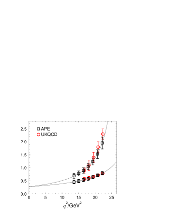
Figure 4: The left-hand diagram shows results for $f^{+}$ (upper points) and $f^{0}$ (lower points) from the APE [8] and UKQCD [9] collaborations. The curves are fits to the points from APE, showing an extrapolation to lower values of $q^{2}$. The right-hand diagram shows the UKQCD results for the distribution for $b\to\rho$ decays in the range $14$ GeV${}^{2}<q^{2}<20.3$ GeV², which corresponds to the high $q^{2}$ bin of CLEO. The region marked phase space only is inaccessible to the lattice calculations and the curve corresponds to taking the form-factors from the last lattice point and extrapolating using the phase-space only.

I will only make a few brief comments about semileptonic decays:

• Lattice simulations of $B\to\pi,\rho$ decays require the momentum of the final-state light meson to be small in order to avoid discretization errors. This means that from lattice simulations of $B\to\pi,\rho$ semileptonic decays we only obtain results at large values of $q^{2}$. This is illustrated by the first diagram in fig. 4, which contains recent data from the APE [8] and UKQCD collaborations [9] .

• Lattice computations of semileptonic form-factors have been performed for many years now. At the lattice 2000 symposium updated results were presented from the APE, UKQCD, JLQCD and Fermilab collaborations and “the results were fairly consistent in the region where all groups had direct calculations (19 GeV${}^{2}<\,q^{2}\,<\,23\,$GeV²)” [1]. As an example, the first diagram in fig. 4 shows the results for the form factors $f^{+}$ and $f^{0}$ for $B\to\pi$ decays.

• Much effort is being devoted to extrapolating the lattice results to smaller values of $q^{2}$, using as many theoretical constraints as possible (e.g. HQET scaling relations, unitarity and analyticity, kinematical constraints, soft pion relations etc.) [10]. The results of such extrapolations for $f^{0}$ and $f^{+}$ are also shown in fig. 4.

• For a direct application of lattice computations one should compare the lattice results to experimental distributions at large values of $q^{2}$. An example of such a comparison is shown in the second diagram in fig.4, where the lattice results from the UKQCD collaboration for $B\to\rho$ decays [9] are compared with the high-$q^{2}$ bin from CLEO [11]. Integrating the results in this bin the comparison takes the form:

  $$\frac{\Delta\Gamma(14<q^{2}/\,\mathrm{Ge\kern-1.00006ptV}^{2}<20.3)}{\mathrm{ps}^{-1}\,\mathrm{Ge\kern-1.00006ptV}^{-2}} = 8.3\,|V_{ub}|^{2}\hskip 46.25275pt\textrm{UKQCD\ preliminary}$$ (12)

  $$= 7.1(2.4)\times 10^{-5}\hskip 14.45377pt\textrm{CLEO}$$ (13)

  from which one obtains $V_{ub}=2.9(0.5)\times 10^{-3}$.

3 Inclusive Decays and Lifetimes of Beauty Hadrons

In this section I will briefly mention some physical quantities for which the first lattice calculations were performed in the last few years. It will certainly be possible to improve on the precision of these first-generation computations.

3.1 Lifetimes of Beauty Hadrons:

The fact that the $b$-quark is heavy makes it possible to derive an operator product expansion for inclusive beauty decays [12], which results in an expansion in inverse powers of $m_{b}$. Specifically for widths of beauty hadrons:

$$\Gamma(H_{b})=\frac{G_{F}^{2}\,m_{b}^{5}\,|V_{cb}|^{2}}{192\pi^{3}}\left\{c_{3}\left(1+\frac{\lambda_{1}+3\lambda_{2}}{2m_{b}^{2}}\right)+c_{5}\frac{\lambda_{2}}{m_{b}^{2}}+O\left(\frac{1}{m_{b}^{3}}\right)\right\}$$ (14)

where $c_{3}$ and $c_{5}$ are calculable in perturbation theory and

$$-\lambda_{1}=\frac{1}{2m_{H_{b}}}\ \langle\,H_{b}\,|\,\bar{h}\vec{D}^{2}h\,|\,H_{b}\,\rangle\ \ \ \textrm{and}\ \ \ 3\lambda_{2}=\frac{1}{2m_{H_{b}}}\ \langle\,H_{b}\,|\,\frac{g}{2}\,\bar{h}\sigma_{ij}G^{ij}h\,|\,H_{b}\,\rangle$$ (15)

defined in the rest frame of $H_{b}$ ($\lambda_{1}$ and $\lambda_{2}$ are the matrix elements of the kinetic energy and chromomagnetic operators respectively). This leads to

$$\frac{\tau(B^{-})}{\tau(B^{0})} = 1\,+\,O\left(\frac{1}{m_{b}^{3}}\right)$$ (16)

$$\frac{\tau(\Lambda_{b})}{\tau(B^{0})} = 1\,-\,\frac{\lambda_{1}(\Lambda_{b})-\lambda_{1}(B^{0})}{2m_{b}^{2}}\,+\,3\,c_{G}\frac{\lambda_{2}(\Lambda_{b})-\lambda_{2}(B^{0})}{m_{b}^{2}}+\cdots$$ (17)

$$= (0.98\pm 0.01)+\,O\left(\frac{1}{m_{b}^{3}}\right),$$ (18)

to be compared to the experimental values 

$$\frac{\tau(B^{-})}{\tau(B^{0})}=1.06\pm 0.04\ \ \textrm{and}\ \ \frac{\tau(\Lambda_{b})}{\tau(B^{0})}=0.79\pm 0.05\ .$$ (19)

In view of the discrepancy between the theoretical prediction in (18) and the experimental results for the ratio $\tau(\Lambda_{b})/\tau(B^{0})$ it is important to evaluate the $O(1/m_{b}^{3})$ corrections . These may be significant because it is only at this order that the light-quark in $B$-meson is involved in the weak decay, and hence their contribution is enhanced by phase-space factors [14]. To evaluate these $O(1/m_{b}^{3})$ corrections we need to compute the matrix elements of the following dimension-6 operators [14]:

$$O_{1}=\bar{b}\gamma_{\mu}(1\textrm{--}\,\gamma^{5})q\ \bar{q}\gamma^{\mu}(1\textrm{--}\,\gamma^{5})b,\ \ O_{2}=\bar{b}(1\textrm{--}\,\gamma^{5})q\ \bar{q}(1+\gamma^{5})b,$$

$$T_{1}=\bar{b}\gamma_{\mu}(1\textrm{--}\,\gamma^{5})T^{a}q\ \bar{q}\gamma^{\mu}(1\textrm{--}\,\gamma^{5})T^{a}b\ \ \ \ T_{2}=\bar{b}(1\textrm{--}\,\gamma^{5})T^{a}q\ \bar{q}(1+\gamma^{5})T^{a}b,$$ and (20)

where $T^{a}$ represents the colour matrix.

For mesons, the evaluation of these matrix elements is very similar to that of $B_{B}$ and is totally straightforward. For the $\Lambda_{b}$ baryon the calculation is a little less straightforward, but can be performed using standard techniques. Together with M. di Pierro we found [15]

$$\frac{\tau(B^{-})}{\tau(B_{d})}=1.03\pm 0.02\pm 0.03\ ,$$ (21)

in good agreement with the experimental result. The first error in (21) is the lattice one and the second is our estimate of the uncertainty due to the fact that the (perturbative) coefficient function is only known to one-loop. There is a remarkable factorization of the lattice operators, i.e. the lattice $B$-parameters are close to 1. For the $\Lambda_{b}$ baryon we have only performed an exploratory calculation, in which we did not have sufficient control of the behaviour with the mass of the light-quark [16]. The spectator effects were found to be very significant but, at least for lights quarks corresponding to $m_{\pi}\simeq$1 GeV, the result of $\tau(\Lambda_{b})/\tau(B_{0})\simeq 0.91$ would imply that spectator effects would not be sufficiently large to account for the full discrepancy. It is clear however, that these calculations need to be improved (which will be relatively simple to do) and that this will make a considerable impact on our understanding of this important question.

3.2 $B_{s}$-Meson Lifetime Differences:

We now consider the difference of the widths of the $B_{s}$ mesons. Using the operator product expansion we have [17]

$$\frac{\Delta\Gamma_{B_{s}}}{\Gamma_{B_{s}}} = \frac{G_{F}^{2}m_{b}^{2}}{12\pi m_{B_{s}}}\,\left|V_{cb}V_{cs}\right|^{2}\,\tau_{B_{s}}\times$$ (22)

$$\Big{\{}G(z)\langle\overline{B}_{s}|Q_{L}(m_{b})|B_{s}\rangle-G_{S}(z)\langle\overline{B}_{s}|Q_{S}(m_{b})|B_{s}\rangle+\delta_{1/m}\sqrt{1-4z}\,\Big{\}}$$

where $z=m_{c}/m_{b}$, the operators are $Q_{L}=\bar{b}\gamma^{\mu}_{L}s\ \bar{b}\gamma^{\mu}_{L}s$ and $Q_{S}=\bar{b}(1-\gamma_{5})s\ \bar{b}(1-\gamma_{5})s$, the $\delta_{1/m}$ term represents $O(1/m_{b})$ corrections and $G(z)$ and $G_{S}(z)$ have been computed in perturbation theory up to NLO [18]. The evaluation of these hadronic matrix elements has recently began to be performed in lattice simulations by Hashimoto et al. [19] and APE collaboration [20] . The APE collaboration quote

$$\frac{\Delta\Gamma_{B_{s}}}{\Gamma_{B_{s}}}=(4.7\pm 1.5\pm 1.6)\%\ \ \ \textrm{APE}~{}\cite[cite]{[\@@bibref{}{bsape}{}{}]},$$ (23)

where the second error represents an assumed 30% uncertainty on the $1/m_{b}$ corrections. The calculations were obtained with propagating heavy quarks. The result from Hashimoto et al. is

$$\frac{\Delta\Gamma_{B_{s}}}{\Gamma_{B_{s}}}=(10.7\pm 2.6\pm 1.4\pm 1.7)\%\ \ \ \textrm{Hashimoto et al.}~{}\cite[cite]{[\@@bibref{}{bsjlqcd}{}{}]},$$ (24)

where the first error is due to the uncertainty in our knowledge of $f_{B_{s}}$, the second is the lattice error in the matrix elements and the third is the estimate of the error due to the $O(1/m_{b})$ corrections. These results were obtained by simulating NRQCD.

The central values in eqs. (23) and (24) are somewhat different (although they are compatible within errors), however it should be noted that this difference is not due to different lattice results for the matrix elements. Indeed the values of the matrix elements determined by the two groups are in good agreement. The difference is due to the different inputs: Hashimoto et al. use a lattice result for $f_{B_{s}}=245\pm 30$ MeV and the experimental value of the inclusive semileptonic branching ratio; APE use the lattice value of $\xi$ and the experimental value of $\tau_{B_{s}}\,\Delta m_{B_{d}}\,m_{B_{s}}/m_{B_{d}}$.

4 The mass of the $b$-quark

The mass of the $b$-quark, $m_{b}$, is one of the parameters of the standard model. In this section I will review recent progress in evaluating $m_{b}$ from simulations of effective theories, such as the HQET or NRQCD . The discussion will be based on the evaluation of the two-point correlation function

$$C(t)=\sum_{\vec{x}}\ \langle\,0|\,A_{0}(\vec{x},t)\,A_{0}(\vec{0},0)\,|\,0\,\rangle$$ (25)

in the HQET. $A_{\mu}$ is the axial current, $A_{\mu}=\bar{h}\,\gamma_{\mu}\gamma^{5}\,q$, and $h$ ($q$) is the heavy-quark (light-quark) field. The evaluation of $C(t)$ is relatively straightforward and has been performed for many years now. The progress in recent years has been in the theoretical understanding of how one can determine $m_{b}$ from $C(t)$, and in the perturbative calculations which have been performed up to three-loop order enabling the results to be obtained with good precision.

At large times $t$

$$C(t)\simeq Z^{2}\exp(-\xi t)$$ (26)

and from the prefactor $Z$ we obtain the value of the decay constant $f_{B}$ in the static approximation [23]. It is for this reason that calculations of $C(t)$ have been performed for some years now. It was realised later that one can obtain $m_{b}$ from the measured value of $\xi$ (up to $O(\Lambda^{2}_{\textrm{{\tiny QCD}}}/m_{b})$ corrections) [24].

The relation between $\xi$ and $m_{b}$ is a delicate one:

$$M_{B}=m_{b}^{\textrm{\tiny{pole}}}+\xi-\delta m\ ,$$ (27)

where $M_{B}\simeq 5.28$ GeV is the mass of the $B$-meson, $m_{b}^{\textrm{\tiny{pole}}}$ is the pole-mass of the $b$-quark and $\xi$ is determined from lattice computations using eq. (26). $\delta m$ is the residual mass, generated in perturbation theory in the lattice formulation of the HQET,

$$\delta m=\frac{1}{a}\sum_{n}X_{n}\,\alpha_{s}^{n}(m_{b})\ .$$ (28)

In other words even if the action in the HQET is written without a mass term, higher order terms in perturbation theory generate such a term, $\delta m$. Each term in the series for $\delta m$ diverges linearly as $a\to 0$, and these terms (partially) cancel the divergence in $\xi$. In order for the cancellation to be sufficiently precise the lattice spacing $a$ cannot be too small.

The perturbation series for $\delta m$ diverges. Indeed it is not Borel Summable, leading to a renormalon ambiguity, which is an intrinsic ambiguity of $O(\Lambda_{\textrm{\small{QCD}}})$. The pole mass of a quark is also not a physical quantity; it also contains a renormalon ambiguity [25, 26]. The renormalons in the pole mass and $\delta m$ cancel (for a detailed discussion of the cancellation of such renormalons see ref. [27]). Let $\overline{m}_{b}$ be the $b$-quark mass defined in the $\overline{\textrm{\small{MS}}}$ renormalization scheme defined at the scale $\overline{m}_{b}$ itself (I use $\overline{m}_{b}$ as an example of a “physical” quark mass). The pole mass and $\overline{m}_{b}$ can be related in perturbation theory:

$$\overline{m}_{b} = \big{[}1+\sum_{n}D_{n}\,\alpha_{s}^{n}(m_{b})\big{]}\,m_{b}^{\textrm{ \tiny{pole}}}$$ (29)

$$= \big{[}1+\sum_{n}D_{n}\,\alpha_{s}^{n}(m_{b})\big{]}\,\Big{\{}M_{B}-\xi+\frac{1}{a}\sum_{n}X_{n}\,\alpha_{s}^{n}(m_{b})\Big{\}}\ .$$ (30)

4.1 Perturbative Matching

All the perturbative coefficients necessary to compute $\overline{m}_{b}$ to $N^{3}LO$ have recently been calculated.

• The coefficients $D_{2}$ and $D_{3}$ in the relation (29) between $\overline{m}_{b}$ and the pole mass have been calculated in refs. [28] and [29] respectively.

• The relation between the lattice (bare) coupling constant $\alpha_{0}$ and the $\overline{\textrm{MS}}$ coupling takes the form

  $$\alpha_{s}(\mu)=\left(1+\sum_{n}d_{n}(a\mu)\alpha^{n}_{0}\right)\,\alpha_{0}.$$ (31)

  and the coefficient $d_{2}$ can be found in refs [30, 31].

• Finally we need to consider the perturbative expansion of the residual mass:

  $$a\delta m=C_{1}\alpha_{0}+C_{2}\,\alpha_{0}^{2}+C_{3}\alpha_{0}^{3}+\cdots$$ (32)

  • $C_{1}$ is well known, $C_{1}=2.1173$.

  • $C_{2}$ has been determined from the calculation of large Wilson loops $W(R,T)$, for which

    $$W(R,T)\sim\exp(-2\delta m\,(R+T)),$$ (33)

    where $R$ and $T$ are the spatial and temporal lengths of the Wilson loop.
    $C_{2}=11.152+n_{f}(-0.282+0.035c_{\textrm{\tiny}{SW}}-0.391c^{2}_{\textrm{\tiny}{SW}})$ [32], where $c_{\textrm{\tiny}{SW}}$ is the coefficient of the Sheikholeslami–Wohlert term in the lattice action [33].

  • The Parma-Milan group has pioneered the numerical computation of perturbative coefficients at high orders using the stochastic formulation of theory. For the coefficients in eq. (32) they find [34]

    $$C_{1}=2.09(4),\ \ \ C_{2}=10.7(7),\ \ \ \textrm{\ }\ \ C_{3}=86.2(5)\ .$$ (34)

  • From a numerical Monte-Carlo study on very small and very fine-grained lattices Lepage at al. [35] find:

    $$C_{3}=80(2)+5.6(1.8)\ .$$ (35)

  For NRQCD only the first coefficient ($C_{1}$) is known.

4.2 Numerical results for $\overline{m}_{b}$

Before presenting the numerical results I repeat that the evaluation of $\xi$ is relatively straightforward. The recent progress has been in the evaluation of the high order perturbative coefficients described in subsection 4.1. The results obtained using the method described in this section have been:

• $$\overline{m}_{b}=4.15\pm 0.05\pm 0.20\,\textrm{GeV}\ \ \ \cite[cite]{[\@@bibref{}{gms}{}{}]},$$ (36)

  obtained in quenched QCD at NLO (i.e. with only the one-loop coefficient $C_{1}$). The second error is the estimate of the uncertainty due to higher order perturbation theory.

• $$\overline{m}_{b}=4.30\pm 0.05\pm 0.10\,\textrm{GeV}\ \ \ \cite[cite]{[\@@bibref{}{ms}{}{}]},$$ (37)

  obtained in quenched QCD at N²LO (with coefficients up to $C_{2}$).

• $$\overline{m}_{b}=4.30\pm 0.05\pm 0.05\,\textrm{GeV}\ \ \ \cite[cite]{[\@@bibref{}{vg}{}{}]},$$ (38)

  obtained in quenched QCD at N³LO (using all the known coefficients of section 4.1.

• $$\overline{m}_{b}=4.34\pm 0.03\pm 0.06\,\textrm{GeV}\ \ \ \cite[cite]{[\@@bibref{}{davies}{}{}]},$$ (39)

  obtained from the static limit of quenched NRQCD at N³LO.

• There is also an unquenched result:

  $$\overline{m}_{b}=4.26\pm 0.06\pm 0.07\,\textrm{GeV}\ \ \ \cite[cite]{[\@@bibref{}{ggmr}{}{}]},$$ (40)

  obtained in unquenched QCD, with 2 flavours of sea-quarks at N²LO.

We take the results in eqs.(38) (or (39)) and (40) as the current best estimates for $\overline{m}_{b}$.

Results obtained using NRQCD are in good agreement with those in the static theory, but we need to understand the errors due to higher orders of perturbation theory in that case.

5 Nonleptonic Decays

At this meeting many interesting results have been presented for exclusive two-body decays of $B$-mesons. Indeed these decays are one of the principal sources of information about the unitarity triangle and CP-violation. Apart from the golden process $B\to J/\Psi K_{s}$, the determination of the fundamental parameters from two-body $B$-decays is severely restricted by our inability to quantify the non-perturbative strong interaction effects. At present we are some way from understanding how to compute these effects in lattice simulations, however considerable effort is being devoted to developing the necessary theoretical framework. Progress has been made in understanding how to compute $K\to\pi\pi$ decay amplitudes

and I will briefly discuss recent ideas [40, 41, 42]. There are two important features which need to be understood:

1. Lattice calculations are performed in Euclidean space and hence yield real quantities. One can therefore ask how one can get the full decay amplitude including the phase due to the final state interactions? It is true that from each correlation function one obtains a real quantity, however different correlators give different quantities and the full amplitude can (at least in principle) be reconstructed. For example, one can obtain the modulus of the amplitude from one correlator and the real part from another which is sufficient to determine the amplitude [42].

2. Although momentum is conserved in lattice calculations of correlation functions, energy is not (correlation functions are not integrated over time).

   In this diagram the kaon decays at the origin producing two pions, which are annihilated at $t_{1}$ and $t_{2}$ respectively with momenta $\vec{q}$ and $-\vec{q}$. However the pions interact, and can rescatter (as represented by the grey oval). Whilst the total momentum remains zero, energy is not conserved and hence there is a contribution in which the two pions are each at rest (this is the lowest energy state). Correlation functions decay exponentially with time as $\exp(-Et)$, where $E$ is the energy, and hence at large times the dominant contribution comes from the unphysical matrix element corresponding to a kaon at rest decaying into two pions, each of which is at rest. This is a major difficulty for lattice calculations.

   In a finite volume the energy levels of the two-pion states are discrete and Lüscher and Lellouch have proposed to exploit this fact to determine the decay amplitude directly [41]. One needs to have a state for which the energy of the two-pion state is equal to $m_{K}$, the mass of the kaon, and to be able to isolate the term corresponding to this energy. In practice, for the near future, this is likely to be the first excited state.This would require a lattice of about 6 fm, which is large but not hugely so .

The ideas discussed above need to be explored numerically and developed further. In particular we need to understand how to include the contributions from inelastic channels (i.e. contributions from intermediate states other than two-pion ones). The current numerical studies of $K\to\pi\pi$ decays are performed on lattices which are considerably smaller than 6 fm, and so correspond to unphysical kinematics. However, one can then use chiral perturbation theory to obtain the physical amplitudes. For $B$-physics of course chiral perturbation theory is inapplicable and the neglect of inelastic channels is not possible, so more theoretical developments are necessary.

6 Conclusions

I conclude with a brief summary of the main points of this talk:

• Lattice simulations are a central tool in the determination of information about fundamental physics from experimental data. They are being applied to a wide range of quantities in $B$-physics.

• The numerical results presented in sections 2 - 4 are an important part of the conclusions.

• For standard quantities, such as $f_{B}$ and $B_{B}$, the emphasis is on the control of systematic errors, particularly those due to quenching. For other quantities (e.g. the applications to inclusive decays discussed in section 3) the calculations are just beginning.

• For $B\to$ light-meson semileptonic (and radiative) decays, the matrix elements are computed at large values of $q^{2}$ and theoretically motivated extrapolations are performed to lower values of $q^{2}$. Where possible, to make optimum use of lattice results, a comparison with the experimental distributions at large values of $q^{2}$ should be made.

• For two-body non-leptonic decays theoretical developments are needed before lattice simulations can provide information. Progress has been made for $K\to\pi\pi$ decays and we can look forward to extensions to $B$-physics.

Acknowledgements

I gratefully acknowledge correspondence with Claude Bernard and Vittorio Lubicz with detailed information about new results which were presented at Lattice 2000. It is a pleasure to thank J.Flynn, D.Lin, G.Martinelli and M.Testa for many instructive discussions. This work was supported by PPARC grant PPA/G/O/1998/00525.

References

- [1] C.Bernard, arXiv:hep-lat/0011064
- [2] S.Hashimoto, Nucl.Phys. B (Proc.Suppl.) 83-84 (2000) 3
- [3] J.Flynn and C.T.Sachrajda in Heavy Flavours II, edited by A.Buras and M.Lindner (World Scientific, Singapore, 1999), arXiv:hep-lat/9710057
- [4] MILC Collaboration, C.Bernard et al., Nucl.Phys. B (Proc.Suppl.) 83-84 (2000) 289; S.Datta, arXiv:hep-lat/0011029
- [5] CPPACS Collaboration, A.Ali Khan et al., arXiv:hep-lat/0010009
- [6] NRQCD Collaboration, S.Collins et al., Phys.Rev. D60 (1999) 074504
- [7] M.Chada et al., Phys.Rev. D58 (1998) 032002
- [8] APE Collaboration, A.Abada et al., arXiv:hep-lat/0011065
- [9] UKQCD Collaboration in preparation, J.M.Flynn and V.Lesk (private communication)
- [10] L.Lellouch, arXiv:hep-ph/9912353 and references therein
- [11] Cleo Collaboration, B.H.Behrens at al, Phys.Rev. D61 (2000) 052001
- [12] I.I.Bigi, M.Shifman, N.G.Uraltsev and A.Vainshtein, Phys.Rev.Lett. 71 (1993) 496; I.I.Bigi et al., in Proceedings of the Annual Meeting of the Division of Particles and Fields of the APS, Batavia, Illinois, 1992, edited by C.Albright et al., (World Scientific, Singapore, 1993) 610
- [13] Lep Lifetimes Working Group, http://lephfs.web.cern.ch/LEPHFS
- [14] M.Neubert and C.T.Sachrajda, Nucl.Phys. B483 (1997) 339
-
[15]
M.Di Pierro and C.T.Sachrajda, Nucl.Phys.
B534 (1998) 373;
Nucl.Phys. B (Proc.Suppl.) 73 (1999) 384 - [16] M.Di Pierro, C.Michael and C.T.Sachrajda, Phys.Lett. B468 (1999) 143
- [17] M.Beneke, G.Buchalla and I.Dunietz, Phys.Rev. D54 (1996) 4419
- [18] M.Beneke et al., Phys.Lett. B459 (1999) 631
-
[19]
S.Hashimoto, K-I. Ishikawa, T.Onogi and N.Yamada,
Phys.Rev. D62 (2000) 034504;
S.Hashimoto et al., Phys.Rev. D62 (2000) 114502; - [20] D. Becirevic et al., Eur.Phys.J. C18 (2000) 157
- [21] V.Giménez and J.Reyes, arXiv:hep-lat/0009007; arXiv:hep-lat/0010048
- [22] V.Lubicz, arXiv:hep-lat/0012003
- [23] E.Eichten, B (Proc.Suppl.) 4 (1988) 170
- [24] M.Crisafulli, V.Giménez, G.Martinelli, C.T.Sachrajda Nucl.Phys. B457 (1995) 594
- [25] M.Beneke and V.Braun, Nucl.Phys. B426 (1994) 301
- [26] I.I.Bigi, M.Shifman, N.G.Uraltsev and A.Vainshtein, Phys.Rev. D50 (1994) 2234
- [27] G.Martinelli and C.T.Sachrajda, Nucl.Phys. B478 (1996) 660
- [28] N.Gray, D.J.Broadhurst, W.Grafe and K.Schilcher, Z.Phys. C48 (1990) 673
- [29] K.Melnikov and T.van Ritbergen, Phys.Lett. B482 (2000) 99
- [30] M.Lüscher and P.Weisz, Nucl.Phys. B452 (1995) 234; Phys.Lett. B349 (1995) 165
- [31] C.Christou, A.Feo, H.Panagopoulos and E.Vicari, Phys.Lett. B426 (1998) 121
- [32] G.Martinelli and C.T.Sachrajda, Nucl.Phys. B559 (1999) 429
- [33] B.Sheikholeslami and R.Wohlert, Nucl.Phys. B259 (1985) 572
-
[34]
R.Alfieri, F. DiRenzo, E.Onofri and L. Scorzato,
Nucl.Phys. B578 (2000) 383
F. DiRenzo and L. Scorzato, arXiv:hep-lat/0010064 -
[35]
G.P.Lepage, P.B.Mackenzie, N.H.Shakespeare and
H.D.Trottier,
B (Proc.Suppl.) 83-84 (2000) 866 - [36] V.Giménez, G.Martinelli and C.T.Sachrajda Nucl.Phys. B486 (1997) 227
- [37] V.Giménez at al. private comm.
-
[38]
NRQCD Collaboration C.Davies (private communication);
S.Collins, arXiv:hep-lat/0009040 - [39] V.Giménez, L.Giusti, G.Martinelli and F.Rapuano, JHEP 0003 (2000) 018
- [40] L.Maiani and M.Testa, Phys.Lett. B245 (1990) 585
- [41] L.Lellouch and M.Lüscher, arXiv:hep-lat/0003023
-
[42]
D.Lin, G.Martinelli, C.T.Sachrajda and M.Testa,
in preparation;
M.Testa, arXiv:hep-lat/0010020