The Structure of the Aoki Phase
at Weak Coupling

R. Kenna, C. Pinto and J.C. Sexton,
School of Mathematics, Trinity College Dublin, Ireland

January 2001

A new method to determine the phase diagram of certain lattice fermionic field theories in the weakly coupled regime is presented. This method involves a new type of weak coupling expansion which is multiplicative rather than additive in nature and allows perturbative calculation of partition function zeroes. Application of the method to the single flavour Gross-Neveu model gives a phase diagram consistent with the parity symmetry breaking scenario of Aoki and provides new quantitative information on the width of the Aoki phase in the weakly coupled sector.

In lattice field theory, there has been considerable discussion on the phase diagrams of theories with Wilson fermions (see, e.g., [1, 2, 3, 4, 5, 6, 7, 8, 9, 10, 11]). These can be considered as statistical mechanical systems, and have rich phase structures whose existence is due to lattice artefacts. The Wilson fermion hopping parameter is $\kappa=1/2({\hat{M}_{0}}+d)$ where ${\hat{M}_{0}}$ is the dimensionless bare fermion mass and $d$ the lattice dimensionality. It is well known that a system of free Wilson fermions exhibits a phase transition at $\kappa=1/(2d)$ and that massless fermions appear at this point in the continuum limit. Discussions concern the extent to which this phase transition persists in the presence of a bosonic field. In QCD, where Wilson fermions couple to gauge fields with a strength given by the dimensionless coupling ${\hat{g}}$, there are two candidates for the phase diagram. In the first, pioneered by Kawamoto, the expectation is that there is a line of phase transitions (the “chiral line”) extending from the strong coupling limit to the weakly coupled one and along which the pion and quark masses vanish [1]. Such vanishing is symptomatic of spontaneous chiral symmetry breaking. Approaching the continuum limit, at ${\hat{g}}=0$, along the chiral line in particular is then expected to recover massless physics. This is still sometimes referred to as the ‘conventional’ picture.

The second candidate phase diagram for QCD was determined by Aoki on the basis of comparison with the Gross-Neveu model [2]. The Gross-Neveu model serves as a prototype for QCD [12]. Indeed, except for confinement, it has features similar to QCD. One of these features is asymptotic freedom, so that in the Gross-Neveu model, as in QCD, the continuum limit is taken in the weakly coupled zone. Two features distinguish Aoki’s phase diagram from the earlier ‘conventional’ picture. Firstly, instead of a single critical line, Aoki’s analysis advocates the existence of two lines extending from the strongly to weakly coupled limits, with a number of critical points at ${\hat{g}}=0$ linked by cusps (see Fig. 1). The region above the cusps and between the two extended lines is often referred to as the Aoki phase. Secondly, the existence of the phase transition in Aoki’s scenario is due to spontaneous parity symmetry breaking within the Aoki phase, as opposed to chiral symmetry breaking. (Indeed, Wilson fermions explicitly violate chiral symmetry.) This is signaled by a non zero vacuum expectation value of the pseudoscalar operator $\pi={\bar{\psi}}i\gamma_{S}\psi$ in the thermodynamic limit. The masslessness of the pion is then attributed to the divergence of a correlation length associated with this second order phase transition. In the multiflavour case, flavour symmetry is also broken in the Aoki phase since the pion, whose expectation value is nonvanishing, also carries flavour. The continuum limit has to be approached from outside the Aoki phase since parity and flavour are conserved in the strong interaction. The physical meaning of an approach to the continuum limit from within the Aoki phase is unclear [2]. There exists substantial evidence supporting Aoki’s scenario in the strongly coupled regime [2, 3, 4, 5, 6, 7]. In the weakly coupled regime the evidence has, however, been controversial [8] (see [6] for recent discussions on this topic).

In asymptotically free theories the weakly coupled region is the appropriate one for the continuum limit. Recently, Creutz [10] questioned whether the Aoki phase, pinched between the arms of cusps, is “squeezed out” at non-zero coupling or whether it only vanishes in the weak coupling limit (see, also, [6, 11]).

The purpose of this paper is twofold. We introduce a new type of expansion which is multiplicative rather than additive in nature and from which information on the partition function zeroes of the theory can be extracted in a rather natural way [7]. Secondly, we address the question of the “squeezing out” of the Aoki phase at weak coupling. This multiplicative approach to the single flavour Gross-Neveu model, shows that the width of the central Aoki cusp is ${\cal{O}}(\hat{g}^{2})$ while the Aoki phase has not yet emerged at this order from the left and right extremes.

The Gross-Neveu model is actually a two dimensional model of fermions only, which interact through a short range quartic interaction [12]. In Euclidean continuum space, the model with a single fermion flavour is given by the four–fermi action

$$S_{\rm{GN}}^{\rm{(cnm)}}=\int{d^{2}x\left\{\bar{\psi}(x)\left(\partial\!\!\!/\>+M\right)\psi(x)-\frac{g^{2}}{2}\left[\left(\bar{\psi}(x)\psi(x)\right)^{2}+\left(\bar{\psi}(x)i\gamma_{S}\psi(x)\right)^{2}\right]\right\}}\quad,$$ (1)

where $\gamma_{S}=i^{-1}\gamma_{1}\gamma_{2}$ and the fermion field has 2 spinor components. Bosonizing the action gives for the partition function, $Z_{GN}^{({\rm{cnm}})}=\int{{\cal{D}}\phi{\cal{D}}\pi{\cal{D}}\bar{\psi}{\cal{D}}\psi\exp{(-S)}}$, where

$$S=\int{d^{2}x\left\{\bar{\psi}\left(\partial\!\!\!/\>+M\right)\psi+\frac{1}{2g^{2}}\left[\phi^{2}+\pi^{2}\right]+\phi\bar{\psi}\psi+\pi\bar{\psi}i\gamma_{S}\psi\right\}}\quad,$$ (2)

and where $\phi(x)$ and $\pi(x)$ are auxiliary boson fields. The corresponding Wilson action in terms of dimensionless lattice quantities is $S_{F}^{({\rm{W}})}=S_{F}^{(0)}+S_{({\rm{int}})}+S_{({\rm{bosons}})}$, where [3]

$$S_{F}^{(0)}=\frac{1}{2\kappa}\sum_{n}{\bar{\psi}(n)\psi(n)}-\frac{1}{2}\sum_{n,\mu}{\big{\{}\bar{\psi}(n)(1-\gamma_{\mu})\psi(n+\hat{\mu})}+\bar{\psi}(n+\hat{\mu})(1+\gamma_{\mu})\psi(n)\big{\}},$$ (3)

$$S_{({\rm{int}})}={\hat{g}}\sum_{n}{\phi(n)\bar{\psi}(n)\psi(n)}+{\hat{g}}\sum_{n}{\pi(n)\bar{\psi}(n)i\gamma_{S}\psi(n)}\quad,$$ (4)

and

$$S_{({\rm{bosons}})}=\frac{1}{2}\sum_{n}{\left[\phi^{2}(n)+\pi^{2}(n)\right]}\quad,$$ (5)

and where the auxiliary fields have been rescaled $\phi\rightarrow{\hat{g}}\phi$, $\pi\rightarrow{\hat{g}}\pi$ to explicitly display the order of the interactive part of the action. Here, lattice sites are labeled $n_{\mu}=-N/2,\dots,N/2-1$, where $N$ is the number of sites in each of the two directions. We assume $N$ is even.

Using the lattice Fourier transform, $\psi(n)=(1/Na)^{2}\sum_{k}{\psi(k)\exp{(ikna)}}$, where $a$ is the lattice spacing, the fermionic action can be written

$$S_{F}^{(0)}+S_{({\rm{int}})}=\frac{1}{N^{2}a^{4}}\sum_{q,p}{\bar{\psi}(q)M^{({\rm{W}})}(q,p)\psi(p)}\quad,$$ (6)

where the $2N^{2}\times 2N^{2}$ fermion matrix is $M^{({\rm{W}})}(p,q)=M^{(0)}(p,q)+M^{({\rm{int}})}(p,q)$, with free part

$$M^{(0)}(q,p)=\delta_{qp}\left[\frac{1}{2\kappa}-\sum_{\mu}(\cos{p_{\mu}a}-i\gamma_{\mu}\sin{p_{\mu}a})\right]\quad,$$ (7)

and interactive part

$$M^{({\rm{int}})}(q,p)=\frac{{\hat{g}}}{N^{2}}\sum_{n}{e^{i(p-q)na}\left[\phi(n)+\pi(n)i\gamma_{S}\right]}\quad.$$ (8)

It is appropriate to impose antiperiodic boundary conditions in the temporal ($1$-) direction and periodic boundary conditions in the spatial ($2$-) direction in coordinate space. With these mixed boundary conditions the momenta for the Fourier transformed fermion fields are $p_{\mu}=2\pi{\hat{p}}_{\mu}/Na$, where ${\hat{p}}_{1}\in\{-N/2+1/2,\dots,N/2-1/2\}$ and ${\hat{p}}_{2}\in\{-N/2,\dots,N/2-1$}. Integration over the Grassmann variables gives the full partition function

$$Z=\int{{\cal{D}}\phi{\cal{D}}\pi{\cal{D}}\bar{\psi}{\cal{D}}\psi\exp{\left(-S_{F}^{\rm{(W)}}\right)}}\propto\left\langle\det{M^{({\rm{W}})}}\right\rangle\propto\left\langle\prod_{\alpha,p}\lambda_{\alpha}(p)\right\rangle\quad,$$ (9)

with $\lambda_{\alpha}(p)$ the eigenvalues of the fermion matrix and the expectation values being taken over the bosonic fields.

In the free field case the eigenvalues of $M^{(0)}$ are easily calculated and found to be

$$\lambda^{(0)}_{\alpha}(p)=\frac{1}{2\kappa}-\eta^{(0)}_{\alpha}(p)\quad,$$ (10)

where

$$\eta^{(0)}_{\alpha}(p)=\sum_{\mu=1}^{2}\cos{p_{\mu}a}-i(-)^{\alpha}\sqrt{\sum_{\mu=1}^{2}{\sin^{2}{p_{\mu}a}}}$$ (11)

are the Lee–Yang zeroes of the free theory [13]. Note that the eigenvalues (10) and the zeroes (11) are degenerate with respect to $p_{\mu}\rightarrow-p_{\mu}$. Furthermore, the lowest zeroes in the free case, and those responsible for the onset of critical behaviour, are two-fold degenerate in two dimensions. These lowest zeroes are $\eta_{\alpha}(\pm|p_{1}|,p_{2})$ where $|{\hat{p}}_{1}|=(N-1)/2$ or $1/2$ and ${\hat{p}}_{2}=-N/2$ or $0$ and impact on the real $1/2\kappa$ axis at $-2$, $0$ and $2$. Finally note that the zeroes in the upper half plane are given by $\alpha=1$, while their complex conjugates correspond to $\alpha=2$.

The standard additive weak coupling expansion of the full fermion determinant is the Taylor expansion of

$$\det{M^{({\rm{W}})}} = \det{M^{(0)}}\times\det\left({M^{(0)}}^{-1}M^{({\rm{W}})}\right)$$

$$= \det{M^{(0)}}\exp{{\rm{tr}}\ln{\left(1+{M^{(0)}}^{-1}M^{({\rm{int}})}\right)}}\quad.$$ (12)

This expansion is

$$\frac{\det{M^{({\rm{W}})}}}{\det{M^{(0)}}}=1+\sum_{i=1}^{2N^{2}}{\frac{M^{({\rm{int}})}_{ii}}{\lambda_{i}^{(0)}}}-\frac{1}{2}\sum_{i,j=1}^{2N^{2}}{\frac{M^{({\rm{int}})}_{ij}M^{({\rm{int}})}_{ji}}{\lambda_{i}^{(0)}\lambda_{j}^{(0)}}}+\frac{1}{2}\sum_{i,j=1}^{2N^{2}}{\frac{M^{({\rm{int}})}_{ii}M^{({\rm{int}})}_{jj}}{\lambda_{i}^{(0)}\lambda_{j}^{(0)}}}+\dots\quad,$$ (13)

where the indices $i$ and $j$ stand for the combination of Dirac index and momenta $(\alpha,p)$ which label fermionic matrix elements, so that $M_{ij}^{({\rm{int}})}$ represents $\langle\lambda_{\alpha}^{(0)}(p)|M^{({\rm{int}})}(p,q)|\lambda_{\beta}^{(0)}(q)\rangle$. Here $|\lambda_{\beta}^{(0)}(q)\rangle$ represents a free fermion eigenvalue. The traces in (13) are just the diagrams which contribute to the vacuum polarization tensor.

Setting $t_{i}=\langle M_{ii}^{({\rm{int}})}\rangle$ and $t_{ij}=t_{ji}=\langle M_{ij}^{({\rm{int}})}M_{ji}^{({\rm{int}})}\rangle-\langle M_{ii}^{({\rm{int}})}M_{jj}^{({\rm{int}})}\rangle$, the ratio of partition functions is, from (13),

$$\left\langle\frac{\det{M^{({\rm{W}})}}}{\det{M^{(0)}}}\right\rangle=1+\sum_{i=1}^{2N^{2}}{\frac{t_{i}}{\lambda_{i}^{(0)}}}-\frac{1}{2}\sum_{i,j=1}^{2N^{2}}{\frac{t_{ij}}{\lambda_{i}^{(0)}\lambda_{j}^{(0)}}}+\dots.$$ (14)

We note at this point that this expansion is analytic in $1/2\kappa$ with poles at $1/2\kappa=\eta_{i}^{(0)}$.

For the Gross-Neveu model, calculation of the pure bosonic expectation values is particularly simple. Indeed, one has that $\langle\phi(n)\rangle=\langle\pi(n)\rangle=0$ and

$$\langle\phi(n)\phi(m)\rangle=\langle\pi(n)\pi(m)\rangle=2\delta_{nm}\quad.$$ (15)

The required bosonic expectation values of the matrix elements are found to be

$$t_{i} \equiv t_{\alpha,p}=0\quad,$$ (16)

$$t_{ij} \equiv t_{(\alpha,p)(\beta,q)}=\frac{2\hat{g}^{2}}{N^{2}}\left\{(-1)^{\alpha+\beta}\frac{\sum_{\rho}\sin{q_{\rho}}\sin{p_{\rho}}}{\sqrt{\sum_{\mu}\sin^{2}{q_{\mu}}\sum_{\nu}\sin^{2}{p_{\nu}}}}-1\right\}\quad.$$ (17)

An alternative formulation of the partition function may be obtained by writing the Wilson fermion matrix as $M^{({\rm{W}})}=1/2\kappa+H$ where $H$ is the hopping matrix. The fermion determinant $\det M^{({\rm{W}})}=\det(1/2\kappa+H)$, is a polynomial in $1/2\kappa$ since for finite lattice size these matrices are of finite dimension. Indeed, for an $N\times N$ lattice this polynomial is of degree $2N^{2}$. Therefore the bosonic expectation value of the fermion determinant is also a polynomial of the same degree in $1/2\kappa$ and as such may be written in terms of its $2N^{2}$ zeroes, now labeled $\eta_{i}$.

We may thus write a ‘multiplicative’ weak coupling expansion as

$$\left\langle\frac{\det{M^{({\rm{W}})}}}{\det{M^{(0)}}}\right\rangle=\prod_{i=1}^{2N^{2}}\left(\frac{1/2\kappa-\eta_{i}}{\lambda_{i}^{(0)}}\right)=\prod_{i=1}^{2N^{2}}\left(1-\frac{\Delta_{i}}{\lambda_{i}^{(0)}}\right),$$ (18)

where $\Delta_{i}={\eta}_{i}-{\eta_{i}}^{(0)}$ are the shifts that occur in the zeroes when the bosonic fields are turned on. These are the quantities to be determined. Note that the expression (18) is, like (14), analytic in $1/2\kappa$ with poles at $\eta_{i}^{(0)}$. Expanding (18) gives

$$\left\langle\frac{\det{M^{({\rm{W}})}}}{\det{M^{(0)}}}\right\rangle=1-\sum_{i=1}^{2N^{2}}{\frac{\Delta_{i}}{\lambda_{i}^{(0)}}}+\frac{1}{2}\sum_{i=1}^{2N^{2}}{\sum_{j\neq i}^{2N^{2}}{\frac{\Delta_{i}\Delta_{j}}{\lambda_{i}^{(0)}\lambda_{j}^{(0)}}}}+\dots\quad.$$ (19)

In the free fermion theory, the eigenvalues and zeroes of (10) and (11) are two- or four- fold degenerate with respect to momentum inversion. Let $\{n\}$ denote the $n^{\rm{th}}$ degeneracy class, so that the $D_{n}$ eigenvalues $\lambda^{(0)}_{n_{1}}=\dots=\lambda^{(0)}_{n_{D_{n}}}$ are identical to $\lambda^{(0)}_{n}$, say. Let $1/2\kappa=\eta_{n}^{(0)}+\epsilon$ and expand the additive and multiplicative expressions (14) and (19) order by order in $\epsilon^{-1}$. Indentification of the expansions yields relationships between the known quantities $t_{i}$, and $t_{ij}$ and the shifts in the positions of the zeroes, $\Delta_{i}$, to ${\cal{O}}(\epsilon^{-1})$ and ${\cal{O}}(\epsilon^{-2})$. The ${\cal{O}}(\epsilon^{-1})$ relationship is

$$\sum_{n_{i}\in\{n\}}{\Delta_{n_{i}}\left\{1-\sum_{j\not\in\{n\}}{\frac{\Delta_{j}}{\eta_{n}^{(0)}-\eta_{j}^{(0)}}}\right\}}=\sum_{n_{i}\in\{n\}}{\sum_{j\not\in\{n\}}{\frac{t_{n_{i}j}}{\eta_{n}^{(0)}-\eta_{j}^{(0)}}}}\quad,$$ (20)

having used (16), while that to ${\cal{O}}(\epsilon^{-2})$ is

$$\sum_{n_{i},n_{j}\in\{n\},n_{i}\neq n_{j}}{\Delta_{n_{i}}\Delta_{n_{j}}}=-\sum_{n_{i},n_{j}\in\{n\}}{t_{n_{i}n_{j}}}\quad.$$ (21)

These relationships can be considered order by order in the coupling as well. Let $\Delta_{i}={\eta}_{i}^{(1)}+{\eta}_{i}^{(2)}+{\cal{O}}({\hat{g}}^{3})$, where ${\eta}_{i}^{(1)}$ and and ${\eta}_{i}^{(2)}$ are, respectively, the order ${\hat{g}}$ and order ${\hat{g}}^{2}$ shifts in the $i^{\rm{th}}$ zero. One finds that the ${\cal{O}}(\epsilon^{-1})$ equation to order $\hat{g}$ is

$$\sum_{n_{i}\in\{n\}}{{\eta}_{n_{i}}^{(1)}}=0\quad,$$ (22)

while to order $\hat{g}^{2}$ it is

$$\sum_{n_{i}\in\{n\}}{{\eta}_{n_{i}}^{(2)}}=\sum_{n_{i}\in\{n\},j\not\in\{n\}}{\frac{t_{n_{i}j}}{\eta_{n}^{(0)}-\eta_{j}^{(0)}}}\quad.$$ (23)

Also, the ${\cal{O}}(\epsilon^{-2})$ equation, which is entirely ${\cal{O}}(\hat{g}^{2})$, is

$$\sum_{n_{i}\in\{n\}}{\left({\eta_{n_{i}}}^{(1)}\right)^{2}}=\sum_{n_{i},n_{j}\in\{n\}}{t_{n_{i}n_{j}}}\quad.$$ (24)

With relations (22)-(24), the multiplicative expression (19) recovers (14) to ${\cal{O}}(\hat{g}^{2})$. Now the additive and multiplicative expressions (14) and (18) coincide to ${\cal{O}}(\hat{g}^{2})$ everywhere in the complex hopping parameter plane and arbitrarily close to any pole.

In the free case, the zeroes responsible for criticality are two fold degenerate. For weak enough coupling, one expects these zeroes to govern critical behaviour in the presence of weakly coupled bosonic fields too. From (22) and (24), the first order shifts to two-fold degenerate zeroes are

$$\eta^{(1)}_{n_{i}}=\pm\sqrt{t_{n_{1}n_{2}}}\quad,$$ (25)

where $n_{i}\in\{n\}$ for $i=1$ or $2$. The second order equation in the two-fold degenerate case is

$$\eta^{(2)}_{n_{1}}+\eta^{(2)}_{n_{2}}=\sum_{j\not\in\{n\}}{\frac{t^{(2)}_{jn_{1}}+t^{(2)}_{jn_{2}}}{\eta_{n}^{(0)}-\eta_{j}^{(0)}}}\quad.$$ (26)

Removing the bosonic field expectation values converts the problem into the determination of the eigenvalues of a weakly perturbed matrix whose free eigenvalues are two-fold degenerate. More explicitly, with boson expectation values removed, the eigenvalues are $\lambda_{i}=\lambda_{i}^{(0)}-\eta_{i}^{(1)}-\eta_{i}^{(2)}$, which may be determined from conventional time independent perturbation theory. This condition yields enough to fully determine the zeroes to order $\hat{g}^{2}$. Indeed, the second order shifts are

$$\eta^{(2)}_{n_{i}}=\sum_{j\not\in\{n\}}{\frac{t_{jn_{i}}}{\eta_{n}^{(0)}-\eta_{j}^{(0)}}}\quad.$$ (27)

Now using (17), the ${\cal{O}}(\hat{g})$ and ${\cal{O}}(\hat{g}^{2})$ shifts for the erstwhile two-fold degenerate zeroes, $\eta_{\alpha}(\pm|p_{1}|,p_{2})$ (for $\hat{p}_{2}=0$ or $-N/2$), are, respectively,

$$\eta^{(1)}_{\alpha}(\pm|p_{1}|,p_{2}) = \pm i\frac{2g}{N}\quad,$$ (28)

$$\eta^{(2)}_{\alpha}(\pm|p_{1}|,p_{2}) = -\frac{2g^{2}}{N^{2}}\sum_{(\beta,q)\not\in\{(\alpha,p)\}}{\frac{1}{\eta^{(0)}_{\alpha}(p)-\eta^{(0)}_{\beta}(q)}}\quad.$$ (29)

The partition function zeroes are ‘protocritical points’ [14] whose real parts are pseudocritical points. In the thermodynamic limit these become the true critical points of the theory and their determination amounts to determination of the weakly coupled phase diagram, the critical line being traced out by the impact of zeroes on to the real hopping parameter axis. Thus, the phase diagram is given to order ${\hat{g}}^{2}$ by the limit

$$\frac{1}{2\kappa}=\lim_{N\rightarrow\infty}{\left\{\eta_{\alpha}^{(0)}(p)+\eta_{\alpha}^{(1)}(p)+\eta_{\alpha}^{(2)}(p)\right\}}\quad,$$ (30)

where $p$ is the momentum corresponding to the lowest zeroes.

At order ${\hat{g}}^{0}$, the zeroes (11) impact on the real $1/2\kappa$ axis at $-2$, $0$ and $2$, giving three different continuum limits, corresponding to the nadirs of the three Aoki cusps [2]. The true continuum limit is $1/2\kappa=2$. From (28) and (29), the ${\cal{O}}({\hat{g}}^{2})$-shift is the shift in the average position of the two zeroes while their relative separation is ${\cal{O}}({\hat{g}})$. In the thermodynamic limit, the ${\cal{O}}({\hat{g}})$ terms in (28) vanish. One finds, numerically, that the imaginary contribution to the ${\cal{O}}({\hat{g}}^{2})$ term (29) also vanishes while the real part becomes an $N$-independent constant. Indeed, the factor

$$\frac{1}{N^{2}}\sum_{(\beta,q)\not\in\{(\alpha,p)\}}{\frac{1}{\eta^{(0)}_{\alpha}(p)-\eta^{(0)}_{\beta}(q)}}$$ (31)

approaches approximately $0.77$ and $-0.77$ for $(\hat{p}_{1},\hat{p}_{2})=(\pm 1/2,0)$ and $(\pm(N-1)/2,-N/2)$ respectively, and corresponding to the rightmost and leftmost critical lines. Also, (31) is approximately $0.2$ and $-0.2$ for $(\hat{p}_{1},\hat{p}_{2})=(\pm(N-1)/2,0)$ and $(\pm 1/2,-N/2)$ respectively, these two lines generating the inner cusp.

Therefore, the degeneracy of the free fermion critical point corresponding to the central cusp in Aoki’s phase diagram is indeed lifted and two critical lines emerge in the presence of weak bosonic coupling. These critical lines are $1/2\kappa\simeq\pm 0.4\hat{g}^{2}$. The Aoki phase does not yet emerge to ${\cal{O}}({\hat{g}}^{2})$ from the left- and rightmost critical points. This is the answer to the question posed by Creutz in [10] at least for the single flavour Gross-Neveu model. Instead the right- and leftmost critical lines are $1/2\kappa\simeq\pm(2-1.54\hat{g}^{2})$ respectively.

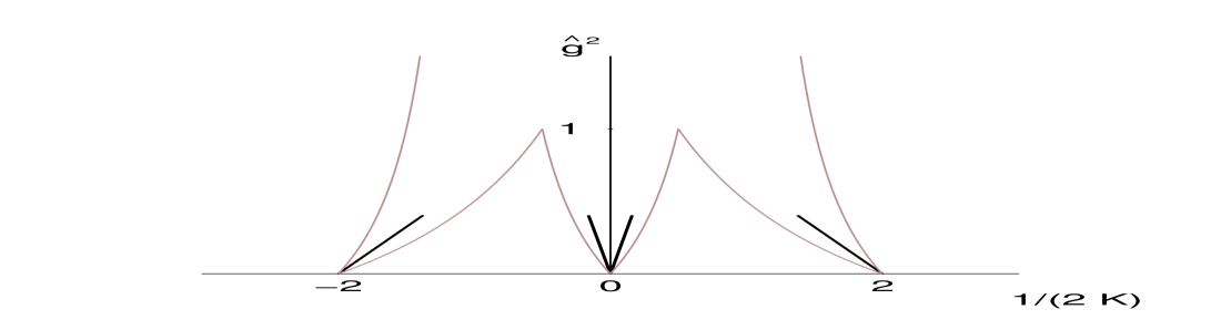
Figure 1: The phase diagram for the Gross-Neveu model in the weakly coupled region (to ${\cal{O}}(\hat{g}^{2})$) (dark lines) and a schematic representation of the expected Aoki phase diagram (light curves).

This weakly coupled phase diagram is pictured in Fig. 1 (dark lines). From left to right, the critical lines are traced out by the thermodynamic limits of the zeroes indexed by $(\hat{p}_{1},\hat{p}_{2})$ = $(\pm(N-1)/2,-N/2)$, $(\pm(N-1)/2,0)$, $(\pm 1/2,-N/2)$ and $(\pm 1/2,0)$ respectively. The lighter curves are a schematic representation of the expected full phase diagram.

In conclusion, we have developed a new type of weak coupling expansion which is multiplicative rather than additive in nature and focuses on the Lee-Yang zeroes, or protocritical points, of a lattice field theory with Wilson fermions. This expansion is applied to the Gross-Neveu model, where the existence of an Aoki phase was first suggested. The weakly coupled regime is the one of primary interest as it is there, as with all asymptotically free models, that the continuum limit is taken. The method, applied to the single flavour Gross-Neveu model, yields a phase diagram in this region which is consistent with that of Aoki and the widths of the Aoki cusps are determined to order ${\hat{g}}^{2}$.

Acknowledgements: RK wishes to thank M. Creutz for a discussion.

References

• [1] N. Kawamoto, Nucl. Phys. B 190 (1981) 617.
• [2] S. Aoki, Phys. Rev. D, 30 (1984) 2653; Nucl. Phys. B 314 (1989) 79.
• [3] T. Eguchi and R. Nakayama, Phys. Lett. B 126 (1983) 89.
• [4] S. Aoki and A. Gocksch, Phys. Lett. B 231 (1989) 449; ibid 243 (1990) 409; Phys. Rev D 45 (1992) 3845.
• [5] S. Aoki, A. Ukawa and T. Umemura, Phys. Rev. Lett. 76 (1996) 873; Nucl. Phys. B (Proc. Suppl.) 47 (1996) 511; S. Aoki, T. Kaneda, A. Ukawa and T. Umemura, Nucl. Phys. B (Proc. Suppl.) 453 (1997) 438; S. Aoki, T. Kaneda and A. Ukawa, Phys. Rev. D 56 (1997) 1808; S. Aoki, Nucl. Phys. B (Proc. Suppl.) 60A (1998) 206; K.M. Bitar, Nucl. Phys. B (Proc. Suppl.) 63 (1998) 829.
• [6] S. Sharpe and R.L. Singleton Jr., Phys. Rev. D 58 (1998) 074501; Nucl. Phys. B (Proc.Suppl.) 73 (1999) 234.
• [7] R. Kenna, C. Pinto and J.C. Sexton, e-Print Archive: hep-lat/9812004; Nucl. Phys. B (Proc. Suppl.) 83 (2000) 667.
• [8] K.M. Bitar, Phys. Rev. D 56 (1997) 2736; K.M. Bitar, U.M. Heller and R. Narayanan, Phys. Lett B 418 (1998) 167; R.G. Edwards, U.M. Heller, R. Narayanan and R.L. Singleton Jr., Nucl.Phys. B 518 (1998) 319.
• [9] H. Gausterer and C.B. Lang, Phys. Lett. B 341 (1994) 46; Nucl. Phys. B (Proc. Supl.) 34 (1994) 201; V. Azcoiti, G. Di Carlo, A. Galante, A.F. Grillo and V. Laliena, Phys. Rev. D 50 (1994) 6994; ibid. 53 (1996) 5069; I. Hip, C.B. Lang and R. Teppner, Nucl. Phys. B (Proc. Supl.) 63 (1998) 682.
• [10] M. Creutz, e-Print Archive: hep-lat/9608024 (Talk given at Brookhaven Theory Workshop on Relativistic Heavy Ions, Upton, NY, 8-19 Jul 1996); e-Print Archive: hep-lat/0007032.
• [11] S. Aoki, Prog. Theor. Phys. Suppl. 122 (1996) 179.
• [12] D.J. Gross and A. Neveu, Phys. Rev. D 10 (1974) 3235.
• [13] T.D. Lee and C.N. Yang, Phys. Rev. 87 (1952) 404; ibid. 410.
• [14] M.E. Fisher, Suppl. Prog. Theor. Phys. 69 (1980) 14.