Abstract

We study the renormalization of the $\Delta S=1$ effective weak Hamiltonian with overlap fermions. The mixing coefficients among dimension-six operators are computed at one loop in perturbation theory. As a consequence of the chiral symmetry at finite lattice spacing and of the GIM mechanism, which is quadratic in the masses, the $K\rightarrow\pi\pi$ and $K\rightarrow\pi$ matrix elements relevant for the $\Delta I=1/2$ rule can be computed without any power subtractions. The analogous amplitudes for $\epsilon^{\prime}/\epsilon$ require one divergent subtraction only, which can be performed non-perturbatively using $K\rightarrow 0$ matrix elements.

11.15.Ha, 12.38.Gc, 14.40.Aq

1 Introduction

The non-leptonic $\Delta S=1$ weak transitions are far from being understood. It is well known that the $\Delta I=1/2$ amplitudes are enhanced (the so-called $\Delta I=1/2$ rule) with respect to the corresponding $\Delta I=3/2$ ones (by roughly a factor $20$ in $K\rightarrow\pi\pi$ decays); the latest measurements of $\epsilon^{\prime}/\epsilon$ [1] confirm the rather large value found by NA31 [2], and the up-to-date world average is roughly $2\cdot 10^{-3}$. Given the present limited knowledge of the long-distance QCD effects in non-leptonic $\Delta S=1$ amplitudes, these experimental results cannot be predicted from first principles and well-controlled approximations.

The short-distance QCD corrections to the $\Delta S=1$ effective Hamiltonian can be reliably computed in perturbation theory [5]. In the Standard Model (SM) the Wilson coefficients are known up to the Next-to-Leading Order (NLO) [6, 7]. They account for a factor two of the enhancement in the $\Delta I=1/2$ rule and cannot reproduce the experimental value of $\epsilon^{\prime}/\epsilon$, when $\mbox{Im}\lambda_{t}\equiv V_{td}V^{*}_{ts}$ is determined from the unitarity triangle and the Vacuum Saturation Approximation (VSA) estimate of $\langle\pi\pi|O_{6}|K\rangle$ (see below) is used [8]-[10]. The SM could explain both effects if penguin contractions, neglected in the VSA, give contributions to the relevant matrix elements definitely larger than their factorized values [9]. Up to now no reliable first-principle computations of the $\Delta I=1/2$ matrix elements exist.

Lattice QCD is the only known method which allows one to compute non-perturbative QCD contributions to physical amplitudes from first principles. In the most popular lattice regularizations, i.e. Wilson and staggered fermions, the main theoretical aspects of the renormalization of composite operators are fully understood [11]-[13]. The results of quenched calculations of the matrix elements relevant for the $K^{0}$–$\bar{K}^{0}$ and $B^{0}$–$\bar{B}^{0}$ mixings have reached a high level of accuracy and are commonly used in phenomenological analyses of the unitarity triangle [14]-[17]. These lattice results have been crucial in constraining the parameters of the CKM matrix in the Standard Model (SM) [18, 9] and beyond [19]. Techniques to compute $\Delta I=1/2$ amplitudes for the $\Delta S=1$ Hamiltonian have been developed for both Wilson and staggered fermions [20, 21], but these methods have not yet produced useful results. There are two major difficulties:

• In Euclidean space there is apparently no simple relation between the two- (many-)body transition matrix elements and the corresponding correlation functions at large time separation [23]. This problem is common to all lattice discretizations and there are proposals to solve it either by using finite volume techniques [24] or studying the correlation functions in the large volume limit [25, 26];

• The operators we are interested in mix with lower-dimensional operators with coefficients which can diverge as inverse powers of the lattice spacing. These mixings can be more severe when chiral symmetry is broken by the regularization, like for Wilson fermions.

In the last few years it has been understood [27]-[29] that chiral and flavor symmetries can be preserved simultaneously on the lattice, without fermion doubling, if the fermionic operator $D$ satisfies the Ginsparg-Wilson Relation (GWR) [30]. This implies an exact invariance of the fermionic action which can be interpreted as a lattice realization of the standard chiral symmetry at finite cutoff [29]. However the GWR itself does not guarantee locality, the absence of doubler modes and the correct classical continuum limit.

Neuberger, through the overlap formalism [31], found a solution [27] of the GWR which satisfies all the above requirements and is local [32]. The complicated form of Neuberger’s operator renders its numerical implementation quite demanding for the present generation of computers. However, some progress has been achieved [33] and Monte Carlo simulations are already feasible, at least in the quenched approximation.

In this paper we study the renormalization of the $\Delta S=1$ effective weak Hamiltonian in the overlap regularization. Neuberger’s action implies many theoretical advantages:

• The quark masses renormalize only multiplicatively, the mixings among operators with different chirality are forbidden [28, 34] and their parity-violating and parity-conserving components renormalize in the same way [34];

• The GIM mechanism is as powerful as in the continuum to suppress mixing with lower-dimensional operators;

• The action and therefore the spectrum of the theory are free from $O(a)$ discretization errors. The $O(a)$ improvement of the local fermionic operators is greatly simplified [35].

As a consequence the $K\rightarrow\pi\pi$ and, if chiral perturbation theory ($\chi$PT) is used, $K\rightarrow\pi$ matrix elements for the $\Delta I=1/2$ rule can be computed without any power subtractions. The analogous matrix elements for $\epsilon^{\prime}/\epsilon$ require only one divergent subtraction which can be performed non-perturbatively using on-shell $K\rightarrow 0$ matrix elements. On the contrary, when the regularization breaks chiral symmetry the $K\rightarrow\pi$ matrix elements for the $\Delta I=1/2$ rule and for $\epsilon^{\prime}/\epsilon$ require one and two power-divergent subtractions respectively.

We also compute the mixing coefficients among dimension-six operators at one loop in perturbation theory. A further determination of these renormalization constants can be obtained using numerical non-perturbative methods such as those in Refs. [37, 38]. However a perturbative analysis is useful for analytically studying the mixing pattern of the operators, often gives accurate estimates of the renormalization constants and furnishes a consistency check of the non-perturbative methods.

The paper is organized as follows: in section 2 we define the $\Delta S=1$ effective Hamiltonian in the continuum; in sections 3 and 4 the overlap fermion action and the lattice $\Delta S=1$ operators are introduced, and in section 5 we compute at one loop the penguin diagrams of these operators. In sections 6 and 7 we describe the renormalization pattern of the relevant operators for the $\Delta I=1/2$ rule and $\epsilon^{\prime}/\epsilon$ and we report the main results of this paper; in section 8 we state our conclusions.

2 The $\Delta S=1$ effective Hamiltonian in the continuum

The $\Delta S=1$ effective Hamiltonian above the charm threshold is given by

$${\cal H}_{eff}^{\Delta S=1} = \lambda_{u}\frac{G_{F}}{\sqrt{2}}\Bigl{[}(1-\tau)\Bigl{(}C_{1}(\mu)\left(\widehat{Q}_{1}(\mu)-\widehat{Q}_{1}^{c}(\mu)\right)+C_{2}(\mu)\left(\widehat{Q}_{2}(\mu)-\widehat{Q}_{2}^{c}(\mu)\right)\Bigr{)}$$ (1)

$$+ \tau\sum_{i=1}^{10}C_{i}(\mu)\widehat{Q}_{i}(\mu)\Bigr{]}\;,$$

where $G_{F}$ is the Fermi coupling constant, $\tau=-\lambda_{t}/\lambda_{u}$, $\lambda_{u}=V_{ud}V^{*}_{us}$, $\lambda_{t}=V_{td}V^{*}_{ts}$ and $\mu$ is the renormalization scale of the composite operators. The Wilson coefficients $C_{i}(\mu)$ at the NLO in QCD and QED have been given in [6, 7]. The operator basis is

$$Q_{1} = ({\bar{s}}^{\alpha}\gamma^{\mu}_{L}u^{\beta})({\bar{u}}^{\beta}\gamma^{\mu}_{L}d^{\alpha})$$

$$Q_{2} = ({\bar{s}}\gamma^{\mu}_{L}u)({\bar{u}}\gamma^{\mu}_{L}d)$$

$$Q_{3,5} = ({\bar{s}}\gamma^{\mu}_{L}d)\sum_{q}({\bar{q}}\gamma^{\mu}_{L,R}q)$$

$$Q_{4,6} = ({\bar{s}}^{\alpha}\gamma^{\mu}_{L}d^{\beta})\sum_{q}({\bar{q}}^{\beta}\gamma^{\mu}_{L,R}q^{\alpha})$$

$$Q_{7,9} = \frac{3}{2}({\bar{s}}\gamma^{\mu}_{L}d)\sum_{q}e_{q}({\bar{q}}\gamma^{\mu}_{R,L}q)$$

$$Q_{8,10} = \frac{3}{2}({\bar{s}}^{\alpha}\gamma^{\mu}_{L}d^{\beta})\sum_{q}e_{q}({\bar{q}}^{\beta}\gamma^{\mu}_{R,L}q^{\alpha})$$

$$Q^{c}_{1} = ({\bar{s}}^{\alpha}\gamma^{\mu}_{L}c^{\beta})({\bar{c}}^{\beta}\gamma^{\mu}_{L}d^{\alpha})$$

$$Q^{c}_{2} = ({\bar{s}}\gamma^{\mu}_{L}c)({\bar{c}}\gamma^{\mu}_{L}d)\;,$$ (2)

where $\gamma^{\mu}_{L,R}=\gamma^{\mu}(1\mp\gamma_{5})$, $e_{q}$ are the quark electric charges and $\alpha,\beta$ denote color indices (which are omitted for the color-singlet operators). Below the bottom threshold, $q$ runs over the active flavors $u,d,s,c$. Other operators would appear in Eq. (1), but in the Standard Model they are numerically irrelevant and they will not be considered in this paper.

The electro-penguin operators $Q_{i}$ ($i=7,\dots,10$) give significant contributions to $\epsilon^{\prime}/\epsilon$ only through their $\Delta I=3/2$ components. In the limit $m_{u}=m_{d}$, $Q^{3/2}_{i}$ do not mix with lower-dimensional operators and their renormalization constants in the overlap regularization can be obtained from [34]. Therefore in the following we will focus only on the computations of the matrix elements of $Q_{1},\dots,Q_{6}$ (and $Q^{c}_{1},Q^{c}_{2}$).

Under flavor $SU(3)_{L}\times SU(3)_{R}$ transformations, the combination

$$Q_{27}=2Q_{2}+3Q_{1}-Q_{3}+Q^{c}_{1}$$ (3)

transforms as a $(27_{L},1_{R})$ multiplet and induces both $\Delta I=1/2$ and $\Delta I=3/2$ transitions. The operators

$$Q_{-}=Q_{1}-Q_{2}$$ (4)

and $Q_{i}$ ($i=3,4,5,6$) transform as $(8_{L},1_{R})$ operators and induce pure $\Delta I=1/2$ transitions.

The octet operators are linearly dependent; by performing Fierz transformations it is easy to show that

$$Q_{4}=Q_{3}+Q_{2}-Q_{1}+Q_{2}^{c}-Q_{1}^{c}\;.$$ (5)

For $\mu<m_{c}$ the operator basis is given by $Q_{1}-Q_{10}$ and the sums over $q$ in the penguin operators run over $u,d,s$ only. The relation (5) becomes

$$Q_{4}=Q_{3}+Q_{2}-Q_{1}$$ (6)

and in Eq. (3) $Q^{c}_{1}$ has to be dropped.

3 Basic definitions for overlap fermions

The QCD lattice action we consider for massive fermions is

$$S_{L}=\frac{6}{g_{0}^{2}}\sum_{P}\bigg{[}1-\frac{1}{6}\mbox{Tr}\;\Big{[}U_{P}+U_{P}^{\dagger}\Big{]}\bigg{]}+\bar{q}\left[\Big{(}1-\frac{1}{2\rho}am_{q}\Big{)}D_{N}+m_{q}\right]\,q,$$ (7)

where, in standard notation, $U_{P}$ is the Wilson plaquette, $g_{0}$ is the bare coupling constant and $m_{q}$ is the bare fermion mass. $D_{N}$ is the Neuberger-Dirac operator defined as

$$D_{N} = \frac{\rho}{a}\left(1+X\frac{1}{\sqrt{X^{\dagger}X}}\right)$$

$$X = D_{W}-\frac{1}{a}\rho\;,$$ (8)

where

$$D_{W}=\frac{1}{2}\gamma_{\mu}(\nabla_{\mu}+\nabla^{*}_{\mu})-\frac{r}{2}a\nabla^{*}_{\mu}\nabla_{\mu}$$ (9)

is the Wilson-Dirac operator, $0<r\leq 1$ and $0<\rho<2r$. $\nabla_{\mu}$ and $\nabla^{*}_{\mu}$ are the forward and backward lattice derivatives, i.e.

$$\nabla_{\mu}q(x) = \frac{1}{a}\Big{[}U_{\mu}(x)q(x+a\hat{\mu})-q(x)\Big{]}$$

$$\nabla_{\mu}^{*}q(x) = \frac{1}{a}\Big{[}q(x)-U^{\dagger}_{\mu}(x-a\hat{\mu})q(x-a\hat{\mu})\Big{]}\;,$$ (10)

where $U_{\mu}(x)$ are the lattice gauge links.

The overlap-Dirac operator satisfies the Ginsparg-Wilson relation

$$\gamma_{5}D_{N}+D_{N}\gamma_{5}=\frac{a}{\rho}D_{N}\gamma_{5}D_{N}$$ (11)

which, in the massless limit, implies a continuous symmetry of the action which may be interpreted as a lattice form of the chiral invariance [29]:

$$\delta q=\hat{\gamma}_{5}q\;,\qquad\delta\bar{q}=\bar{q}\gamma_{5}\;,$$ (12)

where $\hat{\gamma}_{5}$ is defined as

$$\hat{\gamma}_{5}=\gamma_{5}\Big{(}1-\frac{a}{\rho}D_{N}\Big{)}$$ (13)

and satisfies

$$\hat{\gamma}_{5}^{\dagger}=\hat{\gamma}_{5}\;,\qquad\hat{\gamma}_{5}^{2}=1\;.$$ (14)

If we define the chiral projectors as

$$\hat{P}_{\pm}=\frac{1}{2}(1\pm\hat{\gamma}_{5})\;,\qquad P_{\pm}=\frac{1}{2}(1\pm\gamma_{5})\;,$$ (15)

the fermionic fields can be decomposed into left- and right-handed components [3, 40, 41]

$$q_{R,L}=\hat{P}_{\pm}q\qquad\bar{q}_{R,L}=\bar{q}P_{\mp}$$ (16)

which transform under lattice chiral rotations in the same way as the corresponding fields in the continuum. The massive fermion matrix in Eq. (7) can be written as

$$D_{N}(m)=P_{+}D_{N}\hat{P}_{-}+P_{-}D_{N}\hat{P}_{+}+m(P_{-}\hat{P}_{-}+P_{+}\hat{P}_{+})\;.$$ (17)

The composite fermionic operators can be defined to have the same combination of left and right components as in the continuum. This guarantees that under lattice chiral rotations they transform as the corresponding operators in the continuum. As an example, the bilinear operators can be defined as

$${\cal O}_{\Gamma}=\bar{q}_{1}\bar{\Gamma}q_{2}\;,$$ (18)

where $\bar{\Gamma}=\Gamma(1-\frac{a}{2\rho}D_{N})$. The on-shell matrix elements of these operators are $O(a)$ improved [35]. The Feynman rules corresponding to the action in Eq. (7) are given in [34] and are in agreement with those used in [42]-[44]. Reference [34] also gives in detail all conventions and symbols used in this paper.

4 $\Delta S=1$ four-fermion operators on the lattice

The four-flavor QCD lattice action in the overlap regularization reads

$$S=\frac{6}{g_{0}^{2}}\sum_{P}\bigg{[}1-\frac{1}{6}\mbox{Tr}\;\Big{[}U_{P}+U_{P}^{\dagger}\Big{]}\bigg{]}+\sum_{q}\bar{q}\left[\Big{(}1-\frac{1}{2\rho}am_{q}\Big{)}D_{N}+m_{q}\right]\,q,$$ (19)

where $q=u,d,s,c$. In the limit $m_{u}=m_{d}=m_{s}=0$, this action is invariant under the $SU(3)_{L}\times SU(3)_{R}$ group and the corresponding transformations are defined as

$$\psi_{L}\rightarrow U\psi_{L}\;, \bar{\psi}_{L}\rightarrow\bar{\psi}_{L}U^{\dagger}$$

$$\psi_{R}\rightarrow V\psi_{R}\;, \bar{\psi}_{R}\rightarrow\bar{\psi}_{R}V^{\dagger}\;,$$ (20)

where $\psi_{L,R}=(u_{L,R},d_{L,R},s_{L,R})$ is a column vector in flavor space and

$$U^{\dagger}U = V^{\dagger}V=\hbox{1$\!\!$1}$$

$$\mbox{det}U = \mbox{det}V=1\;.$$ (21)

When $u,d,s$ acquire a mass, the action is invariant if the light quark masses are transformed as

$$M=\left(\begin{array}[]{ccc}m_{u}&&\\ &m_{d}&\\ &&m_{s}\\ \end{array}\right)\rightarrow UMV^{\dagger}\;.$$ (22)

A convenient definition for the lattice four-fermion operators of the $\Delta S=1$ effective Hamiltonian is

$${\cal Q}_{1} = ({\bar{s}}^{\alpha}\bar{\gamma}^{\mu}_{L}u^{\beta})({\bar{u}}^{\beta}\bar{\gamma}^{\mu}_{L}d^{\alpha})$$

$${\cal Q}_{2} = ({\bar{s}}\bar{\gamma}^{\mu}_{L}u)({\bar{u}}\bar{\gamma}^{\mu}_{L}d)$$

$${\cal Q}_{3,5} = ({\bar{s}}\bar{\gamma}^{\mu}_{L}d)\sum_{q}({\bar{q}}\bar{\gamma}^{\mu}_{L,R}q)$$ (23)

$${\cal Q}_{4,6} = ({\bar{s}}^{\alpha}\bar{\gamma}^{\mu}_{L}d^{\beta})\sum_{q}({\bar{q}}^{\beta}\bar{\gamma}^{\mu}_{L,R}q^{\alpha})$$

$${\cal Q}^{c}_{1} = ({\bar{s}}^{\alpha}\bar{\gamma}^{\mu}_{L}c^{\beta})({\bar{c}}^{\beta}\bar{\gamma}^{\mu}_{L}d^{\alpha})$$

$${\cal Q}^{c}_{2} = ({\bar{s}}\bar{\gamma}^{\mu}_{L}c)({\bar{c}}\bar{\gamma}^{\mu}_{L}d)\;,$$

where $\bar{\gamma}^{\mu}_{L,R}=\gamma^{\mu}_{L,R}(1-\frac{a}{2\rho}D_{N})$. Under the rotations in Eq. (4), these operators transform as the analogous operators in the continuum and their on-shell matrix elements are $O(a)$ improved.

Under renormalization the operators in Eqs. (4) can mix with equal- or lower-dimensional operators which have the same transformation properties under $SU(3)_{L}\times SU(3)_{R}$ or, due to the explicit soft chiral symmetry-breaking term, with multiplets of different chirality properly multiplied by light quark masses. As in the continuum, ${\cal Q}_{27}$ is multiplicatively renormalizable while the $(8_{L},1_{R})$ operators can mix among themselves as well as with two lower-dimensional operators [21, 45] (besides operators which vanish by the equations of motion)

$${\cal Q}_{\sigma} = g_{0}\left[(m_{s}+m_{d})\bar{s}\bar{\sigma}_{\mu\nu}F_{\mu\nu}d+(m_{s}-m_{d})\bar{s}\bar{\sigma}_{\mu\nu}\widetilde{F}_{\mu\nu}d\right]$$ (24)

$${\cal Q}_{m} = (m_{s}+m_{d})\bar{s}\bar{\hbox{1$\!\!$1}}d+(m_{s}-m_{d})\bar{s}\bar{\gamma}_{5}d\;,$$ (25)

where $F_{\mu\nu}$ and $\widetilde{F}_{\mu\nu}$ are the non-abelian gluon field tensor and its dual, $\bar{\sigma}_{\mu\nu}=\sigma_{\mu\nu}(1-\frac{a}{2\rho}D_{N})$, $\bar{\gamma}_{5}=\gamma_{5}(1-\frac{a}{2\rho}D_{N})$ and $\bar{\hbox{1$\!\!$1}}=(1-\frac{a}{2\rho}D_{N})$. The definition of the properly subtracted operators necessary for the $\Delta I=1/2$ rule and for $\epsilon^{\prime}/\epsilon$ will be given in sections 6 and 7.

5 Penguin diagrams in perturbation theory

In this section we discuss the calculation of the penguin diagrams at one loop in perturbation theory. The four-point Green’s functions of a four-fermion operator between quark states are defined as

$$G_{i}(x_{1},x_{2},x_{3},x_{4})=\langle q_{1}(x_{1})\bar{q}_{2}(x_{2})Q_{i}(0)q_{3}(x_{3})\bar{q}_{4}(x_{4})\rangle\,,$$ (26)

where $x_{1},x_{3}$ and $x_{2},x_{4}$ are the coordinates of the outgoing and incoming quarks respectively. Note that $G_{i}$ depends implicitly on the color and Dirac indices carried by the external fermion fields. The Fourier transform of the Green’s functions (26), with external momenta $p$ and $p^{\prime}$ chosen as in Figs. 1 and 2, is defined as

$$G_{i}(p,p^{\prime})=\int dx_{1}dx_{2}dx_{3}dx_{4}e^{-ip(x_{1}-x_{4})}e^{-ip^{\prime}(x_{3}-x_{2})}G_{i}(x_{1},x_{2},x_{3},x_{4})\;.$$ (27)

The corresponding amputated correlation functions are defined as

$$\Lambda_{i}(p,p^{\prime})=S^{-1}(p)S^{-1}(p^{\prime})G_{i}(p,p^{\prime})S^{-1}(p^{\prime})S^{-1}(p)\;,$$ (28)

where $S(p)$ denotes the quark propagator in momentum space. At one loop, the only diagrams which contribute to the mixing among dimension-six operators are the penguin diagrams in Fig. 1 and the vertex diagrams in Fig. 2. As for the $\Delta F=2$ operators in Ref. [34], it can be proven that the operators in Eqs. (4) renormalize as the corresponding local ones. Therefore in the following all one-loop computations are performed with local operators.

The vertex diagrams in Fig. 2 have been computed in Ref. [34]; they are sufficient for the renormalization of the $\Delta F=2$ operators and do not give rise to mixing with lower-dimensional operators. The penguin diagrams in Fig. 1 are computed here for the first time and constitute one of the main results of this paper.

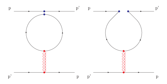
Figure 1: Penguin diagrams for four-fermion operators.

The calculations involve the gauge-invariant quantity

$${\cal P}_{\mu}(ak,am)=\int_{-\pi/a}^{\pi/a}\frac{d^{4}l}{(2\pi)^{4}}S^{(0)}_{N}(l-\frac{k}{2})V^{(1)}_{\mu}(l+\frac{k}{2},l-\frac{k}{2})S^{(0)}_{N}(l+\frac{k}{2})\;,\qquad k=p^{\prime}-p\;,$$ (29)

which does not depend on the flavor, spin and color structures of the operators, and is the result of the internal quark loop once these structures have been factored out. The tree-level overlap propagator $S^{(0)}_{N}(p)$ and the quark-gluon vertex $V^{(1)}_{\mu}(p,p^{\prime})$ are defined in Ref. [34]. Eventually we will impose the RI renormalization scheme and therefore we can perform all the computations in the massless limit. ${\cal P}_{\mu}(ak,0)$ has to be computed by expanding vertices and propagators to second order in $ak$, since in the diagrams in Fig. 1 it is contracted with the gluon propagator $G(ak)\sim(ak)^{-2}$.

For the analytic computations we have used FORM codes which we have developed specifically for this problem; the output has been integrated on a $60^{4}$ grid. Among other checks, we have computed ${\cal P}_{\mu}(ak,0)$ using different assignments for the loop momenta. We also checked that the spectator quark line contributes only with its continuum expression. The result for overlap fermions is

$${\cal P}_{\mu}(ak,0)=i\frac{g_{0}}{16\pi^{2}}\Bigg{[}-\frac{1}{3}\log a^{2}k^{2}+B_{peng}\Bigg{]}\Big{(}\gamma_{\mu}k^{2}-k\!\!\!/k_{\mu}\Big{)},$$ (30)

where $B_{peng}$ is given in Table 1 for several values of $\rho$. Notice the structure in $k$ which comes from gauge invariance.

$\rho$	$B_{\psi}$	$B_{S}$	$B_{V}$	$B_{peng}$
0.2	-235.80762	1.31942	1.52122	0.64996
0.3	-150.61868	1.89625	1.52277	0.49361
0.4	-108.19798	2.38060	1.52448	0.45000
0.5	-82.86081	2.80522	1.52637	0.44558
0.6	-66.05227	3.18782	1.52845	0.45796
0.7	-54.10921	3.53927	1.53074	0.47845
0.8	-45.20179	3.86686	1.53329	0.50317
0.9	-38.31447	4.17577	1.53611	0.53024
1.0	-32.83862	4.46989	1.53924	0.55875
1.1	-28.38734	4.75224	1.54274	0.58826
1.2	-24.70304	5.02527	1.54665	0.61863
1.3	-21.60760	5.29104	1.55105	0.64992
1.4	-18.97397	5.55135	1.55601	0.68235
1.5	-16.70910	5.80783	1.56163	0.71635
1.6	-14.74330	6.06201	1.56804	0.75261
1.7	-13.02336	6.31544	1.57541	0.79229
1.8	-11.50798	6.56970	1.58394	0.83759

Table 1: Perturbative values of the finite parts of the amputated correlation functions in the Landau gauge for the self energy, the scalar density and the vector current. The gauge-invariant penguin constant $B_{peng}$ defined in Eq. (30) is reported in the last column.

The $k\!\!\!/$ term vanishes, up to $O(g_{0}^{2})$, if the equations of motion are used for the spectator quarks [46], and the $k^{2}$ in the remaining structure $\gamma_{\mu}k^{2}$ disappears when combined with the gluon propagator.

We have used our codes to compute the penguin diagrams also in the Wilson case,

$${\cal P}^{W}_{\mu}(ak,0) = i\frac{g_{0}}{16\pi^{2}}\Bigg{[}-\frac{1}{3}\log a^{2}k^{2}+0.5709352\Bigg{]}\Big{(}\gamma_{\mu}k^{2}-k\!\!\!/k_{\mu}\Big{)}$$

$$= i\frac{g_{0}}{16\pi^{2}}\Bigg{[}-\frac{1}{3}\log\frac{a^{2}k^{2}}{\pi^{2}}-0.1922181\Bigg{]}\Big{(}\gamma_{\mu}k^{2}-k\!\!\!/k_{\mu}\Big{)},$$

and we are in agreement with the results by Bernard et al. [46]. It is interesting to note that the overlap result for $\rho=1$ is not too far from the Wilson number. In the Wilson case the lack of chiral symmetry causes, even in the massless case, the presence in ${\cal P}^{W}_{\mu}(ak,0)$ of an additional power-divergent term which contains tensor operators:

$$-0.39847257\,\frac{1}{a}\frac{g_{0}}{16\pi^{2}}\sigma_{\mu\lambda}k_{\lambda}.$$ (32)

We have also observed that, as expected, for overlap fermions the coefficient of the tensor term is zero (within our integration precision). This constitutes another test of the numerical accuracy of our integrals.

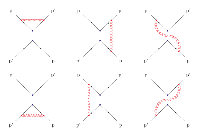
Figure 2: Feynman graphs for the vertex corrections to four-fermion operators.

A generic local four-fermion operator can give rise to one or more of the following penguin types:

$$P_{A1} = (\bar{s}\Gamma{\cal T}q)(\bar{q}\Gamma^{\prime}{\cal T}^{\prime}d)$$

$$P_{A2} = (\bar{s}^{\alpha}\Gamma q^{\beta})(\bar{q}^{\beta}\Gamma^{\prime}d^{\alpha})$$

$$P_{B1} = (\bar{s}\Gamma{\cal T}d)(\bar{q}\Gamma^{\prime}{\cal T}^{\prime}q)$$ (33)

$$P_{B2} = (\bar{s}^{\alpha}\Gamma d^{\beta})(\bar{q}^{\beta}\Gamma^{\prime}q^{\alpha}).$$

The Wick contractions which form the quark loop are always meant to be only between $q$ and $\bar{q}$, and at one loop they give

$$\begin{array}[]{ccccc}{\cal I}_{A1}=-ig_{0}G(ak)(\bar{s}\Gamma&{\cal P}_{\mu}(ak,am)\Gamma^{\prime}&{\cal T}t^{A}{\cal T^{\prime}}&d)(\bar{f}t^{A}\gamma_{\mu}f)&\\ {\cal I}_{A2}=-ig_{0}G(ak)(\bar{s}\Gamma&{\cal P}_{\mu}(ak,am)\Gamma^{\prime}&\mbox{tr}(t^{A})&d)(\bar{f}t^{A}\gamma_{\mu}f)&=0\\ {\cal I}_{B1}=-ig_{0}G(ak)(\bar{s}\Gamma&\mbox{tr}(-{\cal P}_{\mu}(ak,am)\Gamma^{\prime})&{\cal T}\mbox{tr}(t^{A}{\cal T^{\prime}})&d)(\bar{f}t^{A}\gamma_{\mu}f)&\\ {\cal I}_{B2}=-ig_{0}G(ak)(\bar{s}\Gamma&\mbox{tr}(-{\cal P}_{\mu}(ak,am)\Gamma^{\prime})&t^{A}&d)(\bar{f}t^{A}\gamma_{\mu}f)&,\end{array}$$ (34)

where $G(ak)$ is the gluon propagator given in Ref. [34] and $f$ is the spectator quark. For the contractions $P_{A1}$ and $P_{A2}$ the relevant diagram is the one on the right of Fig. 1, while for $P_{B1}$ and $P_{B2}$ it is the diagram on the left. Weak operators in which $q=d$ or $q=s$, since they have three quarks of the same flavor, can undergo two Wick contractions instead of only one, therefore contributing with both diagrams to their renormalization factors.

The 1-loop penguin corresponding to ${\cal I}_{A2}$ is zero because of the tracelessness of the $t^{A}$ matrices; when ${\cal T}={\cal T}^{\prime}=\hbox{1$\!\!$1}$ the penguin contribution ${\cal I}_{B1}$ also vanishes for the same reason. Notice also that, since ${\cal P}_{\mu}$ enters in the expressions (34) either as $\Gamma{\cal P}_{\mu}\Gamma^{\prime}$ or as $\Gamma\mbox{tr}(-{\cal P}_{\mu}\Gamma^{\prime})$, the contribution of the $\sigma_{\mu\lambda}$ term of Eq. (32) in the Wilson case vanishes for all operators considered in this paper.

6 Renormalization pattern for the $\Delta I=1/2$ rule

For renormalization scales above the charm mass the bulk of the CP-conserving $\Delta I=1/2$ amplitudes comes from the operators

$${\cal O}_{\pm}=({\cal Q}_{1}-{\cal Q}^{c}_{1})\pm({\cal Q}_{2}-{\cal Q}^{c}_{2})\;.$$ (35)

The contributions which arise when the top quark is integrated out are suppressed by a factor $\lambda_{t}/\lambda_{u}$ and can be neglected.

Chiral symmetry forbids mixings with other dimension-six operators and the flavor structure forbids mixings between ${\cal O}_{+}$ and ${\cal O}_{-}$. When chiral symmetry is preserved, the GIM mechanism ensures that the mixing with ${\cal Q}_{\sigma}$ and ${\cal Q}_{m}$ (Eqs. (24) and (25)) vanishes as $m_{c}^{2}-m_{u}^{2}$ when $m_{c}\rightarrow m_{u}$. This can be shown as in the continuum: the penguin contractions of left-left four-fermion operators take non-vanishing contributions only when the helicity, which is preserved through the massless quark lines, is flipped by an even number of mass insertions. Therefore in the overlap regularization the renormalized operators read as

$$\widehat{O}_{\pm}(\mu) = Z_{\pm}(\mu a,g^{2}_{0})\widetilde{\cal O}_{\pm}(a)+O(a^{2})$$ (36)

$$\widetilde{\cal O}_{\pm}(a) = {\cal O}_{\pm}(a)+(m^{2}_{c}-m^{2}_{u})C_{\pm}^{m}(g_{0}^{2}){\cal Q}_{m}(a)\;,$$

where $Z_{\pm}(\mu a,g^{2}_{0})$ are $O(1)$ logarithmic divergent renormalization constants, $C_{\pm}^{m}(g_{0}^{2})$ are finite mixing coefficients [47] which are suppressed by a factor $\alpha_{s}$ and the contributions proportional to ${\cal Q}_{\sigma}$ give $O(a^{2})$ effects. $Z_{\pm}$ and $C_{\pm}^{m}$ can be determined by imposing two renormalization conditions which, in perturbation theory, would specify their two- and four-quark amputated Green’s functions.

For $Z_{\pm}$ we opt for the RI renormalization scheme proposed in [37, 48]. $Z^{\mbox{\scriptsize RI}}_{\pm}$ are defined by imposing that the renormalized amputated Green’s functions at large fixed Euclidean scale $\mu^{2}$, in the Landau gauge and in the massless limit, are equal to their tree-level values, i.e.

$$Z^{\mbox{\scriptsize RI}}_{\pm}(\mu a,g^{2}_{0})\Lambda_{\pm}(p,p^{\prime})\Big{|}_{p^{2}={p^{{}^{\prime}2}}=\mu^{2}}=\Lambda_{\pm}^{(0)}(p,p^{\prime})\Big{|}_{p^{2}={p^{{}^{\prime}2}}=\mu^{2}}\;.$$ (37)

At one loop the relevant contributions to $Z^{\mbox{\scriptsize RI}}_{\pm}$ come from the vertex diagrams in Fig. 2, while the penguin diagrams cancel in the massless limit due to the GIM mechanism. Using the results in Ref. [34] we obtain

$$Z_{\pm}^{\mbox{\scriptsize RI}}=1-\frac{g_{0}^{2}}{16\pi^{2}}\left[\frac{\gamma^{(0)}_{\pm}}{2}\log(\mu^{2}a^{2})+B_{\pm}+2\frac{N_{c}^{2}-1}{2N_{c}}B_{\psi}\right]\;,$$ (38)

where

$$\gamma^{(0)}_{+}=4 B_{+}=\frac{10}{3}B_{V}-\frac{2}{3}B_{S}$$

$$\gamma^{(0)}_{-}=-8 B_{-}=\frac{4}{3}(B_{S}+B_{V})\;.$$ (39)

The constants $B_{\psi}$, $B_{S}$ and $B_{V}$, which enter the renormalization of the quark propagator, the scalar density and the vector current, were computed in [43, 34] for several values of $\rho$ and are reported in Table 1 for completeness. The anomalous dimensions $\gamma^{(0)}_{\pm}$ are in agreement with those in Refs. [6, 7] and the matching coefficients between RI and one of the $\overline{\mbox{MS}}$ schemes can be found in [48].

The mixing coefficients $C^{(\pm)}_{m}$ can be determined by imposing suitable renormalization conditions on two-quark correlation functions computed at two loops in perturbation theory. As in the continuum, these coefficients are not needed for the physical $K\rightarrow\pi\pi$ matrix elements. For $K\rightarrow\pi$ amplitudes we will show that they can be fixed non-perturbatively by imposing suitable renormalization conditions on the $K\rightarrow 0$ matrix elements.

The $K\rightarrow\pi\pi$ matrix elements

$$\langle\pi\pi|\widehat{O}_{\pm}(\mu)|K\rangle=Z_{\pm}(\mu a,g^{2}_{0})\langle\pi\pi|\left[{\cal O}_{\pm}(a)+(m^{2}_{c}-m^{2}_{u})C_{\pm}^{m}(g_{0}^{2}){\cal Q}_{m}(a)\right]|K\rangle\;$$ (40)

can be extracted directly from the four-point functions once the final state interactions have been properly taken into account [24]-[26]. Following [49], the on-shell matrix elements of the pseudoscalar density ${\cal P}=\bar{s}\bar{\gamma}_{5}d$ satisfies the Axial Ward Identity

$$Z_{A}\langle\pi\pi|\partial_{\mu}{\cal A}_{\mu}|K\rangle=(m_{s}+m_{d})\langle\pi\pi|{\cal P}|K\rangle+O(a^{2})\;,$$ (41)

where ${\cal A}_{\mu}=\bar{s}\gamma_{\mu}\bar{\gamma}_{5}d$ and $Z_{A}$ is its renormalization constant, and up to $O(a^{2})$ effects $\langle\pi\pi|{\cal P}|K\rangle$ vanishes when the momentum $\Delta p$ inserted by the operator is zero. Eventually the physical matrix elements in the RI scheme read

$$\langle\pi\pi|\widehat{O}_{\pm}(\mu)|K\rangle=Z^{\mbox{\scriptsize RI}}_{\pm}(\mu a,g^{2}_{0})\langle\pi\pi|{\cal O}_{\pm}(a)|K\rangle+O(a^{2})\;.$$ (42)

Even if the momentum inserted is not zero, the contribution proportional to $\Delta p$ is finite and suppressed by a factor $\alpha_{s}$. Therefore the extrapolation to the physical point $\Delta p=0$ would not be a problem. The direct computation described above does not rely on chiral perturbation theory and in principle the use of $O(a)$ improved operators renders the computation of the matrix elements sensitive to higher-order chiral contributions. The two main advantages of the overlap regularization with respect to the Wilson fermions are that the mixings with dimension-three operators are finite even at non-zero momentum transfer ($\Delta p\neq 0$) and the improvement of the bilinear and four-fermion operators can be performed without tuning any parameters. The main difficulties of this method are that the final state interactions have to be taken properly into account and the computations of the four-point functions are technically quite complicated which could lead to noisy signals.

These difficulties can be avoided if one applies the method proposed in [20, 21], where it has been suggested to use chiral perturbation theory to relate $K\rightarrow\pi\pi$ to $K\rightarrow\pi$ matrix elements and to compute the latter on the lattice. At the leading order in $\chi$PT

$$\langle 0|{\cal O}_{\pm}|K^{0}\rangle = i\delta_{\pm}(m_{K}^{2}-m_{\pi}^{2})$$ (43)

$$\langle\pi^{+}(p)|{\cal O}_{\pm}|K^{+}(q)\rangle = \alpha_{\pm}\;p\cdot q\;-\delta_{\pm}\frac{m_{K}^{2}}{f_{\pi}}\;,$$ (44)

$$\langle\pi^{+}\pi^{-}|{\cal O}_{\pm}|K^{0}\rangle = i\alpha_{\pm}\frac{m_{K}^{2}-m_{\pi}^{2}}{f_{\pi}}\;,$$ (45)

and $\alpha_{\pm}$ can be computed by extracting $\langle\pi^{+}(p)|{\cal O}_{\pm}|K^{+}(q)\rangle$ from the three-point functions and fitting the results as a function of $p\cdot q$ and $m_{K}^{2}$. The unphysical contribution proportional to $\delta_{\pm}$ is not divergent. This is one of the main results of this paper. $\delta_{\pm}$ can also be subtracted by fixing $C_{\pm}^{m}$ in such a way that [45]

$$\langle 0|\widetilde{O}_{\pm}|K^{0}\rangle=0\;,$$ (46)

i.e.

$$C_{\pm}^{m}=-\frac{\delta_{\pm}}{\delta_{p}(m_{c}^{2}-m_{u}^{2})}\frac{m_{K}^{2}-m_{\pi}^{2}}{m_{s}-m_{d}}$$ (47)

with

$$\langle 0|{\cal P}|K^{0}\rangle=i\delta_{p}\;.$$ (48)

The comparison of the two methods is a check of the whole procedure. Since only single-particle states are involved there are no problems with final state interactions and the three-point functions are technically easier to simulate.

From the considerations reported above, we can appreciate the advantages of using Neuberger’s fermions to compute the matrix elements necessary for the $\Delta I=1/2$ rule:

• the GIM mechanism combined with chiral symmetry constrains the mixing coefficients with lower-dimensional operators to be proportional to $m_{c}^{2}-m_{u}^{2}$;

• the mixing coefficients with parity-conserving and parity-violating components of lower-dimensional operators are the same and are multiplied by $m_{s}-m_{d}$ and $m_{s}+m_{d}$ respectively;

• ${\cal O}^{\pm}(a)$ do not mix with dimension-six operators with different chiralities;

• the $O(a)$ improvement of the operators does not require any tuning of parameters.

On the contrary, in the Wilson regularization the parity-conserving components of ${\cal O}^{\pm}$ can mix with dimension-six operators of different chiralities, their mixing with lower-dimensional operators is no longer proportional to $m_{s}+m_{d}$ and the GIM mechanism gives only a factor $m_{c}-m_{u}$. Therefore the contributions of the chromomagnetic operator have to be subtracted and the scalar operator mixes with quadratically divergent coefficients. Finally for Wilson fermions the $O(a)$ improvement of the four-fermion composite operators requires tuning many parameters.

7 Renormalization pattern for $\epsilon^{\prime}/\epsilon$

For CP violating processes in kaon decays, when the top quark is integrated out, the GIM mechanism is not operative and the presence or not of an active charm does not substantially modify the mixing pattern of the relevant operators. Therefore, in this section we will consider the case with the charm quark integrated out. The corresponding $\Delta S=1$ effective Hamiltonian can be obtained from Eq. (1) and is reported, for example, in Ref. [6].

Analogously to the continuum, the operator

$${\cal Q}_{27}=2{\cal Q}_{2}+3{\cal Q}_{1}-{\cal Q}_{3}$$ (49)

does not mix with lower-dimensional operators and it is multiplicatively renormalizable:

$$\widehat{Q}_{27}(\mu)=Z_{27}(\mu a,g^{2}_{0}){\cal Q}_{27}(a)\;.$$ (50)

At one loop in perturbation theory only the diagrams in Fig. 2 give contributions to $Z_{27}(\mu a,g^{2}_{0})$ and in the RI scheme, defined analogously to Eq. (37), we obtain

$$Z^{\mbox{\scriptsize RI}}_{27}(\mu a)=1-\frac{g_{0}^{2}}{16\pi^{2}}\left[\frac{\gamma^{(0)}_{27}}{2}\log(\mu^{2}a^{2})+B_{27}+2\frac{N_{c}^{2}-1}{2N_{c}}B_{\psi}\right]\;,$$ (51)

with

$$\gamma^{(0)}_{27}=4\qquad B_{27}=\frac{10}{3}B_{V}-\frac{2}{3}B_{S}\;.$$ (52)

Also in this case chiral perturbation theory can be used to relate $K\rightarrow\pi\pi$ to $K\rightarrow\pi$ matrix elements and the latter can be extracted from the three-point functions computed numerically.

The mixing pattern of the QCD penguin operators

$${\cal Q}_{3,5} = ({\bar{s}}\bar{\gamma}^{\mu}_{L}d)\sum_{q}({\bar{q}}\bar{\gamma}^{\mu}_{L,R}q)$$ (53)

$${\cal Q}_{4,6} = ({\bar{s}}^{\alpha}\bar{\gamma}^{\mu}_{L}d^{\beta})\sum_{q}({\bar{q}}^{\beta}\bar{\gamma}^{\mu}_{L,R}q^{\alpha})\;$$

is

$$\widehat{Q}_{i}(\mu) = \widehat{Z}_{ij}(\mu a,g_{0}^{2})\widetilde{\cal Q}_{j}(a)\qquad\qquad\qquad\qquad i,j=3,\dots,6$$ (54)

$$\widetilde{\cal Q}_{j}(a) = {\cal Q}_{j}(a)+C_{j}^{\sigma}(g_{0}^{2}){\cal Q}_{\sigma}(a)+C_{j}^{m}(g_{0}^{2}){\cal Q}_{m}(a)\;.$$

At one loop the overall renormalization constants $Z_{ij}(\mu a,g_{0}^{2})$ take contributions from the penguin and vertex diagrams in Figs. 1 and 2. Imposing the RI renormalization conditions

$$Z_{ij}^{\mbox{\scriptsize RI}}(\mu a,g_{0}^{2})\Lambda_{j}(p,p^{\prime})\left|{}_{p^{2}=p^{{}^{\prime}2}=\mu^{2}}\right.=\Lambda_{i}^{(0)}(p,p^{\prime})\left|{}_{p^{2}=p^{{}^{\prime}2}=\mu^{2}}\right.$$ (55)

we obtain

$$Z_{ij}^{\mbox{\scriptsize RI}}(\mu a,g_{0}^{2})=1-\frac{g_{0}^{2}}{16\pi^{2}}\left[\frac{\gamma^{(0)}_{ij}}{2}\log(\mu^{2}a^{2})+B_{ij}+2\delta_{ij}\frac{N_{c}^{2}-1}{2N_{c}}B_{\psi}\right]\;$$ (56)

with $i,j=3,\dots 6$,

$$\widehat{\gamma}^{(0)}=\pmatrix{\displaystyle-\frac{22}{9}&\displaystyle\frac{22}{3}&\displaystyle-\frac{4}{9}&\displaystyle\frac{4}{3}\cr&&&\cr\displaystyle 6-\frac{2f}{9}&\displaystyle-2+\frac{2f}{3}&\displaystyle-\frac{2f}{9}&\displaystyle\frac{2f}{3}\cr&&&\cr 0&0&2&-6\cr&&&\cr\displaystyle-\frac{2f}{9}&\displaystyle\frac{2f}{3}&\displaystyle-\frac{2f}{9}&\displaystyle-16+\frac{2f}{3}\cr}\;,$$ (57)

$$\widehat{B}=\pmatrix{\displaystyle\frac{7}{3}B_{V}+\frac{B_{S}}{3}+\frac{2}{3}B_{peng}&\displaystyle B_{V}-B_{S}-2B_{peng}&\displaystyle\frac{2}{3}B_{peng}&\displaystyle-2B_{peng}\cr&&&\cr\displaystyle B_{V}-B_{S}+\frac{f}{3}B_{peng}&\displaystyle\frac{7}{3}B_{V}+\frac{B_{S}}{3}-fB_{peng}&\displaystyle\frac{f}{3}B_{peng}&\displaystyle-fB_{peng}\cr&&&\cr 0&0&\displaystyle 3B_{V}-\frac{B_{S}}{3}&-B_{V}+B_{S}\cr&&&\cr\displaystyle\frac{f}{3}B_{peng}&\displaystyle-fB_{peng}&\displaystyle\frac{f}{3}B_{peng}&\displaystyle\frac{8}{3}B_{S}-fB_{peng}\cr}\;,$$ (58)

where $f=3$. Notice that all the mixing coefficients in Eq. (56) depend on four constants only.

The mixing coefficients $C_{j}^{\sigma}$ are finite, can be computed in perturbation theory and are relevant only if one is interested in higher-order contributions in $\chi$PT. We postpone the computation of $C_{j}^{\sigma}$ to a future publication.

The mixing coefficients $C_{j}^{m}$ are quadratically divergent in the lattice spacing $a$ and have to be computed non-perturbatively. As in the previous section, they can be fixed by imposing the renormalization condition [45]

$$\langle 0|\widetilde{\cal Q}_{i}|K^{0}\rangle=0\;.$$ (59)

The $K\rightarrow\pi\pi$ or, if $\chi$PT is used, the $K\rightarrow\pi$ matrix elements can be computed analogously to section 6. The $K\rightarrow\pi$ matrix elements require one power-divergent subtraction only and there are no extra mixings with dimension-six operators of different chirality. For Wilson fermions, on the contrary, mixings with dimension-six operators of different chiral behavior are allowed and two power-divergent subtractions are required.

8 Conclusions

We have analyzed various possibilities for computing the matrix elements relevant for the $\Delta I=1/2$ rule and for $\epsilon^{\prime}/\epsilon$ with Neuberger’s fermions. When chiral symmetry is preserved at finite lattice spacing the renormalization factors of the parity-violating and parity-conserving components of the four-fermion operators are the same. Therefore, contrary to the Wilson case, there are no extra difficulties in extracting the matrix elements of the properly renormalized parity-conserving operators. We have shown that the $K\rightarrow\pi\pi$ and, if chiral perturbation theory is used, $K\rightarrow\pi$ matrix elements for the $\Delta I=1/2$ rule can be computed without any power subtractions. This is a consequence of the exact chiral symmetry at finite lattice spacing and of the GIM mechanism which is quadratic in the quark masses. The analogous matrix elements for $\epsilon^{\prime}/\epsilon$ require only a power subtraction which can be performed non-perturbatively using on-shell $K\rightarrow 0$ matrix elements. All the required renormalization coefficients among dimension-six operators have been computed at one loop in perturbation theory and depend on four numerical constants only. We believe that the overlap-Dirac operator is a promising regularization to solve these long-standing problems.

References

-
[1]
A. Alavi-Harati et al.,
Phys. Rev. Lett. 83 (1999) 22;
V. Fanti et al., Phys. Lett. B465 (1999) 335;
A. Ceccucci, CERN Particle Physics Seminar (29 February 2000). -
[2]
H. Burkhardt et al.,
Phys. Lett. B206 (1988) 169;
G. D. Barr et al., Phys. Lett. B317 (1993) 233. - [3] M. Lüscher, Nucl. Phys. B549 (1999) 295.
-
[4]
M. Golterman,
Plenary talk given at Lattice 2000, Bangalore - India, August 2000,
hep-lat/0011027, and references therein. -
[5]
M. K. Gaillard, B. W. Lee,
Phys. Rev. Lett. 33 (1974) 108;
G. Altarelli, L. Maiani, Phys. Lett. B52 (1974) 351. -
[6]
A. J. Buras, M. Jamin, M. E. Lautenbacher, P. H. Weisz,
Nucl. Phys. B370 (1992) 69;
Nucl. Phys. B400 (1993) 37;
A. J. Buras, M. Jamin, M. E. Lautenbacher, Nucl. Phys. B400 (1993) 75. - [7] M. Ciuchini, E. Franco, G. Martinelli, L. Reina, Nucl. Phys. B415 (1994) 403.
- [8] S. Bosch et al., Nucl. Phys. B565 (2000) 3.
- [9] M. Ciuchini, E. Franco, L. Giusti, V. Lubicz, G. Martinelli, Nucl. Phys. B573 (2000) 201.
-
[10]
E. Pallante, A. Pich,
Phys. Rev. Lett. 84 (2000) 2568 and Nucl. Phys. B592 (2000) 294;
A. J. Buras et al., Phys. Lett. B480 (2000) 80. - [11] M. Bochicchio et al., Nucl. Phys. B262 (1985) 331.
-
[12]
S. Sharpe et al.,
Nucl. Phys. B286 (1987) 253;
S. R. Sharpe, A. Patel, Nucl. Phys. B417 (1994) 307. - [13] A. Donini, V. Giménez, G. Martinelli, M. Talevi, A. Vladikas, Eur. Phys. J. C10 (1999) 121.
- [14] T. Bhattacharya, R. Gupta, S. R. Sharpe, Phys. Rev. D55 (1997) 4036.
- [15] JLQCD Collaboration (S. Aoki et al.), Phys. Rev. Lett. 80 (1998) 5271.
- [16] JLQCD Collaboration (S. Aoki et al.), Phys. Rev. D60 (1999) 034511.
-
[17]
L. Conti et al.,
Phys. Lett. B421 (1998) 273.
C. R. Allton et al., Phys. Lett. B453 (1999) 30.
A. Donini, V. Giménez, L. Giusti, G. Martinelli, Phys. Lett. B470 (1999) 233. - [18] F. Caravaglios, F. Parodi, P. Roudeau, A. Stocchi, hep-ph/0002171.
-
[19]
L. Giusti, A. Romanino, A. Strumia,
Nucl. Phys. B550 (1999) 3;
R. Barbieri, L. J. Hall, A. Romanino, Nucl. Phys. B551 (1999) 93. - [20] C. Bernard et al., Nucl. Phys. B (Proc. Suppl.) 4 (1988) 483.
- [21] L. Maiani, G. Martinelli, G. C. Rossi, M. Testa, Nucl. Phys. B289 (1987) 505.
-
[22]
T. Blum,
Talk given at Lattice 2000, Bangalore - India, August 2000,
hep-lat/0011042;
CP-PACS Collaboration (A. Ali Khan et al.), Talk given at Lattice 2000, Bangalore - India, August 2000, hep-lat/0011007. - [23] L. Maiani, M. Testa, Phys. Lett. B245 (1990) 585.
- [24] L. Lellouch, M. Lüscher, hep-lat/0003023.
- [25] M. Ciuchini, E. Franco, G. Martinelli, L. Silvestrini, Phys. Lett. B380 (1996) 353.
- [26] M. Testa, Talk presented at ICHEP 2000, Osaka - Japan, hep-lat/0010020.
-
[27]
H. Neuberger,
Phys. Lett. B417 (1998) 141;
H. Neuberger, Phys. Lett. B427 (1998) 353. - [28] P. Hasenfratz, Nucl. Phys. B525 (1998) 401.
- [29] M. Lüscher, Phys. Lett. B428 (1998) 342.
- [30] P. H. Ginsparg, K. G. Wilson, Phys. Rev. D25 (1982) 2649.
-
[31]
R. Narayanan, H. Neuberger,
Phys. Lett. B302 (1993) 62;
R. Narayanan, H. Neuberger, Nucl. Phys. B443 (1995) 305. - [32] P. Hernández, K. Jansen, M. Lüscher, Nucl. Phys. B552 (1999) 363.
-
[33]
H. Neuberger,
Phys. Rev. Lett. 81 (1998) 4060;
R. G. Edwards, U. M. Heller, R. Narayanan, Nucl. Phys. B540 (1999) 457;
A. Bode, U. M. Heller, R. G. Edwards, R. Narayanan, hep-lat/9912043;
P. Hernández, K. Jansen, L. Lellouch, hep-lat/0001008;
R. Narayanan, H. Neuberger, Phys. Rev. D62 (2000) 074504;
S. J. Dong, F. X. Lee, K. F. Liu, J. B. Zhang, Phys. Rev. Lett. 85 (2000) 5051;
L. Giusti, C. Hoelbling, C. Rebbi, Nucl. Phys. (Proc. Suppl.) 83-84 (2000) 896 and
hep-lat/0011014;
T. DeGrand, Phys. Rev. D63 (2001) 034503. - [34] S. Capitani, L. Giusti, Phys. Rev. D62 (2000) 114506.
-
[35]
S. Capitani, M. Göckeler, R. Horsley, P. E. L. Rakow, G. Schierholz,
Phys. Lett. B468 (1999) 150;
S. Capitani et al., Nucl. Phys. B593 (2001) 183. - [36] S. Aoki, Y. Kuramashi, Phys. Rev. D63 (2001) 054504.
- [37] G. Martinelli, C. Pittori, C.T. Sachrajda, M. Testa, A. Vladikas, Nucl. Phys. B445 (1995) 81.
- [38] M. Lüscher, S. Sint, R. Sommer, H. Wittig, Nucl. Phys. B491 (1997) 344.
- [39] A. Masiero, H. Murayama, Phys. Rev. Lett. 83 (1999) 907.
- [40] R. Narayanan, Phys. Rev. D58 (1998) 97501.
- [41] M. Lüscher, JHEP 0006 (2000) 028.
- [42] M. Ishibashi, Y. Kikukawa, T. Noguchi, A. Yamada, Nucl. Phys. B576 (2000) 501.
- [43] C. Alexandrou, E. Follana, H. Panagopoulos, E. Vicari, Nucl. Phys. B580 (2000) 394.
- [44] S. Capitani, Nucl. Phys. B592 (2001) 183 and Nucl. Phys. B597 (2001) 313.
- [45] C. Bernard, T. Draper, H. D. Politzer, A. Soni, M. B. Wise, Phys. Rev. D32 (1985) 2343.
- [46] C. Bernard, T. Draper, A. Soni, Phys. Rev. D36 (1987) 3224.
- [47] M. Testa, JHEP 9804 (1998) 002.
- [48] M. Ciuchini, E. Franco, G. Martinelli, L. Reina, L. Silvestrini, Z. Phys. C68 (1995) 239.
- [49] C. Dawson et al., Nucl. Phys. B514 (1998) 313.
-
[50]
M. Golterman,
hep-ph/0011084;
M. Golterman, E. Pallante, JHEP 0008 (2000) 023.