Thermodynamics of free domain wall and overlap fermions

Abstract

Studies of non-interacting lattice fermions give an estimate of the size of discretization errors and finite size effects for more interesting problems like finite temperature QCD. We present a calculation of the thermodynamic equation of state for free domain wall and overlap fermions.

1 Introduction

The thermodynamics of fermionic systems are certainly affected by lattice regularization in a finite volume. In numerical calculations of the QCD equation of state at currently accessible lattice spacings, the data tend to overshoot the continuum ideal gas limit. This general pattern is consistent with long established results [2] for non-interacting lattice fermions. This suggests that for any new lattice fermion formulation, one should first study the thermodynamics of the non-interacting system to gain insight on the potential cutoff effects to be expected when the interactions are turned on. For a recent discussion and an example of this approach, see the review talk of Karsch from LATTICE ’99 [3].

2 Energy density of free fermions

The energy density of a relativistic gas of non-interacting free fermions is given by the integral

$$\varepsilon_{\rm SB}(m)=\frac{2}{\pi^{2}}\int_{0}^{\infty}\frac{\sqrt{p^{2}+m^{2}}}{1+\exp(\sqrt{p^{2}+m^{2}}/T)}p^{2}{\rm d}p$$ (1)

which is known analytically in the massless limit: $\varepsilon_{\rm SB}(0)=(7\pi^{2}/60)T^{4}$. This is often called the Stefan-Boltzmann (SB) limit from the $T^{4}$ dependence. One important feature of this calculation is that a continuous set of momenta are summed to compute the energy density. However, similar calculations for free fermions on the lattice are summed only over the finite set of discrete lattice momenta. So, before we judge the relative merits of various free lattice actions based on comparisons with the SB limit, it is useful to first understand consequences of restricting free fermions with a continuum dispersion relation to the allowed lattice momenta.

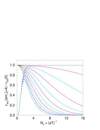
Figure 1: Discretized energy density of free fermions with $am=0,0.1,\cdots,1$.

As this is a free field calculation, the scale is set explicitly by specifying the dimensionful temperature $T$. The infrared cutoff given by the spatial extent of the lattice can be specified in terms of the dimensionless aspect ratio: $\zeta\equiv VT^{3}$. The ultraviolet cutoff given by the lattice spacing can by specified in terms of the dimensionless $N_{4}\equiv(aT)^{-1}$. If we choose $a,V$ so that the product $\zeta N_{4}$ is an integer, then the discretized analogue of (1) is

$$\frac{\varepsilon_{\rm disc}(m)}{T^{4}}=\frac{4}{\zeta^{3}}\sum_{p}\frac{aN_{4}\sqrt{p^{2}+m^{2}}}{1+\exp(aN_{4}\sqrt{p^{2}+m^{2}})}$$ (2)

where the sum is over $-\pi/a\leq p<\pi/a$ with spacing $\Delta p=2\pi/\zeta N_{4}a$.

In figure 1, we display the both the SB (1) and discretized (2) energy densities at fixed aspect ratio $\zeta=4$ for various $N_{4}$ and masses from $am=0$ to 1 spaced in 0.1 intervals. For high temperatures (small $N_{4}$), the mass of the fermions becomes irrelevant and the SB (solid) lines converge on $\varepsilon_{\rm SB}(0)$. In this same limit, the number of allowed lattice momenta becomes small so the discretized (dashed) lines are cutoff and converge on zero. For this aspect ratio, the SB and discretized values differ by more than a percent for $N_{4}\leq 4$.

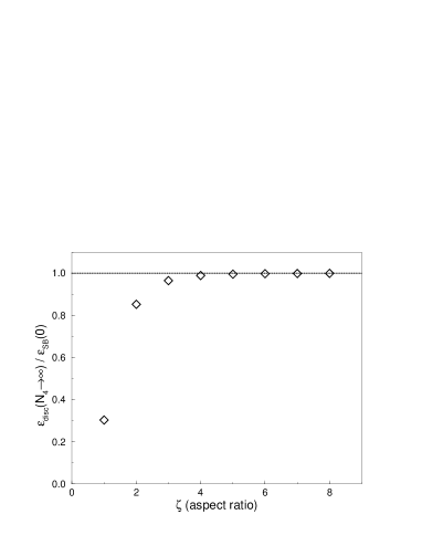
Figure 2: Discretized massless energy density vs. aspect ratio.

In figure 1, the massless discretized energy density falls short of the SB limit, approaching 0.989 as $N_{4}\to\infty$. For massless fermions, even small momenta contribute at all temperatures, and these are cutoff by the aspect ratio $\zeta=4$. In figure 2, we show the massless discretized energy density vs. aspect ratio in the $N_{4}\to\infty$ limit. So, from just the continuum free dispersion relation and a simple discretization procedure, lattice simulations should not expect to reproduce the continuum energy density to better than a few percent on any lattice smaller than $16^{3}\times 4$.

3 Comparing free Wilson fermions

The energy density of free Wilson fermions has been known for a long time [2] and its large overestimation of the SB limit at smaller values of $N_{4}$ has often been used as an argument against the applicability of Wilson thermodynamics at currently accessible lattice spacings. Because standard domain wall and overlap fermions use Wilson terms to give mass to the doubler species, we might anticipate that similar effects may be seen in the energy density of these fermion formulations. So, we would like to first understand free Wilson thermodynamics.

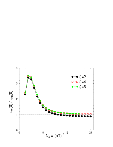
Figure 3: Energy density of free Wilson fermions.

We show the energy density of free massless Wilson fermions vs. $N_{4}$ for three aspect ratios in figure 3. As in the discretized case of section 2, approaching the $N_{4}\to\infty$ limit at fixed small aspect ratio underestimates the SB result. However, the most obvious feature is the large overestimation of the SB result at smaller $N_{4}$. At the smallest $N_{4}$, at least, we now can understand that the energy density is cutoff by the scarcity of lattice momenta.

Figure 4: Discretized energy density with fifteen “doublers.”

We propose a simple model to reveal the source of the overestimate for Wilson fermions. Without the Wilson term, the energy density of free naive lattice fermions would be 16 times larger than the SB result. The Wilson term gives 15 doublers a mass proportional to the cutoff. But from figure 1, we expect these now massless doublers to make a significant contribution to the overall Wilson energy density until $N_{4}\gtrsim 8$. To emphasize the point, in figure 4 we compare the free Wilson energy density with that of one massless and fifteen massive flavors using the discretized energy density (2). While more effort could be made to adjust the masses of the discretized doublers to make the two curves agree, from the common shape we believe this is a good explanation of the Wilson excess.

4 Anisotropic domain wall action

The energy density is formally given by

$$-\varepsilon\equiv\frac{1}{V}\left.\frac{\partial\ln Z}{\partial T^{-1}}\right|_{V}.$$ (3)

In order to vary the temperature continuously while holding the volume fixed to compute the derivative, we must allow the lattice spacing in the temporal direction, $a_{4}$, to differ from the spatial direction, $a$. The ratio of the spacings is the anisotropy $\xi\equiv a/a_{4}$. Of course, once the derivative has been computed we can take the isotropic limit, $\xi\to 1$.

To derive the form of the anisotropic domain wall and overlap fermion matrix, we choose the interpretation of the extra dimension in the domain wall formalism as a flavor space. We start from Klassen’s anisotropic Wilson action [4] without the anisotropic clover terms as the domain wall action is ${\cal O}(a)$ improved in the $L_{s}\to\infty$ limit. Using the conventions of the Columbia group [5] the anisotropic domain wall action is

$$D_{F}(x,s;x^{\prime},s^{\prime})=\delta_{s,s^{\prime}}D^{\parallel}(x,x^{\prime})+D^{\perp}(s,s^{\prime})\delta_{x,x^{\prime}}$$ (4)

$$D^{\parallel}(x,x^{\prime})=\sum_{\mu=1}^{4}\xi^{z_{\mu}}\frac{\nu_{\mu}}{2}\left[\left(1-\gamma_{\mu}\right)U_{\mu}(x)\delta_{x+\hat{\mu},x^{\prime}}\right.$$

$$+\left.\left(1+\gamma_{\mu}\right)U_{\mu}^{\dagger}(x^{\prime})\delta_{x-\hat{\mu},x^{\prime}}\right]$$

$$+\left[m_{0}-r\left(3\xi^{z}\nu+\xi^{z_{4}}\nu_{4}\right)\right]\quad$$ (5)

where the $\nu_{\mu}$ are the bare velocities of light with $\nu_{1}=\nu_{2}=\nu_{3}\equiv\nu$, the anisotropy is $\xi\equiv a/a_{4}$, and the exponents $z_{\mu}$ are set to $z_{1}=z_{2}=z_{3}\equiv z=0$ and $z_{4}=1$ although other choices are possible if they satisfy the constraint $z_{4}-z=1$ [6]. The flavor mixing matrix $D^{\perp}(s,s^{\prime})$ is the same as written by the Columbia group [5] without any extra coefficients since the normalization of the fermion fields was shifted so that no coefficients appear with the $m_{0}$ term in the action. The domain wall action includes a Pauli-Villars subtraction at $m_{f}=1$ to cancel the bulk infinity from the $L_{s}$ heavy flavors at the mass scale $m_{0}$.

Following Neuberger [7], the anisotropic form of the overlap action can be derived as the $L_{s}\to\infty$ limit of the anisotropic domain wall action. However, the form of the action is easy to guess: just replace the isotropic Wilson matrix with the anisotropic one in the overlap Hamiltonian.

5 Domain wall/overlap energy density

From (3), the energy density is computed explicitly using

$$\frac{\varepsilon_{F}}{T^{4}}=\left(\frac{1}{\xi\zeta}\right)^{3}{\rm Tr~{}}\left[D_{F}^{-1}\xi\frac{\partial}{\partial\xi}D_{F}\right].$$ (6)

Our approach was to compute the derivative $\xi\partial/\partial\xi D_{F}$ analytically and then diagonalize (6) into blocks indexed by four-momentum $p_{\mu}$ using Fourier transform. Each block matrix $\widetilde{D}_{F}(p)$ was inverted numerically and then the traces were summed over all four-momenta. In general, (6) is computed twice, once on a $(\zeta N_{4})^{3}\times N_{4}$ lattice and again on a $(\zeta N_{4})^{4}$ lattice for the $T=0$ vacuum subtraction. Anti-periodic boundary conditions were imposed in the temporal direction in both cases. For domain wall fermions, the calculation is repeated with the Pauli-Villars mass and the difference is used, schematically $\varepsilon_{\rm dwf}=[\varepsilon_{F}(T)-\varepsilon_{F}(0)]-[\varepsilon_{PV}(T)-\varepsilon_{PV}(0)].$

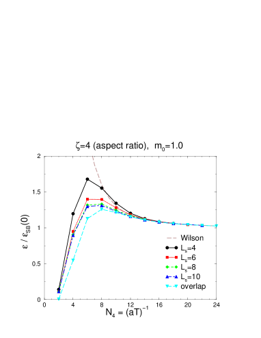
Figure 5: Domain wall and overlap energy density at $m_{0}=1$.

The energy density for domain wall fermions at various $L_{s}$ and overlap fermions are shown in figure 5. The choice $m_{0}=1$ is the optimal free field value in the sense that the surface mode with $p_{\mu}=0$ is completely localized to the domain wall. However, surface modes with other momenta will have finite exponential decay rates so the $L_{s}$ dependence is due to these modes. The energy density at $L_{s}=10$ is nearly converged on the $L_{s}\to\infty$ limit. Any small differences between the domain wall and overlap at smaller $N_{4}$ may be due to the different treatment of the spacing of sites in the extra dimension. This is currently under study.

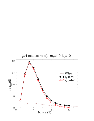
Figure 6: Domain wall fermion and Pauli-Villars energy densities.

The Wilson energy density is also shown in figure 5. Based on arguments of section 3, the reduced excess energy density for domain wall and overlap fermions indicates the participation of the heavy doublers in the thermodynamics is suppressed due to Pauli-Villars term. In figure 6 we show the energy density of domain wall fermions before Pauli-Villars subtraction and separately the energy density of the Pauli-Villars regulators. Before subtraction, the excess energy density due to heavy modes is essentially $L_{s}$ times larger than the Wilson case, again shown as a dashed line. That the domain wall density of order one appear as the difference of two densities of order $L_{s}$ suggests tinkering with the Pauli-Villars subtraction may reduce heavy contributions further. However, it is unclear how worthwhile a lengthy study of possible Pauli-Villars terms would be when the benefits of such a finely tuned action may vanish in the interacting case.

6 “Doubly” regularized fermions

As pointed out by Neuberger [7], lattice fermion actions with Pauli-Villars subtractions are “doubly” regularized, once by the lattice spacing and again by the Pauli-Villars pseudofermions. In section 5, we claim the Pauli-Villars suppression of heavy contributions to the domain wall energy density works so well the end result is an improvement over Wilson fermions quite apart from any issues of chiral symmetry. However, there is no reason we can’t attempt to use a Pauli-Villars regulator to achieve the same result for Wilson fermions.

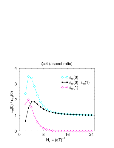
Figure 7: Energy density of “doubly” regularized Wilson fermions.

In figure 7 we show the Wilson energy density before Pauli-Villars subtraction, as has already appeared in the last several figures as open circles, the energy density of the proposed Pauli-Villars regulators with a mass of $m_{0}=1$ as open diamonds and the doubly regularized Wilson energy density appears as filled squares. After the subtraction, the contribution of heavy modes to energy density is substantially reduced. Fine tuning of the Pauli-Villars mass to make the energy density agree with the Stefan-Boltzmann limit at a given $N_{4}$ is certainly possible, but it is again unclear how to do this in the interacting case.

Another potential advantage of doubly regularized fermion formulations is that the quenched theory is recovered when the fermion mass is set to the Pauli-Villars mass. An example of its usefulness is a proposed calculation of the dynamical QCD equation of state in the deconfined phase using the integral method. As the integration contour originates in the strong coupling regime and crosses through the transition region, an inordinate amount of work must be done before anything is known of the deconfined region. As the quenched theory appears as a different contour of fixed finite mass, one could use the integration contour shown in figure 8. As the quenched equation of state is already well known for several $N_{4}$ [3], all dynamical simulations are performed only at weaker couplings where fermion algorithms are usually better conditioned.

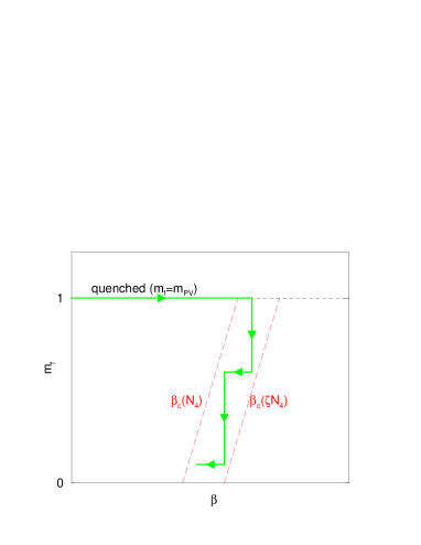
Figure 8: Integration contour for deconfined equation of state

One subtlety of integrating ”off the quenched contour” is the importance of computing the $T=0$ vacuum subtraction at as low a temperature as possible. As before, finite temperature observables are computed on $(\zeta N_{4})^{3}\times N_{4}$ lattices and $T=0$ subtractions are computed on $(\zeta N_{4})^{4}$ lattices. On the quenched contour $(aT)^{-1}=\zeta N_{4}$ lattices may be confined, but while integrating down at fixed coupling, one may enter the $\zeta N_{4}$ transition region. To avoid this, a stair step contour could be used.

We would like to thank N. Christ, R. Mawhinney, T. Klassen and P. Vranas for useful discussions in the early stages of this work.

References

- [1]
- [2] J. Engels et al., Nucl. Phys. B205, 239 (1982).
- [3] F. Karsch, Nucl. Phys. Proc. Suppl. 83, 14 (2000). [hep-lat/9909006].
- [4] T. R. Klassen, Nucl. Phys. Proc. Suppl. 73, 918 (1999) [hep-lat/9809174].
- [5] P. Chen et al., hep-lat/0006010.
- [6] R. C. Trinchero, Nucl. Phys. B227, 61 (1983).
- [7] H. Neuberger, Phys. Rev. D57, 5417 (1998) [hep-lat/9710089].