LATTICE SUPERSYMMETRY WITH DOMAIN WALL FERMIONS

Supersymmetry, like Poincaré symmetry, is softly broken at finite lattice spacing provided the gaugino mass term is strongly suppressed. Domain wall fermions provide the mechanism for suppressing this term by approximately imposing chiral symmetry on the lattice. We present the first numerical simulations of ${\cal N}=1$ supersymmetric ${\rm SU}(2)$ Yang-Mills on the lattice in $d=4$ dimensions using domain wall fermions.

1 Introduction

Supersymmetric (SUSY) field theories may play an important role in describing the physics beyond the Standard Model. Non-perturbative numerical studies of these theories could provide confirmation of existing analytical calculations and new insights on aspects of the theories not currently accessible to analytic methods, similar in spirit to the current situation in many other field theories, most notably QCD. Several, but not all, SUSY theories can be formulated and studied numerically on the lattice $\!{}^{{\bf?},{\bf?},{\bf?}}$. Foremost, as the lattice spacetime is discreet, only a discrete subgroup of the Poincaré symmetry is unbroken, so any formulation will break SUSY. However, the allowed operators that break Poincaré symmetry are irrelevant in the continuum limit, so one can calculate at several lattice spacings $a$ and take the $a\to 0$ limit.

If a SUSY model has non-trivial scalar fields, scalar mass terms will break SUSY unless forbidden by some symmetry. Since these operators are relevant fine tuning will be needed to cancel their contributions in the continuum limit. We avoid this problem as the four-dimensional ${\cal N}=1$ Super Yang-Mills (SYM) theory does not involve scalars. The lattice fermion doubling problem will also break SUSY due to a mismatch in the number of bosonic and fermionic degrees of freedom. Removing doublers breaks chiral symmetry, allowing relevant gluino mass terms. In the traditional approach $\!{}^{{\bf?}}$, fine tuning is used to cancel these mass terms. Pioneering work using these methods has already produced very interesting numerical results $\!{}^{{\bf?},{\bf?}}$.

Many properties of the ${\cal N}=1$ SYM have already been computed using analytic techniques that take particular advantage of the supersymmetry in the model. On the contrary, numerical simulations of SYM are at least as computationally difficult as dynamical QCD. So, one must be careful to choose an interesting problem since the trade-off is to not study some aspect of dynamical QCD. For us, one such interesting problem is to determine if the vacuum supports a non-zero gluino condensate $\left\langle\overline{\chi}\chi\right\rangle$, as widely believed, and whether the formation of the condensate is due to spontaneous or anomalous symmetry breaking.

The Dirac operator in the adjoint representation of ${\rm SU}(N)$ has an index $2N\nu$, where $\nu$ is the winding of the gauge field. Classical instantons have integer winding and cause condensations of operators with $2N$ gluinos which anomalously breaks the ${\rm U}(1)$ $R$-symmetry to ${\rm Z}_{2N}$. For $\left\langle\overline{\chi}\chi\right\rangle$ to condense, the remaining ${\rm Z}_{2N}$ symmetry must further break either spontaneously or anomalously to $Z_{2}$. If the breaking is anomalous, then the responsible gauge configurations must have fractional winding $\!{}^{{\bf?}}$. It has already been established that such gauge configurations do exist $\!{}^{{\bf?}}$. It is our goal to distinguish between these two scenarios.

This work summarizes results recently presented by the author in collaboration with John B. Kogut and Pavlos M. Vranas $\!{}^{{\bf?}}$. All numerical simulations were run on QCDSP supercomputers at Columbia Univ. and Ohio State. For reviews on DWF please see the LATTICE ’00 review talk of Vranas $\!{}^{{\bf?}}$ and references therein. The possible use of DWF in SUSY theories has been discussed in earlier works $\!{}^{{\bf?},{\bf?}}$ and the methods used here are along these lines. For lists of references not included here for lack of space, please see the cited articles $\!{}^{{\bf?}}$.

2 The DWF formulation

In the lattice DWF formulation of a vector-like theory in $d=4$ dimensions, the fermionic fields are defined on a $d+1$ dimensional lattice using a local action. It is often convenient to treat the extra dimension as a new internal flavor space. Thus, the gauge fields are introduced in the standard way in the $d$ dimensional spacetime and are coupled to the extra fermion degrees of freedom like extra flavors. The detailed form of the action can be found in our recent work $\!{}^{{\bf?}}$.

The key ingredient is the free boundary conditions imposed on the extra dimension. As a result, two chiral exponentially bound surface states appear on the boundaries (domain walls) with the plus chirality localized on one wall and the minus chirality on the other. The two chiralities mix only by an amount that is exponentially small in the size of the extra dimension, called $L_{s}$, and together form a Dirac spinor that propagates in the $d$ dimensional spacetime with an exponentially small mass. Therefore, the chiral symmetry breaking artificially induced by the Wilson term can be controlled by the new parameter $L_{s}$. It is often convenient to introduce an additional bare gluino mass $m_{f}$ to help control extrapolations to the chiral limit. In the $L_{s}\to\infty,m_{f}\to 0$ limit chiral symmetry is exact at any lattice spacing without fine tuning.

The computing requirement is linear in $L_{s}$, in contrast to traditional lattice fermion regulators where the chiral limit is approached only as the continuum limit is taken, a process that is achieved at a large computing cost. Specifically, because of algorithmic reasons, the computing cost to reduce the lattice spacing by a factor of two grows by a factor of $2^{8-10}$ in four dimensions. Therefore, the unique properties of DWF provide a way to bring under control the systematic chiral symmetry breaking effects using today’s supercomputers.

The application of DWF to ${\cal N}=1\ {\rm SU}(N)$ SYM is quite similar to $N_{f}=1\ {\rm SU}(N)$ QCD. The differences are merely that the fermions are in the adjoint representation of ${\rm SU}(N)$ and that the Dirac fermion fields must satisfy the Majorana constraint, thereby reducing by half the number of fermion degrees of freedom. After integrating out the Grassmann fields subject to the Majorana constraint, the Dirac determinant is replaced by a Pfaffian: essentially the square root of the determinant, provided it is positive. For DWF, the Pfaffian cannot change sign so working with either Pfaffians or square roots of determinants is equivalent.

3 Numerical results

All numerical simulations were performed on $8^{4}$ and $4^{4}$ spacetime volumes using the inexact hybrid molecular dynamics (HMD) $R$ algorithm. The algorithm numerically integrates the classical equations of motion as part of generating a statistical ensemble with weights proportional to the fourth root of a two adjoint flavor Dirac determinant. For DWF, this weight is proportional to a single adjoint Majorana flavor. The step sizes were chosen such that systematic uncertainties due to numerical integration errors are negligible compared to statistical uncertainties.

Figure 1: Wilson line $\left\langle\left|W\right|\right\rangle$ on an $8^{4}$ lattice. Diamonds are quenched and the cross is dynamical with $L_{s}=24$ and $m_{f}=0$.

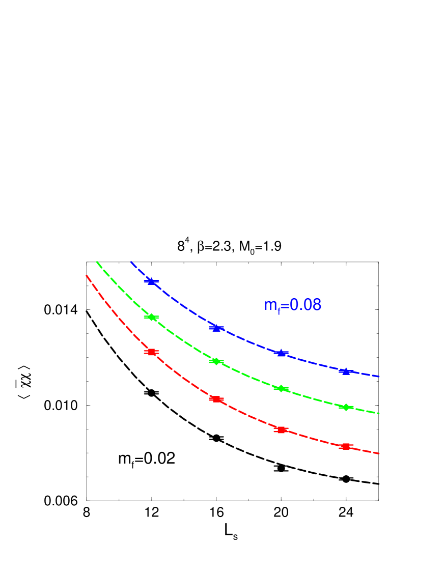
Figure 2: Gluino condensate $\left\langle\overline{\chi}\chi\right\rangle$ vs. $L_{s}$ with $\beta=2.3$ and $m_{f}=0.02,0.04,0.06,0.08$. Curves are an exponential fit.

The $8^{4}$ volume simulations were done with $\beta\equiv 4/g^{2}=2.3$. The value of $\beta$ was chosen as large as possible without entering the thermal transition region. From quenched simulations in an $8^{4}$ volume, the magnitude of the fundamental Wilson line $\left\langle\left|W\right|\right\rangle$, the quenched order parameter, is plotted vs. $\beta$ in figure 2. The value of $\left\langle\left|W\right|\right\rangle$ from a simulation of the dynamical theory at $\beta=2.3$ is also shown (cross), indicating that the dynamical theory is in a phase that “confines” fundamental sources. Therefore, the box size is large enough to avoid thermal effects that break SUSY. Using similar arguments, the $4^{4}$ volume simulations were done with $\beta=2.1$, near the limit of the weak coupling regime. Scaling arguments appropriate for weak coupling suggest that the lattice spacing at $\beta=2.1$ is twice as large as at $\beta=2.3$.

To extrapolate the measured values of $\left\langle\overline{\chi}\chi\right\rangle$ to the chiral limit, $L_{s}\to\infty$ and $m_{f}\to 0$, simulations were performed in $8^{4}$ volumes at fixed $\beta=2.3$ while the size of the extra dimension $L_{s}$ was varied between 12 and 24 and the bare mass $m_{f}$ was varied between 0.02 and 0.08. The measured values appear as the points in figure 2. According to Leutwyler and Smilga $\!{}^{{\bf?}}$, if the formation of the gluino condensate is due to spontaneous symmetry breaking, the lattice volume limits how small the dynamical qluino mass can be set without losing the condensate: $12m_{\rm eff}\left\langle\overline{\chi}\chi\right\rangle V\gg 1$ (the 12 is just normalization). As $m_{\rm eff}\gtrsim m_{f}$, this limit is satisfied for all $8^{4}$ simulations with $m_{f}\geq 0.02$.

To estimate the gluino condensate in the chiral limit, we first extrapolate at fixed $m_{f}$ to the $L_{s}\to\infty$ limit using the fit function $\left\langle\overline{\chi}\chi\right\rangle=c_{0}+c_{1}\exp(-c_{2}L_{s})$. The best fit functions are plotted as the curves in figure 2. The values of the extrapolated gluino condensate (with propagated errors) appear as points in figure 4. These extrapolated values are then further extraploted to the $m_{f}\to 0$ limit using a linear function $\left\langle\overline{\chi}\chi\right\rangle\left(L_{s}\to\infty\right)=b_{0}+b_{1}m_{f}$. The best fit function appears as the line in figure 4. It is also reassuring to note that reversing the order of limits, i. e.  first $m_{f}\to 0$ at fixed $L_{s}$ then $L_{s}\to\infty$, yields a statistically consistent answer.

Figure 3: Extrapolated $\left\langle\overline{\chi}\chi\right\rangle$ to $L_{s}\to\infty$ limit vs. $m_{f}$ and linear fit to $m_{f}\to 0$ limit.

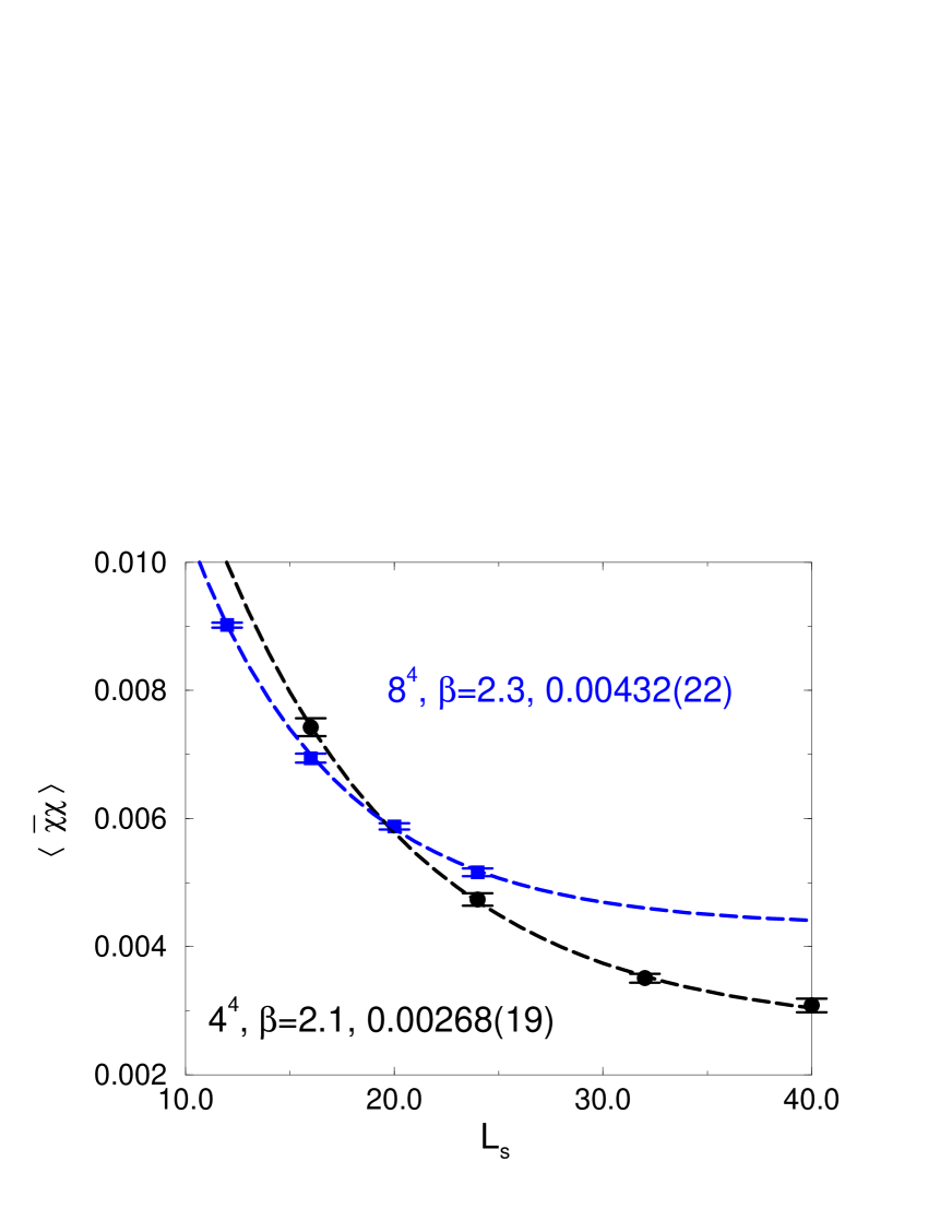
Figure 4: Dynamical $\left\langle\overline{\chi}\chi\right\rangle$ at $m_{f}=0$ vs. $L_{s}$ on an $8^{4}$ lattice at $\beta=2.3$ and a $4^{4}$ lattice with $\beta=2.1$. Curves are exponential fits.

Another approach to estimating the gluino condensate in the chiral limit is to actually perform dynamical simulations with $m_{f}=0$. Since finite $L_{s}$ will induce an exponentially small breaking of chiral symmetry, the effective gluino mass will not be zero. However, the gluino mass should be too small to support spontaneous symmetry breaking. Additional simulations were run for $L_{s}=12,16,20,24$. The data are shown in figure 4. The curve is the best fit to the exponential fitting function with the extrapolated value of the condensate as shown.

Surprisingly, both methods for estimating the gluino condensate produce consistent results within the statistical errors. Note that this is inconsistent with the notion of spontaneous symmetry breaking. Operationally, this result reinforces our claim that systematic uncertainties are still relatively small despite limited statistical precision. Further, it gives us some confidence that our fit functions are valid over the region of interest.

To further check for spontaneous symmetry breaking of the ${\rm Z}_{4}$ symmetry, we measured $\left\langle\overline{\chi}\chi\right\rangle$ on smaller $4^{4}$ lattices with $m_{f}=0$ and even larger values for $L_{s}$. The data are shown in figure 4 with the best exponential fit and the extrapolated value for the condensate. This provides even stronger evidence that spontaneous symmetry breaking is not responsible for the formation of a gluino condensate, at least in finite volumes. On these lattices $12m_{f}V\left\langle\overline{\chi}\chi\right\rangle<1$, so analytical considerations $\!{}^{{\bf?}}$ suggest the support of $\left\langle\overline{\chi}\chi\right\rangle$ must come primarily from topological sectors with fractional winding of $\nu=\pm 1/2$.

The spectrum of the theory is of great interest but it was not possible to measure it on the small lattices considered here. Also, the gluino condensate was measured at only two different lattice spacings so extrapolation to the continuum limit to compare with analytical results is not possible. Future work could explore these very interesting topics.

References

- [1]
- [2] G. Curci and G. Veneziano, Nucl. Phys. B292, 555 (1987).
- [3] H. Neuberger, Phys. Rev. D57, 5417 (1998) [hep-lat/9710089].
- [4] D. B. Kaplan and M. Schmaltz, Chin. J. Phys. 38, 543 (2000) [/hep-lat/0002030].
- [5] I. Campos et al. [DESY-Münster Collaboration], Eur. Phys. J. C11, 507 (1999) [hep-lat/9903014].
- [6] A. Donini, M. Guagnelli, P. Hernandez and A. Vladikas, Nucl. Phys. B523, 529 (1998) [hep-lat/9710065].
- [7] G. T. Fleming, J. B. Kogut and P. M. Vranas, hep-lat/0008009.
- [8] R. G. Edwards, U. M. Heller and R. Narayanan, Phys. Lett. B438, 96 (1998) [hep-lat/9806011].
- [9] P. M. Vranas, hep-lat/0011066.
- [10] H. Leutwyler and A. Smilga, Phys. Rev. D46, 5607 (1992).