UPRF-2000-16

SWAT: 281

November 2000

A consistency check for Renormalons in Lattice Gauge Theory: $\beta^{-10}$ contributions to the $SU(3)$ plaquette

F. Di Renzo$\,{}^{a}$, and L. Scorzato$\,{}^{a,b}$

${}^{a}\,$Dipartimento di Fisica, Università di Parma
and INFN, Gruppo Collegato di Parma, Italy ${}^{b}\,$Department of Physics,
University of Wales at Swansea, United Kingdom

Abstract

We compute the perturbative expansion of the Lattice $SU(3)$ plaquette to $\beta^{-10}$ order. The result is found to be consistent both with the expected renormalon behaviour and with finite size effects on top of that.

1 Introduction

In recent years, the Numeric implementation of Stochastic Perturbation Theory (NSPT) was introduced, which was able to reach unprecedented high orders in pertubative expansions in Lattice Gauge Theory (LGT). The historic success of NSPT was the computation of the Lattice $SU(3)$ basic plaquette to order $\beta^{-8}$[1]. This led to the possibility of actually verifying the expected dominance of the leading InfraRed (IR) Renormalon [2] associated to a dimension four condensate. The computation was performed on a $8^{4}$ lattice. We are now in a position to quote results to a reasonable accuracy for the perturbative expansion of the same quantity to order $\beta^{-10}$ on both a $8^{4}$ and a $24^{4}$ lattice.
There are at least three main motivations for such a computation. First of all, it provides a clear consistency argument in support of the conclusions of our previous work. The results in [1] are actually the only ones from which one can recognize the presence of renormalons by direct inspection of the perturbative coefficients of a QCD quantity. Ironically, this is true in a scheme (the lattice) which one would never choose for a high order QCD calculation in a standard (as opposed to NSPT) approach. We will give strong evidences that a very good control has been taken over both the IR renormalon growth and the finite size effects on top of that. In particular, finite size effects have always been a matter of concern for the computation. They play a fundamental role since they impinge on the IR region which is responsible for the renormalon growth. Basically, the higher is the loop, the lower are the (IR) momenta which give the main contribution. In view of this one could be worried that one is missing important contributions on the $8^{4}$ lattice on which the NSPT perturbative computations were first performed on. In [3] evidences from the non linear sigma models were collected which suggested that renormalon growth was not substantially tamed at the eight loop level. We can now strengthen our confidence that the leading behaviour had been actually properly singled out in our previous work. On top of that we are now in a position to assess the finite size effects, which turn out to be of the order of a few percent at the order we got.
While the eight loop expansion in [1] was a major success, it actually opened more problems than it settled down and this sets the stage for the second motivation for our present computation. There was a longstanding problem concerning the possibility of determining the Gluon Condensate (GC) from LGT by a method which actually relied on the computation of high orders in the perturbative expansion of the plaquette. The latter is the lattice representation for the GC and its perturbative expansion is an additive renormalisation which is by far the leading contribution at the value of $\beta$ usually taken into account. This perturbative contribution can be seen as the contribution coming from the identity operator in the Operator Product Expansion (OPE) for the plaquette. The key point is that in this OPE there is no space for an order $a^{2}$ term, a gauge invariant operator of dimension two missing. Next term in OPE is expected to be an $a^{4}$ contribution associated with the genuine GC. The old approach to the problem was to subtract the first (perturbative) contribution from Monte Carlo measurements of the plaquette in order to single out the $a^{4}$ term (the GC) [4]. The signature of such a term can be recognized by performing the subtraction at different values of $\beta$ and looking for the scaling dictated by Asymptotic Freedom. The actual problem is that the series for the plaquette “not only has to be subtracted, it has to be defined in first place”. Due to the presence of the IR renormalon, the series has an ambiguity in different prescriptions for resumming it which is just the same order as the GC, i.e. an $a^{4}$ contribution. Being aware of this, the most striking point is that by performing the subtraction, with any given prescription, one is left with an $a^{2}$ contribution, at least on the $8^{4}$ lattice the computation was first performed on [5]. The problem challenges our understanding of potentially any short-distance expansion and so it needs to be cleared up. At the moment more than one explanation appear to be possible. The effect could either be a pure lattice artifact or a fundamental issue. With respect to the latter hypothesis, [5] suggested the effect of UltraViolet (UV) contributions to the running coupling. Since the time of [5] the phenomenology of non–standard $Q^{-2}$ power effects has actually been reported growing. In particular, the work in [6] establishes a relation between a dual superconductor confinement mechanism and “OPE–violating” corrections. In this paper we do not want to enter at all the $a^{2}$–affair. Still, the reliability of our previous perturbative computations has to be assessed with this question in mind. Given the potential impact of the result in [5], we want to be sure that nothing was wrong with respect to the Renormalon contribution extraction, leaving for a subsequent publication [7] a refinement of the whole analysis concerning the subtraction procedure. We stress that such a refinement will in particular benefit by the study of finite size effects.
Finally something can be learned from the computation about the NSPT method itself. The present result establishes the highest order ever reached by NSPT in LGT. In [8] a word of caution was spent on uncritical application of the method, stressing the issue of a careful assessment of statistical errors. Ironically enough, it was pointed out that problems plague simple models much more than complex systems like Lattice $SU(3)$. We refer the reader to a future publication [9] for a more organic report on the application of the NSPT method to LGT. Still, it is reassuring (although of course admittedly not a proof of reliability of the method) to note that in the context of this work there is a fine agreement between the results obtained by our stochastic method and those inferred by a (maybe strong) theoretical prejudice.
The paper is organized as follows. In Sect. 2 we recall the basics of IR Renormalon analysis applied to a $dim=4$ condensate and write the formulas relevant for a finite lattice, which are the foundations of our subsequent analysis. In Sect. 3 we present our results for the first ten coefficients in the expansion of the plaquette both on a $8^{4}$ and on a $24^{4}$ lattice, showing that they are consistent with the Renormalon factorial growth and with the expected finite size effects on top of that. Sect. 4 contains our conclusions and perspectives for future work. An appendix covers algebraic details.

2 The IR Renormalon on a finite lattice

We start by writing first of all the definition of our observable, that is the basic plaquette normalised as

$$W(M)\,=\,1-\mbox{\small${{1}\over{3}}$}\left\langle\mbox{Tr}\;U_{p}\right\rangle\,,$$ (1)

$U_{p}$ being the product of links around a $1\times 1$ Wilson Loop. We write an explicit dependence on the size ($M$) of the lattice on which the osbervable is computed. In Perturbation Theory

$$W(M)=\sum_{\ell=1}c^{(M)}_{\ell}\beta^{-\ell}$$ (2)

Next we move to recall the main points of Renormalon analysis. Notations are slightly different from those of [1, 5] and closer to those of [3]. The aim of this section is anyway to be self–contained.

2.1 Basics on the factorial growth of perturbative coefficients

The expected form for a dimension $4$, Renormalisation Group invariant condensate is written as

$$W=\int^{Q^{2}}_{0}\;{{k^{2}\,dk^{2}}\over{Q^{4}}}\;f(k^{2}/\Lambda^{2})\,.$$ (3)

$Q$ is in our case the UV cutoff fixed by the lattice spacing: $Q=\pi/a$. Given the above dimensional and R.G. arguments, $f(k^{2}/\Lambda^{2})$ is a dimensionless function independent on the scale $Q$, for large $Q$, and can thus be expressed in terms of a running coupling at the scale $k^{2}$. One obtains the Renormalon contribution by considering the high frequencies contribution to Eq. (3), that is

$$W^{\rm ren}=C\;\int^{Q^{2}}_{r\Lambda^{2}}\;{{k^{2}\,dk^{2}}\over{Q^{4}}}\;\alpha_{\sf s}(k^{2})\,,$$ (4)

in which $f(k^{2}/\Lambda^{2})$ has been taken proportional to the perturbative running coupling (higher powers of the coupling simply result in subleading corrections to the formulas we will get this way). We now introduce the variable

$$z\equiv z_{0}\left(1-{\alpha_{\sf s}(Q^{2})}/{\alpha_{\sf s}(k^{2})}\right)\,,\;\;\;\;\;\;\;z_{0}\equiv{{1}\over{3b_{0}}}\,,$$ (5)

using which together with the two loop form for $\alpha_{\sf s}(k^{2})$ results in

$$W^{\rm ren}={\cal N}\int_{0}^{z_{0_{-}}}dz\;e^{-\beta z}\;(z_{0}-z)^{-1-\gamma}\,.$$ (6)

In the last equation we have traded $\alpha_{\sf s}(k^{2})$ for the $\beta$ coupling one is more familiar with on the lattice and introduced a couple of new symbols according to

$$4\pi\alpha_{\sf s}(Q^{2})\equiv{6}/{\beta}\,,\;\;\;\;\;\;\;\gamma\equiv 2{{b_{1}}\over{b_{0}^{2}}}\,,\;\;\;\;\;\;\;0<z<z_{0_{-}}\equiv z_{0}(1-\alpha_{\sf s}(Q^{2})/\alpha_{\sf s}(r\Lambda^{2}))\,.$$ (7)

In the equations above $b_{0}$ and $b_{1}$ are the first and second coefficients of the perturbative $\beta$–function (to fix normalisation: $b_{0}=11/(4\pi)^{4}$). $z_{0_{-}}$ is clearly reminiscent of the IR cutoff $r\Lambda^{2}$ imposed in Eq. (4) to avoid Landau pole once the perturbative coupling had to be plugged in. From Eq. (6) it is now easy to obtain a perturbative expansion

$$W^{\rm ren}=\sum_{\ell=1}\;\beta^{-\ell}\;\{c^{ren}_{\ell}+{\cal O}(e^{-z_{0}\beta})\}\,,\;\;\;\;\;\;\;c^{ren}_{\ell}={\cal N^{\prime}}\;\Gamma(\ell+\gamma)\;z_{0}^{-\ell}\,.$$ (8)

The factorial growth of the series is the Renormalon contribution, while the ${\cal O}(e^{-z_{0}\beta})$ is again coming from the IR cutoff $r\Lambda^{2}$ in Eq. (4). Naively one could have not imposed any IR cutoff before going from the ill-defined (because of the Landau pole) integral to the series. The factorial growth would have anyway asked for the ${\cal O}(e^{-z_{0}\beta})$ contribution in order to obtain a resummation of the series. Actually the reader familiar with the subject has most probably well recognized in Eq. (6) a Borel representation.

2.2 The factorial growth on a finite lattice

Apart from the explicit reference to the lattice spacing in the UV cutoff we have till now adhered to a continuum notation, implicitly assuming some continuum scheme in which for example Eq. (3) is defined. We now move to rewrite such a representation on a finite lattice. One can consider (notice that we now explicitly write the dependence on the number of lattice points $M$)

$$W^{\rm ren}(M)=C\;\int^{Q^{2}}_{Q_{0}^{2}(M)}\;{{k^{2}\,dk^{2}}\over{Q^{4}}}\;\alpha_{\sf s}(sk^{2})\,.$$ (9)

The lower limit of integration is the explicit IR cutoff imposed by the finite extent of the lattice ($Q_{0}(M)=2\pi/Ma$), while the scale $s$ is in charge of matching from a continuum to a lattice scheme. In view of that and since rescaling $k^{2}\rightarrow sk^{2}$ amounts to rescaling $\Lambda\rightarrow s^{-1/2}\Lambda$, it is likely to expect for $s$ a value $s=K^{-2}$ consistent (up to an eventual further change of scale) with $\Lambda_{cont}=K\Lambda_{latt}$ for some continuum scheme. By a change of variable in the integral it is easy to trade the rescaling of the argument of $\alpha_{\sf s}$ for a rescale of $Q^{2}\rightarrow sQ^{2}$ (and similarly for the lower limit of integration). Remember that in the previous section we obtained an expansion in the coupling defined at the scale $Q$: at one loop level a change of scale in the coupling is equivalent to a change of scheme, and this matches the present notation to the notation of [1, 5]. Given Eq. (9), one can of course perform the same change of variable defined in Eq. (5) and obtain a new power expansion. In order not to have the main message of the procedure obscured by trivial algebra, we collect the details in an appendix. One is left with

$$W^{\rm ren}(M)=\sum_{\ell=1}\;\beta^{-\ell}\,c^{ren}_{\ell}(M;s,C)$$ (10)

The coefficients $c^{ren}_{\ell}(M;s,C)$ can be expressed in terms of incomplete $\Gamma$ functions (see the appendix). It is important to notice their dependences. They depend trivially (i.e. multiplicatively) on the overall constant $C$ which is present in Eq. (9) to account for everything which is subleading. They also depend on the scale $s$ which is in charge of the matching to the scheme in which Eq. (4) best describes the expansion (remember that one does not know that a priori). Finally, they depend parametrically on the lattice size $M$. The attitude to take with respect to Eq. (10) is now the same as in [1, 5], that is: can one determine values $C=\bar{C}$ and $s=\bar{s}$ by fitting the $c^{ren}_{\ell}(M;s,C)$ to the high orders $c^{(M)}_{\ell}$ (i.e. the coefficients actually computed on a given lattice size $M$)? A positive answer states that the perturbative expansion of the plaquette is actually described by the asymptotic dominance of the leading IR Renormalon. Needless to say, once the fit has been done and values $\bar{s}$ and $\bar{C}$ have been obtained, the $c^{ren}_{\ell}(M;\bar{s},\bar{C})$ contain in a sense all the information needed to test the IR Renormalon dominance. Given the data at our hand (coefficients $c^{(M)}_{\ell}$ for $\ell\leq\ell_{max}=10$ and $M=8,24$), one can perform a variety of checks. For example, one can fit $C=\bar{C}$ and $s=\bar{s}$ from data up to $\ell<\ell_{max}$ and then compare results at higher loops. As for finite size effects, one can fit the relevant parameters on a given lattice size $M$ (remember that the dependence on $M$ is a parametric one) and then compare $c^{ren}_{\ell}(M^{\prime}\neq M;\bar{s},\bar{C})$ with the actual $c^{(M^{\prime})}_{\ell}$. Such comparisons are what we actually proceed to do in the next section.
Before moving to the actual results, we think it is worthwhile to recall something about the crucial issue of finite size effects with respect to the dependence on both $M$ and $s$ of our formulae. The most straightforward way to obtain the IR Renormalon factorial growth goes through the most direct exploitation of Eq. (4): one simply insert for $\alpha_{\sf s}(k^{2})$ the leading logs (one loop) formula. From this simple recipe one obtains the $\Gamma$ functions which are the signature of Renormalons. For a dimension $4$ condensate (as the observable at hand) order $l$ turns out to be proportional to (we write the explicit dependence on the IR cut–off)

$$\int^{Q^{2}}_{Q_{0}^{2}}\;{{dk^{2}}\over{k^{2}}}\;{{k^{4}}\over{Q^{4}}}\;\ln^{\ell-1}({{Q^{2}}\over{k^{2}}})$$ (11)

At this point a simple steepest descent argument points out that momenta $k^{*}$ that contribute the most to the $\ell$th order decrease exponentially with $\ell$ [3]

$$k^{*}\sim e^{-(\ell-1)/2}$$ (12)

and that’s the reason for being a priori worried for a substantial taming of the factorial growth on a finite lattice: starting from a certain order momenta $k^{*}$ will fall outside the integration region. Now the point is that our formulae actually ask for the scale $s$ in front of the $k^{2}$ in the argument of the logarithm which results in

$$k^{*}\sim s^{-1}e^{-(\ell-1)/2}.$$ (13)

Being $s<<1$ this changes quite a lot the estimate of the dependence on $M$ of relatively high orders in Perturbation Theory. We will see that finite size effects are well in accord with our formulas and under control at the order we got.

3 The Lattice $SU(3)$ plaquette to tenth order

In Table (1) we quote the coefficients of the expansion of the $SU(3)$ plaquette to tenth order on $8^{4}$ and $24^{4}$ lattices according to the notation of Eq. (2). The results were obtained on the APE–systems the Milan–Parma group were endowed with by INFN. Reaching ten order (up to the errors one can inspect from the table) required for the $24^{4}$ lattice about $2000$ hours on a qh1 system (128 nodes, delivering a peak performance of $6.4$ Gflops). We stress that this system has got an expanded–memory; the $4$ MWords on each node allow space enough for a fairly big lattice to such an high order (we recall that in NSPT each field is replicated a number of time which is twice the order in $\alpha_{s}$, i.e. the order in $g$). Results for the $8^{4}$ lattice came out of about $4000$ hours on a q4 system (32 nodes arranged in $4$ boards, on each of which a replica of the lattice was allocated; this system delivers a peak performance of $1.6$ Gflops). In considering these data and their statistical significance one should keep in mind that the signal to noise ratio is better for the bigger volume.

Table 1: The first ten coefficients in the perturbative expansion of the Lattice $SU(3)$ plaquette.

$n$	$c^{(8)}_{n}$	$c^{(24)}_{n}$
$1$	$1.9994(6)\cdot 10^{0}$	$2.0000(4)\cdot 10^{0}$
$2$	$1.2206(16)\cdot 10^{0}$	$1.2208(10)\cdot 10^{0}$
$3$	$2.9523(58)\cdot 10^{0}$	$2.9621(48)\cdot 10^{0}$
$4$	$9.345(27)\cdot 10^{0}$	$9.417(29)\cdot 10^{0}$
$5$	$3.397(14)\cdot 10^{1}$	$3.439(20)\cdot 10^{1}$
$6$	$1.346(7)\cdot 10^{2}$	$1.368(9)\cdot 10^{2}$
$7$	$5.653(34)\cdot 10^{2}$	$5.774(42)\cdot 10^{2}$
$8$	$2.480(18)\cdot 10^{3}$	$2.545(21)\cdot 10^{3}$
$9$	$1.124(10)\cdot 10^{4}$	$1.159(10)\cdot 10^{4}$
$10$	$5.227(52)\cdot 10^{4}$	$5.416(57)\cdot 10^{4}$

By inspecting the table one can make some first comments. First of all, we improved the errors with respect to [1]. To improve errors on low loops would have been relatively easy, but since we were mainly interested in high loops, the simulation times (and therefore the statistical errors) were actually driven by the tenth order. Having said that, we decided we had the statistic significance we needed when finite size effects were disentangled from statistical errors. By inspecting the coefficients one can see that finite size effects between $8^{4}$ and $24^{4}$ are less than $1\%$ for the first four orders, less than $2\%$ for the first six, less than $3\%$ for the first eight and less than $4\%$ up to the highest order we got, i.e. tenth order. A proper infinite volume extrapolation is out of reach at this level, since one would need better statistic and of course more lattice sizes. Still, we will see that within the IR Renormalon dominance approach it is easy to estimate the correct order of magnitude of such an extrapolation. As we will see, up to tenth order one can infer a correction of the $24^{4}$ results with respect to infinite volume of less than $0.5\%$.
Having in mind all the points we have already made in the previous sections, we now approach the two basic questions that set the stage for this work, that is: Was the IR Renormalon growth correctly singled out in [1, 5]? Are finite size effects under control? We will show that there is a positive answer for both questions.

3.1 The leading Renormalon behaviour

In order to test the IR Renormalon dominance claimed in [1, 5], we now proceed to perform some consistency checks, just of the type we have already referred to in Section (2.2). These come out of three different fits which we now proceed to describe and which are in a sense a summary of a variety of checks we performed on our results.

• First of all we try to understand to which extent the ninth and tenth order (new) results could be inferred from the first eight (already computed) coefficients. In order to do that, we fit the formula for $c^{ren}_{\ell}(M;s,C)$ to the set $\{c^{(8)}_{7},c^{(24)}_{7},c^{(8)}_{8},c^{(24)}_{8}\}$ (notice that while we want to make contact with previous results, nevertheless we now take into account both lattice sizes). We will refer to this procedure as Fit 1. As the result of this fit (and later of the following fits) we quote $s_{1}=\sqrt{s}$ instead of $s$. This quantity is simply related to the matching between the $\Lambda$ parameters between the continuum and lattice scheme one is quite familiar with

  $$s_{1}=\sqrt{s}=x\,{{\Lambda_{latt}}\over{\Lambda_{cont}}}.$$ (14)

  

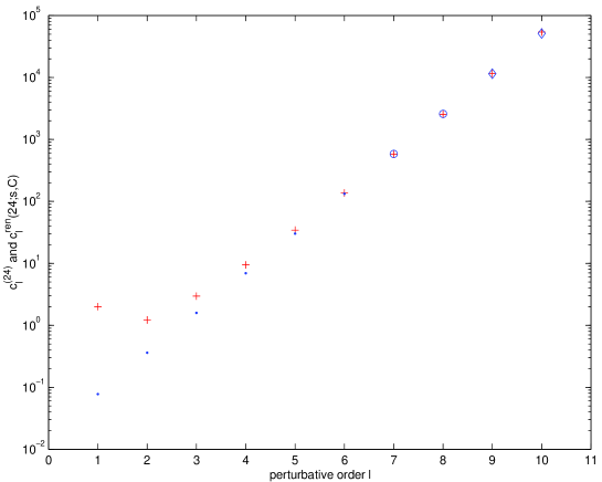
  Figure 1: The comparison between $c^{(24)}_{\ell}$ (red crosses) and $c^{ren}_{\ell}(24;s,C)$ as inferred from Fit1. The latter are marked as circles for the orders that have been taken into account in the fit; they are instead marked as dots or diamonds for other points. In particular diamonds can be looked at as forecasts for the two highest orders computed.

  Table 2: Perturbative coefficients $c^{ren}_{\ell}(M;s,C)$ as inferred from Fit1. $\delta_{M}$ are per cent deviations from the actual values of $c^{(M)}_{\ell}$. $\delta_{\infty}$ are the residual per cent deviations of $24^{4}$ coefficients with respect to infinite volume.

  	$M=8$	$\delta_{8}$	$M=24$	$\delta_{24}$	$\delta_{\infty}$
  $c^{ren}_{6}$	$1.30\cdot 10^{2}$	$-3\%$	$1.33\cdot 10^{2}$	$-3\%$	$<0.1\%$
  $c^{ren}_{7}$	$5.71\cdot 10^{2}$	$+1\%$	$5.84\cdot 10^{2}$	$+1\%$	$-0.1\%$
  $c^{ren}_{8}$	$2.51\cdot 10^{3}$	$+1\%$	$2.58\cdot 10^{3}$	$+2\%$	$-0.1\%$
  $c^{ren}_{9}$	$1.11\cdot 10^{4}$	$-1\%$	$1.15\cdot 10^{4}$	$-1\%$	$-0.2\%$
  $c^{ren}_{10}$	$4.90\cdot 10^{4}$	$-7\%$	$5.13\cdot 10^{4}$	$-6\%$	$-0.3\%$

  In the previous formula the factor $x$ is a possible further change of scale (see later). We obtain a value for the the scale $s_{1}=0.0074$. In previous works by our group the fits were performed without referring to a change of scale in the integral. The matching from a continuum to the lattice scheme was obtained by a change of variable $\beta_{cont}=\beta_{latt}-r-{{r^{\prime}}\over{\beta_{latt}}}$. In terms of the notation of this work the result of the fit in [5] reads $s_{1}=0.0078$. The $5\%$ difference sets a rough order of magnitude for what one has to live with in this and the other comparisons that we make: one should always keep in mind that we are managing notations that differ by higher orders. Notice that this agreement is a first good message for our understanding of finite size effects based on our formula for $c^{ren}_{\ell}(M;s,C)$: since we now fit results both on the $8^{4}$ and on the $24^{4}$ lattices (while the results in [5] were based on $8^{4}$ alone) the parametric dependence on the lattice size $M$ is supposed to work pretty well (anyway see later for more definite statements). With respect to Eq (14) Beneke [2] made the point that the result $s_{1}=0.0078$ in [5] could for example be interpreted by matching to the $\overline{\rm MS}$ scheme and taking into account a further change of scale (the factor $x$ in Eq (14)). The latter amounts to computing the $\overline{\rm MS}$ coupling at a scale $0.706/a$ instead of $\pi/a$. With the second (standard) choice of scale one obtains the standard result $\Lambda_{\overline{\rm MS}}=28.8\,\Lambda_{latt}$. $s_{1}=0.0078$ could in turn be interpreted as $0.706/\pi\times 1/28.8\,=0.0078$, while the result $s_{1}=0.0074$ could be read $0.666/\pi\times 1/28.8\,=0.0074$. One should not take all these considerations too seriously, e.g. there is no compelling commitment to the $\overline{\rm MS}$ scheme (once again, remember that one does not know which is the scheme in which our theoretical prejudice works the best). Still, it is reassuring that the numbers one gets are absolutely sensible as for their order of magnitude. Having made contact with our previous results, we now proceed to make contact with what we are mainly interested in, that is the new (ninth and tenth) orders. One can get a first glance at this by looking at Fig. (1) in which we compare the computed $c^{(24)}_{\ell}$ with the $c^{ren}_{\ell}(24;0.0074^{2},C^{(1)})$ (we will not quote the values obtained for the overall constant $C$ since they are not too enlightening). Notice that different symbols refer to different orders as far as the $c^{ren}_{\ell}(24;0.0074^{2},C^{(1)})$ are concerned: we want to emphasize the difference between the orders that are actually included in the fit and those that are looked at as forecasts to assess how well the asymptotic behaviour has been singled out. A very good agreement is manifest, which is actually magnified by the logarithmic scale. A careful inspection of the numbers themselves can be got from Table (2) in which we quote the values of the last five coefficients as inferred from Fit 1 on both lattice sizes. A first point to be made has to do with finite size effects. As we have already mentioned, a fit to data on both sizes is absolutely sensible and the deviations of the inferred coefficients from the actual ones are much the same on $8^{4}$ and on $24^{4}$. Notice also that the residual finite size effects between $24^{4}$ and infinite volume turn out to be negligible. As for the crucial issue of how well Fit 1 can single out the asymptotic behaviour we notice that the ninth coefficient is forecast with a precision of $1\%$, while a $6$–$7\%$ deviation is there for the tenth order. Notice also that, while orders seven and eight are kept into account in the fit, the agreement for orders less than seven results in a sensible shape for an asymptotic behaviour (by the way, the results are pretty stable to the inclusion of order six in the fit). This is the right time to make a point that specifies a statement that we have already made, i.e. that in inspecting the forecasts of our fits one should keep in mind that we are managing expressions that are there up to higher orders. This is of course not the end of the story. An equally important indetermination is coming from the fact that only a posteriori one can understand how asymptotic the expansion was at the highest order which has been taken into account in the fit. Roughly speaking, by fitting only the expansion for one quantity there is no obvious way to prevent the fit from pretending to have already reached the actual asymptotic regime.

• With respect to the last point we made there is a nice way to improve. We exploit it in what we call Fit 2. This time we make use of the fact that in [1] results for the first eight orders were computed not only for the $1\times 1$ Wilson loop (the basic plaquette), but also for the $2\times 2$.

  

  Figure 2: The comparison between $c^{(8)}_{\ell}$ (red crosses) and $c^{ren}_{\ell}(8;s,C)$ as inferred from Fit2. Same notations as in Fig. (1).

  Table 3: Perturbative coefficients $c^{ren}_{\ell}(M;s,C)$ as inferred from Fit2. Same notations as in Tab. (2).

  	$M=8$	$\delta_{8}$	$M=24$	$\delta_{24}$	$\delta_{\infty}$
  $c^{ren}_{6}$	$1.23\cdot 10^{2}$	$-10\%$	$1.25\cdot 10^{2}$	$-10\%$	$<0.1\%$
  $c^{ren}_{7}$	$5.51\cdot 10^{2}$	$-2\%$	$5.64\cdot 10^{2}$	$-2\%$	$-0.1\%$
  $c^{ren}_{8}$	$2.48\cdot 10^{3}$	$+0.2\%$	$2.55\cdot 10^{3}$	$+0.3\%$	$-0.1\%$
  $c^{ren}_{9}$	$1.12\cdot 10^{4}$	$-0.2\%$	$1.16\cdot 10^{4}$	$+0.2\%$	$-0.2\%$
  $c^{ren}_{10}$	$5.09\cdot 10^{4}$	$-3\%$	$5.31\cdot 10^{4}$	$-2\%$	$-0.3\%$

  Now, the IR Renormalon dominance is supposed to force a universal asymptotic behaviour. That’s why we now fit the formula for $c^{ren}_{\ell}(M;s,C^{(i)})$ to the set $\{c^{(8)}_{6},c^{(8)}_{7},c^{(8)}_{8},\\ c^{(8,2\times 2)}_{6},c^{(8,2\times 2)}_{7},c^{(8,2\times 2)}_{8}\}$. The $c^{(8,2\times 2)}_{\ell}$ are taken from [1], while of course this time a couple of different overall constant $C^{(i)}$ have to be fitted, corresponding to $i=1\times 1$ and $i=2\times 2$. Notice that this time, as an extra test of the control on finite size effects, we make use only of $8^{4}$ results for the basic plaquette. The value fitted for the scale is now $s_{1}=0.0065$. While we are still stopping at eight order in what we take into account for the fit, the curvature in the growth of the $2\times 2$ coefficients is opposite to that of $1\times 1$ and this corrects a bit with respect to Fit 1. As for the $12\%$ change in the scale, much the same that has already been told holds: while there is in a sense extra information on what has to be understood as asymptotic, it is nevertheless reassuring that the change in the coefficients is quite smooth and absolutely sensible as we are managing asymptotic behaviours. Not surprisingly, one can inspect from Fig. (2) (this time we plot the comparison for coefficients on the $8^{4}$ lattice) and (even better) from Table (3) that we have fairly improved the asymptotic behaviour. In particular, deviations for the forecasts on order ten are reduced to $1$–$2\%$, while other nice features like the consistency of finite size effects are still there. Also the residual finite size effects dependency turns out to be just the same (negligible) order.

• One can of course devise a fit in which all the information at hand is taken into account. This is what we proceed to do in what we refer to as Fit 3. This time we fit the formula for $c^{ren}_{\ell}(M;s,C^{(i)})$ to the set $\{c^{(8)}_{6},c^{(8)}_{7},c^{(8)}_{8},c^{(8)}_{9},c^{(8)}_{10},c^{(24)}_{6},c^{(24)}_{7},c^{(24)}_{8},c^{(24)}_{9},c^{(24)}_{10},c^{(8,2\times 2)}_{6},\\ c^{(8,2\times 2)}_{7},c^{(8,2\times 2)}_{8}\}$.

  

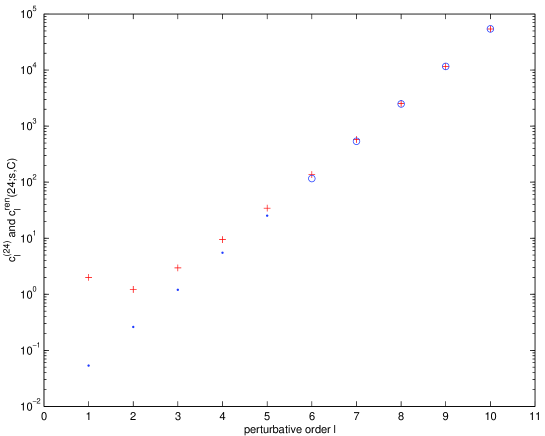
  Figure 3: The comparison between $c^{(24)}_{\ell}$ (red crosses) and $c^{ren}_{\ell}(24;s,C)$ as inferred from Fit3. Same notations as in Fig. (1). Notice that this time there are no diamonds.

  Table 4: Perturbative coefficients $c^{ren}_{\ell}(M;s,C)$ as inferred from Fit3. Same notations as in Tab. (2).

  	$M=8$	$\delta_{8}$	$M=24$	$\delta_{24}$	$\delta_{\infty}$
  $c^{ren}_{6}$	$1.14\cdot 10^{2}$	$-17\%$	$1.16\cdot 10^{2}$	$-17\%$	$<0.1\%$
  $c^{ren}_{7}$	$5.26\cdot 10^{2}$	$-7\%$	$5.37\cdot 10^{2}$	$-7\%$	$-0.1\%$
  $c^{ren}_{8}$	$2.43\cdot 10^{3}$	$-2\%$	$2.49\cdot 10^{3}$	$-2\%$	$-0.1\%$
  $c^{ren}_{9}$	$1.12\cdot 10^{4}$	$+0.2\%$	$1.16\cdot 10^{4}$	$+0.4\%$	$-0.2\%$
  $c^{ren}_{10}$	$5.21\cdot 10^{4}$	$<0.1\%$	$5.43\cdot 10^{4}$	$+0.5\%$	$-0.3\%$

  We are again changing the players on the ground by including a wide range of orders on both lattice sizes, together with information from $2\times 2$ Wilson Loop as well. The resulting scale is now $s_{1}=0.0056$, with a change with respect to Fit 2 which is again the same order of magnitude as that obtained in going from Fit 1 to Fit 2. The result is remarkably stable with respect to keeping into account only the last three orders for the basic plaquette (as for the $2\times 2$ Wilson Loop one can at the same time keep into account only the last order available, that is order eight). Results of the fit are plotted in Fig. (3) for the $24^{4}$ lattice and summarized in Table (4). Of course, this time it does not make any sense to compare with Fit 1 and Fit 2 as for the accuracy with which high orders are described.

In the end, what one can state is that going from Fit 1 to Fit 3 one is not going to jeopardize the overall picture: the transition in describing the growth of the coefficients is quite smooth, consistent with the asymptotic behaviour being better and better described. Again, one is validating the finite size effects as embedded in our formulae.

3.2 Finite size effects

From all the previous arguments the impact of finite size effects has already been widely discussed. Still, we think it is worthwhile to present the tests of finite size effects also in a graphical format. In Fig. (4) we depict something that has to do with finite size effects as resulting from the results of Fit 2.

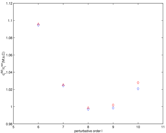
Figure 4: The ratios ${c^{(8)}_{\ell}}/{c^{ren}_{\ell}(8;s,C)}$ (red triangles pointing up and red diamonds) and ${c^{(24)}_{\ell}}/{c^{ren}_{\ell}(24;s,C)}$ (blue diamonds) as inferred from the results of Fit 2.

To be definite, we plot the ratios ${c^{(8)}_{\ell}}/{c^{ren}_{\ell}(8;0.0065^{2},C^{(1\times 1)})}$ and ${c^{(24)}_{\ell}}/{c^{ren}_{\ell}(24;0.0065^{2},C^{(1\times 1)})}$. One can directly see the conclusion that has already been drawn in the main discussion of Fit 2. While only the $8^{4}$ lattice has been taken into account in the fit, the points for both lattices fall on top of each other, i.e. from a fit to $8^{4}$ and the dependence on $M$ embedded in our formulae we describe basically with the same accuracy the coefficients of the $24^{4}$ lattice as well. Something similar is shown in Fig. (5) which is the same plot for the equivalent of Fit 3 in which only the $8^{4}$ lattice has been taken into account.

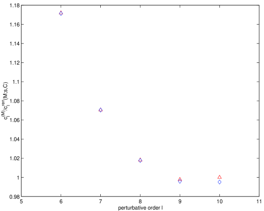
Figure 5: Same quantities as in Fig. (4) as obtained by the results of the equivalent of Fit 3 in which only $8^{4}$ lattice has been taken into account. Quantities for $8^{4}$ are plotted as red triangles pointing up while quantities for $24^{4}$ are plotted as blue diamonds.

4 Conclusions and perspectives

We computed the perturbative expansion of the basic $SU(3)$ plaquette on both a $8^{4}$ and a $24^{4}$ lattices to $\beta^{-10}$ order. We are now in a position to strengthen the claim in [1, 5], i.e. the coefficients growth is consistent with both the leading IR Renormalon dominance and with finite size effects on top of that. The latter does not exceed $4\%$ at the order we got and the residual finite size effects on the $24^{4}$ results are no more than half a percent, again at tenth order. Having verified that our previous analysis in [5] had neither failed in the extraction of the leading asymptotic behaviour nor underestimated finite size effects on the perturbative coefficients, these results make even more important to refine the analysis contained in the same paper as for the extraction of a quadratic contribution to the lattice representative for the Gluon Condensate. This refinement will now benefit by a control on finite size effects. This is what we plan to do in a near future [7], maybe going even through a further refinement on errors in the perturbative coefficients.

Appendix

We now sketch the steps to go from Eq. (9) to Eq. (10). As we have already said in Sec. (2.2) one way to treat the dependence on $s$ is to rescale the integration variable (define $t^{2}\equiv sk^{2}$). In this way one ends up with the rescaling $Q^{2}\rightarrow sQ^{2}$. This in turns means $\beta\rightarrow\beta(sQ^{2})$ which makes contact with the formulation of [1, 5] (again, as already said): $\beta\rightarrow\beta-r$ (at this level one obtains a one loop formula). We chose another way to proceed which manipulates the integrand in another way. By going through the change of variable of Eq. (5) one obtains (up to overall constants)

$$\int_{0}^{z_{ir}(M)}dz\;e^{-\beta z}\;(z_{0}-z)^{-1-\gamma}{{1}\over{1+6b_{0}{{z_{0}}\over{z_{0}-z}}{{1}\over{\beta}}\ln s}}\,,$$

$z_{ir}(M)$ being the value for $z$ pertaining to the IR cut–off $Q_{0}(M)$. The last factor is simply ${{\alpha_{\sf s}(sk^{2})}\over{\alpha_{\sf s}(k^{2})}}$. By expanding the latter in a geometric series (we are aiming at an expansion in $\beta^{-1}$) and by performing a change of variable we end up with

$$\beta^{\gamma}e^{-\beta z_{0}}(-1)^{-1-\gamma}\sum_{n}(6b_{0}z_{0}\ln s)^{n}\int_{-\beta z_{0}}^{\beta z_{ir}(M)-\beta z_{0}}e^{-z}z^{-1-\gamma-n}dz$$

Note that the effect of the scale $s$ propagates to high orders much the same way the leading logs expansion for $\alpha_{\sf s}$ is responsable for the Renormalon growth, i.e. via a geometric series. The last input is now the asymptotic expansion for incomplete $\Gamma$ functions (which is useful once one splits the previous integral in terms of a sum of incomplete $\Gamma$ functions)

$$\int_{z}^{\infty}dt\,e^{-t}\,t^{a-1}\approx z^{a-1}e^{-z}\sum_{k\geq 0}{{\Gamma(k+1-a)}\over{\Gamma(1-a)}}(-z)^{-k}$$

Once this expansion (valid for $|z|\rightarrow\infty$ in $|\arg z|<3\pi/2$) is plugged in, one proceeds to the final power expansion in $\beta^{-1}$ (which is easy to manage for example in $Mathematica^{\copyright}$).

References

- [1] F. Di Renzo, G. Marchesini and E. Onofri, Nucl. Phys. B 457, 202 (1995).
- [2] For a recent review and a complete listing of classical references see M. Beneke, Physics Reports 317, 1 (1999).
- [3] F. Di Renzo, G. Marchesini and E. Onofri, Nucl. Phys. B 497, 435 (1997).
- [4] See for example B. Allés, M. Campostrini, A. Feo and H. Panagopoulos, Phys. Lett. B 324, 443 (1994) and references therein.
- [5] G. Burgio, F. Di Renzo, G. Marchesini and E. Onofri, Phys. Lett. B 422, 98 (1998).
- [6] M.N. Chernodub, F.V. Gubarev, M.I. Polikarpov and V.I. Zakharov, Phys. Lett. B 475, 303 (2000) and references therein.
- [7] G. Burgio, F. Di Renzo and L. Scorzato, in preparation.
- [8] R. Alfieri, F. Di Renzo, E. Onofri and L. Scorzato, Nucl. Phys. B 578, 383 (2000).
- [9] F. Di Renzo and L. Scorzato, in preparation.