CERN-TH-2000/175

DESY-00-090

Effective Chiral Lagrangians and Lattice QCD

Jochen Heitger^a, Rainer Sommer^a and Hartmut Wittig^b,
a DESY
Platanenallee 6, D-15738 Zeuthen, Germany
^b CERN, Theory Division,
CH-1211 Geneva 23, Switzerland
Abstract

We propose a general method to obtain accurate estimates for some of the “low-energy constants” in the one-loop effective chiral Lagrangian by means of simulating lattice QCD. In particular, the method is sensitive to those constants whose values are required to test the hypothesis of a massless up-quark. Initial tests performed in the quenched approximation confirm that good statistical precision can be achieved. As a byproduct we obtain an accurate estimate for the ratio of pseudoscalar decay constants, $F_{\rm K}/F_{\pi}$, in the quenched approximation, which lies 10% below the experimental result. The quantities that serve to extract the low-energy constants also allow a test of the scaling behaviour of different discretizations of QCD and a search for the effects of dynamical quarks.

June 2000

1 Introduction

Chiral Perturbation Theory (ChPT) [?,?] plays an important rôle in the study of low-energy phenomena in QCD. As is well known, ChPT is based on simultaneous expansions of scattering amplitudes or hadronic matrix elements in powers of momentum and the quark masses $m_{{\rm u}},\,m_{{\rm d}}$ and $m_{{\rm s}}$, and the form of the effective chiral Lagrangian is entirely determined by chiral symmetry. Another feature is the emergence of a number of coupling constants at every given order, which incorporate the non-perturbative dynamics of QCD. These couplings – sometimes called “low-energy constants” – are a priori undetermined and can be fixed through phenomenological constraints in conjunction with additional assumptions. Currently the typical accuracy which is achieved in the determination of the low-energy constants is not very high (for a review, see [?]).

It has been noted some time ago that the mass parameters $m_{{\rm u}},\,m_{{\rm d}}$ and $m_{{\rm s}}$ cannot be fixed unambiguously from symmetry considerations alone. The reason is that the effective chiral Lagrangian is invariant under a family of transformations of the quark masses, which can be absorbed into the low-energy constants [?]. In particular, this hidden symmetry of the chiral Lagrangian implies that one cannot distinguish between $m_{{\rm u}}=0$ and $m_{{\rm u}}\approx 5\,{\rm MeV}$, whilst preserving all other phenomenological predictions. Thus, additional theoretical input beyond ChPT is required to decide whether $m_{{\rm u}}=0$ is indeed realized in nature. An obvious strategy is then to sharpen the current estimates for the low-energy constants and check whether they are compatible with the condition that $m_{{\rm u}}=0$.

Since $m_{{\rm u}}=0$ represents a simple solution to the strong CP problem, this question has continued to attract a lot of attention, despite several plausible arguments, each of which independently rules out $m_{{\rm u}}=0$ [?,?]. However, the problem has never been studied in a first principles approach starting from the QCD Lagrangian directly.

In this paper we propose and test a method to determine a large set of low-energy constants with good accuracy using lattice simulations. Given its technical feasibility, such an approach eliminates the use of theoretical assumptions in the specification of the chiral Lagrangian. In the context of testing $m_{{\rm u}}=0$ the rôle of lattice calculations has recently been discussed by Cohen, Kaplan and Nelson [?]. We expand on their proposal by incorporating the information gained by studying the mass dependence of matrix elements in addition to that of the pseudoscalar masses. Furthermore, we present ready-to-use numerical procedures which increase the statistical precision and discuss the influence of lattice artefacts. The latter point is of great relevance because the effective chiral Lagrangian of Gasser and Leutwyler is not valid for non-zero lattice spacing.

Our method is generally applicable in simulations of QCD with or without dynamical quarks. This initial study mainly serves to test its accuracy and limitations, and for that purpose it is sufficient to apply it to lattice data obtained in the quenched approximation. As a consequence we also consider comparisons of our lattice data with the quenched version of ChPT, thereby extracting some of the low-energy constants relevant for the quenched theory.

On the basis of our lattice data we conclude that the mass dependence of matrix elements can be determined with high precision in lattice simulations. Furthermore we show that low-energy constants in the chiral Lagrangian can be obtained with a typical, absolute statistical accuracy of $\pm\,0.05$ in the continuum limit. Systematic uncertainties due to neglected higher orders are estimated to be $\pm\,0.2$. However, a systematic study of the influence of higher orders in the chiral expansions has so far not been performed, owing to limitations in the range of light quark masses that one is currently able to explore. Future calculations at smaller quark masses will be required in order to settle this point.

The remainder of this paper is organized as follows. In Section 2 we recall the main concepts of ChPT. Our computational strategy is described in Section 3, and the numerical details are discussed in Section 4, focusing on the extrapolations to the continuum. Our results are presented in Section 5, and Section 6 contains some concluding remarks. Two appendices list some details about expressions in partially quenched ChPT and explain our choice of additional low-energy constants in the quenched theory.

2 Chiral perturbation theory

In this section we repeat the main features of ChPT and specify our notation. In addition to standard ChPT we also discuss its quenched and partially quenched versions.

2.1 Standard ChPT and $m_{{\rm u}}=0$

The effective chiral Lagrangian is written as a low-energy expansion [?,?]

$${\cal L}_{\rm eff}={\cal L}_{\rm eff}^{(2)}+{\cal L}_{\rm eff}^{(4)}+\ldots$$ (2.1)

The leading contribution ${\cal L}_{\rm eff}^{(2)}$ contains two coupling constants $F_{0}$ and $B_{0}$. To lowest order $F_{0}$ coincides with the pion decay constant $F_{\pi}$. Throughout this paper we adopt a convention in which $F_{\pi}\approx 93\,{\rm MeV}$. At order $p^{4}$ additional couplings $\alpha_{1},\alpha_{2},\ldots,\alpha_{12}$ appear in the effective chiral Lagrangian . These couplings are not constrained by chiral symmetry. Furthermore they contain the divergences that arise if one goes beyond tree level and thus depend on the renormalization scale (and scheme). As mentioned in the introduction, experimental information at low energies is not sufficient to specify the values of the complete set of couplings $\alpha_{1},\ldots,\alpha_{12}$. For this reason one has to add further theoretical constraints, which usually involve certain assumptions, such as large-$N_{\rm c}$ arguments. By applying such a procedure, the “standard” values of the low-energy constants in our convention for $N_{\rm f}=3$ flavours read [?,?,?,?,?,?,?]

$$\begin{array}[]{lcl}\alpha_{1}=\phantom{-}0.2\pm 0.4&&\alpha_{6}=-0.5\pm 0.4\\ \alpha_{2}=\phantom{-}1.07\pm 0.4&&\alpha_{7}=-0.5\pm 0.25\\ \alpha_{3}=-4.4\pm 1.4&&\alpha_{8}=\phantom{-}0.76\pm 0.4\\ \alpha_{4}=-0.76\pm 0.6&&\alpha_{9}=\phantom{-}7.8\pm 0.8\\ \alpha_{5}=\phantom{-}0.5\pm 0.6&&\alpha_{10}=-6.1\pm 0.8.\end{array}$$ (2.7)

Here the $\alpha_{i}$’s have been renormalized at scale $\mu=4\pi{F_{\pi}}$, which will always be used in the remainder of this paper. The constants $\alpha_{11}$ and $\alpha_{12}$ are of little phenomenological interest and are not included here.

The question whether $m_{{\rm u}}=0$ has been discussed at length in the literature [?,?,?,?]. The usual starting point is the observation that simultaneous transformations of the quark masses

$$m_{{\rm u}}^{\lambda}=m_{{\rm u}}+\lambda m_{{\rm d}}m_{{\rm s}},\quad m_{{\rm d}}^{\lambda}=m_{{\rm d}}+\lambda m_{{\rm s}}m_{{\rm u}},\quad m_{{\rm s}}^{\lambda}=m_{{\rm s}}+\lambda m_{{\rm u}}m_{{\rm d}},$$ (2.8)

and coupling constants according to

$$\alpha_{6}^{\lambda}=\alpha_{6}+\lambda\frac{(4\pi F_{0})^{2}}{4B_{0}},\quad\alpha_{7}^{\lambda}=\alpha_{7}+\lambda\frac{(4\pi F_{0})^{2}}{4B_{0}},\quad\alpha_{8}^{\lambda}=\alpha_{8}-\lambda\frac{(4\pi F_{0})^{2}}{2B_{0}},$$ (2.9)

leaves the effective chiral Lagrangian invariant. Here, $\lambda$ denotes an arbitrary parameter, and for $\lambda\not=0,\,m_{{\rm u}}=0$ one can generate an effective up-quark mass such that all predictions by ChPT, in particular for ratios of quark masses, remain unchanged. In order to test whether $m_{{\rm u}}=0$ one has to determine the linear combination [?] $(2\alpha_{8}-\alpha_{5})$, which, however, is not directly accessible from phenomenology. The value of $\alpha_{5}$ is obtained from the ratio of kaon to pion decay constants, $F_{\rm K}/F_{\pi}$, but $\alpha_{8}$ can only be inferred from the linear combination

$$\alpha_{5}-12\alpha_{7}-6\alpha_{8},$$ (2.10)

which is related to the Gell-Mann–Okubo formula. Clearly this linear combination is invariant under the transformation of eq. (2.9). As pointed out in [?] a choice for $\alpha_{7}$ and $\alpha_{8}$ which is compatible with $m_{{\rm u}}=0$ is given by

$$m_{{\rm u}}=0:\quad\alpha_{8}=-0.9\pm 0.4,\quad\alpha_{7}=0.25\pm 0.25,$$ (2.11)

which is quite different from the corresponding numbers listed in eq. (2.7). The task for lattice simulations is now to provide independent determinations of $\alpha_{5},\,\alpha_{8}$ from linear combinations which are not invariant under eq. (2.9), starting from the QCD Lagrangian. Provided that these estimates turn out to be sufficiently accurate, it should then be possible to test the hypothesis that $m_{{\rm u}}=0$.

2.2 Partially quenched ChPT

The rôle of lattice simulations for the determination of the $\alpha_{i}$’s has already been stressed in [?,?], and most recently in [?]. In particular, it has been noted that simulations of “partially quenched” QCD, in which the sea and valence quarks can be chosen independently, may be useful as well as technically feasible. Thus, one is not forced to simulate at the physical values of the ${\rm u}$, ${\rm d}$ and ${\rm s}$ quarks. Instead, the only requirement is that the pseudoscalar masses be small compared with the typical chiral scale of $\Lambda_{\chi}\approx 1\,{\rm GeV}$. Hence the use of moderately light sea and valence quark masses and their independent variation may be sufficient to extract the low-energy constants.

It has to be kept in mind, though, that the values of the $\alpha_{i}$’s have to be determined separately for $N_{\rm f}=2$ and 3 flavours of dynamical quarks. This is a relevant point since there is currently not much experience with simulation algorithms for odd numbers of flavour.

Partially quenched ChPT has been studied to O$(p^{4})$ by a number of authors [?,?,?]. Here we focus on the one-loop expressions for pseudoscalar masses and decay constants obtained by Sharpe [?] for $N_{\rm f}$ degenerate flavours of sea quarks. For the remainder of this paper we also take over some of the notation used in that reference. In particular, we denote the mass of the sea quark by $m_{S}$, whereas the masses of the (in general non-degenerate) valence quarks are denoted by $m_{1},\,m_{2}$. As in [?] we introduce the dimensionless parameters

$$y_{ij}=\frac{B_{0}(m_{i}+m_{j})}{(4\pi F_{0})^{2}},\qquad i,\,j\in\{1,\,2,\,S\}.$$ (2.12)

By setting $\Lambda_{\chi}=4\pi F_{0}$ in eqs. (14) and (18) of ref. [?], we obtain the generic formulae for the pseudoscalar mass and decay constant, i.e.

$$m_{\rm PS}^{2} = y_{12}(4\pi F_{0})^{2}\bigg{\{}1+\frac{1}{N_{\rm f}}\left[\frac{y_{11}(y_{SS}-y_{11})\ln{y_{11}}-y_{22}(y_{SS}-y_{22})\ln{y_{22}}}{y_{22}-y_{11}}\right]$$ (2.13)

$$+y_{12}(2\alpha_{8}-\alpha_{5})+y_{SS}N_{\rm f}(2\alpha_{6}-\alpha_{4})\bigg{\}}$$

$$\frac{F_{\rm PS}}{F_{0}} = 1-\frac{N_{\rm f}}{4}\left(y_{1S}\ln{y_{1S}}+y_{2S}\ln{y_{2S}}\right)$$ (2.14)

$$+\frac{1}{2N_{\rm f}}\left(\frac{y_{11}y_{22}-y_{SS}y_{12}}{y_{22}-y_{11}}\ln\frac{y_{11}}{y_{22}}+y_{12}-y_{SS}\right)$$

$$+y_{12}\frac{1}{2}\alpha_{5}+y_{SS}\frac{N_{\rm f}}{2}\alpha_{4}.$$

Here the constants $\alpha_{i}$ are to be evaluated at scale $\mu=\Lambda_{\chi}=4\pi F_{0}\approx 1170\,{\rm MeV}$. These expressions will later be used to form quantities that allow for the extraction of the $\alpha_{i}$’s using lattice data.

2.3 Quenched ChPT

Quenched ChPT has originally been discussed in refs. [?,?]. The complete chiral Lagrangian to order $p^{4}$ in quenched QCD has been studied by Colangelo and Pallante [?]. Their results form the basis of our analysis.

As is well known flavour singlets have to be treated differently in the quenched approximation: the decoupling of the $\eta^{\prime}$ from the pseudoscalar octet by means of the anomaly is not realized in the quenched theory. Therefore, the quenched chiral Lagrangian contains additional low-energy constants associated with flavour-singlet contributions. These include the singlet mass scale $m_{0}$ and the coupling constant $\alpha_{\Phi}$, which multiplies the kinetic term of the singlet field in the quenched chiral Lagrangian. The mass scale $m_{0}$ is usually expressed in terms of the parameter $\delta$ defined by

$$\delta=\frac{m_{0}^{2}}{3(4\pi F_{0})^{2}}.$$ (2.15)

From various lattice studies (e.g. [?,?,?,?]) one expects $\delta\approx 0.1$. For $\alpha_{\Phi}$ the available estimates have been summarized in [?] as $\alpha_{\Phi}\approx 0.6$.

Following ref. [?] we restrict ourselves to the case of degenerate quarks. The complete results at one loop for the pseudoscalar mass and decay constant read 

$$m_{\rm PS}^{2} = y\,(4\pi F_{0})^{2}\left\{1-\left(\delta-\textstyle\frac{2}{3}\alpha_{\Phi}{y}\right)\left[1+\ln{y}\right]+\left((2\alpha_{8}^{\rm q}-\alpha_{5}^{\rm q})-\frac{\alpha_{\Phi}}{3}\right)y\right\}$$ (2.16)

$$\frac{F_{\rm PS}}{F_{0}} = 1+y\,\textstyle\frac{1}{2}\alpha_{5}^{\rm q}.$$ (2.17)

Here $y$ is defined as

$$y=\frac{2B_{0}m}{(4\pi F_{0})^{2}},$$ (2.18)

and $\alpha_{8}^{\rm q},\,\alpha_{5}^{\rm q}$ denote the analogues of the low-energy constants $\alpha_{8}$ and $\alpha_{5}$ in the quenched theory.

3 Strategy

We now introduce the procedure to determine the low-energy constants from lattice data by studying the quark mass dependence of suitably defined ratios of pseudoscalar masses and matrix elements. In particular it is useful to investigate the mass dependence around some reference quark mass $m_{\rm ref}$. It is important to realize that this reference point does not have to coincide with a physical quark mass [?]. We only require that it should lie inside the range of simulated quark masses and within the domain of applicability of ChPT.

3.1 The ratios $R_{\rm M}$ and $R_{\rm F}$

Let us consider the case of degenerate valence quarks, $m_{1}=m_{2}=m$, either in the quenched approximation or in partially quenched QCD at a fixed value of the sea quark mass $m_{S}$. If we introduce

$$y=\frac{2B_{0}m}{(4\pi F_{0})^{2}},\quad y_{\rm ref}=\frac{2B_{0}m_{\rm ref}}{(4\pi F_{0})^{2}},\quad x=y/y_{\rm ref},$$ (3.19)

then the ratios defined by

$$R_{\rm M}(x) = \left(\frac{F_{\rm PS}(y)}{G_{\rm PS}(y)}\right)\left/\left(\frac{F_{\rm PS}(y_{\rm ref})}{G_{\rm PS}(y_{\rm ref})}\right)\right.$$ (3.20)

$$R_{\rm F}(x) = F_{\rm PS}(y)\left/F_{\rm PS}(y_{\rm ref})\right.$$ (3.21)

are universal functions of the parameter $x$, which measures the deviation from the reference point $y_{\rm ref}$. Here, $G_{\rm PS}$ denotes the matrix element of the pseudoscalar density between a pseudoscalar state and the vacuum, and the arguments of $F_{\rm PS},\,G_{\rm PS}$ refer to the quark mass value at which the matrix elements have to be evaluated. Using the definition of the current quark mass in terms of $F_{\rm PS},\,G_{\rm PS}$ and $m_{\rm PS}$ (see, for instance, eqs. (2.1) and (2.2) in ref. [?]), eq. (3.20) can be rewritten as

$$R_{\rm M}(x)=\left(\frac{2y}{m_{\rm PS}^{2}(y)}\right)\left/\left(\frac{2y_{\rm ref}}{m_{\rm PS}^{2}(y_{\rm ref})}\right)\right.=x\,\frac{m_{\rm PS}^{2}(y_{\rm ref})}{m_{\rm PS}^{2}(y)}.$$ (3.22)

Extracting the low-energy constants from the ratios $R_{X},\,X={\rm M,\,F}$ instead of the masses and matrix elements themselves has several advantages:

• The ratios $R_{X}$ can be computed with high statistical precision owing to the strong correlations between numerator and denominator;

• The renormalization factors of the axial current and the pseudoscalar density drop out in $R_{\rm M}$ and $R_{\rm F}$. The ratios can therefore be readily extrapolated to the continuum limit, so that all dependence on the lattice spacing is eliminated. Strictly speaking it is only in the continuum limit that one is justified to compare the predictions of ChPT with lattice data;

• Since discretization errors are under good control in $R_{X}$ the effects of dynamical quarks can be isolated unambiguously.

The high level of statistical accuracy of the ratios is crucial in order not to compromise the precision in the continuum limit. Extracting the low-energy constants from the $x$-dependence in the continuum limit in turn guarantees that these estimates will not be distorted by cutoff effects.

The simple renormalization and high precision of the ratios may also be exploited to perform scaling tests for different fermionic discretizations.

3.2 Expressions for $R_{\rm M}$ and $R_{\rm F}$ in ChPT

Below we give a list with the expressions for $R_{\rm M}$ and $R_{\rm F}$ in quenched and partially quenched ChPT. For simplicity we restrict ourselves to the case of degenerate valence quarks. The case of non-degenerate valence quarks in partially quenched ChPT is discussed in detail in Appendix A.

Note that we have not yet specified the reference point $y_{\rm ref}$. At this stage the precise definition of its numerical value is not needed, and we thus postpone its specification to Section 5, where we describe our numerical results.

We begin by considering $R_{\rm M}$ and $R_{\rm F}$ in quenched ChPT. By inserting eq. (2.16) into eq. (3.22) we obtain

$$R_{\rm M}^{\rm q}(x)=\frac{1-(\delta-\frac{2}{3}\alpha_{\Phi}y_{\rm ref})(1+\ln y_{\rm ref})+y_{\rm ref}[(2\alpha_{8}^{\rm q}-\alpha_{5}^{\rm q})-\frac{\alpha_{\Phi}}{3}]}{1-(\delta-\frac{2}{3}\alpha_{\Phi}xy_{\rm ref})(1+\ln(xy_{\rm ref}))+xy_{\rm ref}[(2\alpha_{8}^{\rm q}-\alpha_{5}^{\rm q})-\frac{\alpha_{\Phi}}{3}]}.$$ (3.23)

Provided that all masses and couplings are small, it is allowed to expand the denominator, which gives

$$R_{\rm M}^{\rm q}(x) = 1+\delta\ln{x}-\textstyle\frac{2}{3}\alpha_{\Phi}y_{\rm ref}\left[x\ln{x}+(x-1)(\textstyle\frac{1}{2}+\ln y_{\rm ref})\right]$$ (3.24)

$$-y_{\rm ref}(x-1)(2\alpha_{8}^{\rm q}-\alpha_{5}^{\rm q}).$$

Similarly we obtain

$$R_{\rm F}^{\rm q}(x)=\frac{1+xy_{\rm ref}{1\over 2}\alpha_{5}^{\rm q}}{1+y_{\rm ref}{1\over 2}\alpha_{5}^{\rm q}},$$ (3.25)

which, after expanding the denominator, becomes

$$R_{\rm F}^{\rm q}(x)=1+y_{\rm ref}(x-1){1\over 2}\alpha_{5}^{\rm q}.$$ (3.26)

In partially quenched ChPT it is useful to always define the reference point $y_{\rm ref}$ at

$$m_{1}=m_{2}=m_{S}=m_{\rm ref},\quad y_{\rm ref}=\frac{2B_{0}m_{\rm ref}}{(4\pi F_{0})^{2}}.$$ (3.27)

There are several possibilities to study the mass dependence of the ratios $R_{X}$. Let us first consider the case of equal sea and valence quark masses. The $x$-dependent part in $R_{X}$ is then obtained by setting

$$\hbox{SS:}\quad m_{1}=m_{2}=m_{S}=xm_{\rm ref},$$ (3.28)

which will be labelled “SS” in the following. By taking the appropriate limits in eqs. (2.12) and (2.13) for the above choices of quark masses and inserting the resulting expressions into the definition of $R_{\rm M}$, we obtain, after expanding the denominator:

$$R_{\rm M}^{\rm SS}(x) = 1-\frac{1}{N_{\rm f}}y_{\rm ref}\left[x\ln{x}+(x-1)\ln{y_{\rm ref}}\right]$$ (3.29)

$$-y_{\rm ref}(x-1)\left[(2\alpha_{8}-\alpha_{5})+N_{\rm f}(2\alpha_{6}-\alpha_{4})\right].$$

For $R_{\rm F}$ the corresponding result is

$$R_{\rm F}^{\rm SS}(x)=1-\frac{N_{\rm f}}{2}y_{\rm ref}\left[x\ln{x}+(x-1)\ln y_{\rm ref}\right]+y_{\rm ref}(x-1)\textstyle\frac{1}{2}\left(\alpha_{5}+N_{\rm f}\alpha_{4}\right).$$ (3.30)

For $m_{1},\,m_{2}\not=m_{S}$ the $x$-dependence can be mapped out using either the valence or the sea quarks. In the former case, which we label “VV” we define the $x$-dependent part through

$$\hbox{VV:}\quad m_{1}=m_{2}=xm_{\rm ref},\quad m_{S}=m_{\rm ref}$$ (3.31)

instead of eq. (3.28), which leads to the expressions

$$R_{\rm M}^{\rm VV}(x) = 1-\frac{1}{N_{\rm f}}y_{\rm ref}\left[(2x-1)\ln{x}+2(x-1)\ln y_{\rm ref}\right]$$ (3.32)

$$-y_{\rm ref}(x-1)\left[(2\alpha_{8}-\alpha_{5})+\textstyle\frac{1}{N_{\rm f}}\right]$$

$$R_{\rm F}^{\rm VV}(x) = 1-\frac{N_{\rm f}}{4}y_{\rm ref}\left[(x+1)\ln\left(\textstyle\frac{1}{2}(x+1)\right)+(x-1)\ln y_{\rm ref}\right]$$ (3.33)

$$+y_{\rm ref}(x-1)\textstyle\frac{1}{2}\alpha_{5}.$$

A comparison of the expressions for $R_{\rm M}$ and $R_{\rm F}$ for the “SS” and “VV” cases shows that they are sensitive to different linear combinations of low-energy constants, depending on whether the $x$-dependence is defined using eq. (3.28) or eq. (3.31). In particular, we find that it is possible to extract directly from $R_{\rm M}^{\rm VV}(x)$ the linear combination $(2\alpha_{8}-\alpha_{5})$, which is relevant to the question of whether $m_{{\rm u}}=0$.

There are several other possibilities to define the dependence of $R_{X}$ on the quark masses, also allowing for non-degenerate valence quarks. Details are listed in Appendix A.

3.3 Extracting the low-energy constants

We now describe a method to determine the low-energy constants from the ratios $R_{X}$ in the quenched and unquenched cases. To this end we choose two values of mass parameters, $x_{1},\,x_{2}$, and introduce the quantity

$$\Delta R_{X}(x_{1},x_{2})=R_{X}(x_{1})-R_{X}(x_{2}),\quad x_{1}<x_{2},\quad X={\rm M,\,F}.$$ (3.34)

By inserting the expressions for the ratios $R_{X}$ we can easily solve for the low-energy constants. For instance, from eqs. (3.26) and (3.34) we find

$$\alpha_{5}^{\rm q}=2\frac{\Delta R_{\rm F}^{\rm q}(x_{1},x_{2})}{(x_{1}-x_{2})y_{\rm ref}}.$$ (3.35)

Similar combinations of the $\alpha_{i}$’s can be obtained in partially quenched QCD. The explicit expressions are given in Appendix A, and one can easily convince oneself that they serve to determine $\alpha_{4},\,\alpha_{5},\,\alpha_{6}$ and $\alpha_{8}$.

The quantity $\Delta R_{\rm M}^{\rm q}$ is a special case, since it also depends on the low-energy constants $\delta$ and $\alpha_{\Phi}$, which only occur in the quenched theory. However, by inserting the estimates for $\delta$ and $\alpha_{\Phi}$ quoted in the literature we can solve for $(2\alpha_{8}^{\rm q}-\alpha_{5}^{\rm q})$, i.e.

$$(2\alpha_{8}^{\rm q}-\alpha_{5}^{\rm q}) = \left\{y_{\rm ref}(x_{1}-x_{2})\right\}^{-1}\times\Big{\{}\delta\ln({x_{1}}/{x_{2}})-\Delta R_{\rm M}^{\rm q}(x_{1},x_{2})$$ (3.36)

$$-\textstyle\frac{2}{3}\alpha_{\Phi}y_{\rm ref}\left[x_{1}\ln{x_{1}}-x_{2}\ln{x_{2}}+(x_{1}-x_{2})\left(\textstyle\frac{1}{2}+\ln y_{\rm ref}\right)\right]\Big{\}}.$$

The expressions for $R_{X}$ themselves can also be used in order to extract the low-energy constants from least-$\chi^{2}$ fits over a suitably chosen interval in $x$. The differences $\Delta R_{X}$, however, have the advantage that some of the lattice artefacts may cancel. Thus, instead of first extrapolating $R_{X}$ to the continuum limit and then forming the differences $\Delta R_{X}$, one may compute $\Delta R_{X}(x_{1},x_{2})$ at non-zero lattice spacing and then perform the continuum extrapolation. Obviously the results must be independent of the ordering of the two procedures, which offers an additional check against the influence of lattice artefacts. By contrast, if a fitting procedure is employed at non-zero lattice spacing then it is a priori not clear whether the continuum expressions for the ratios $R_{X}$ are valid.

Our method to extract the low-energy constants is only viable if there is sufficient overlap between the region of validity of ChPT and the range of quark masses accessible in current lattice simulations. On present computers it is not possible to simulate very light quarks without suffering from large finite-volume effects. Furthermore, the fermion action and lattice spacings employed in this work do not allow the use of quark masses which are below approximately half of the strange quark mass. The reason is the occurrence of “exceptional configurations” [?,?], which correspond to unphysical zero modes of the lattice Dirac operator. Therefore, since one is restricted to a range of relatively large quark masses, one must check the results against the influence of higher orders in the chiral expansion: if large, these would modify the numerical estimates for the low-energy constants considerably. This will be discussed in more detail in Section 5.

4 Continuum limit of $R_{X}$ and $\Delta R_{X}$

The ratios $R_{X}$ have been computed using the same quenched configurations as in our earlier papers [?,?]. Results for hadron and current quark masses, as well as for $F_{\rm PS}$ and $F_{\rm PS}/G_{\rm PS}$ are listed in Table 1 of ref. [?]. Details of our numerical procedures are described in Appendix A of the same paper. Here we only mention that non-perturbative ${\rm O}(a)$ improvement [?,?,?] has been employed, and we will therefore assume that the remaining discretization errors are of order $a^{2}$.

In contrast to our earlier papers the statistical errors in this work have been estimated using a bootstrap procedure [?], with 200 bootstrap samples generated from the sets of gauge configurations. This allows us to keep a constant number of bootstrap samples at every value of the bare coupling, regardless of the number of configurations. By performing the continuum extrapolation of $R_{X}(x)$ for every bootstrap sample, our error procedure thus preserves the correlations in the mass parameter $x$. Throughout this paper we quote the symmetrized error from the central 68% of the bootstrap distribution.

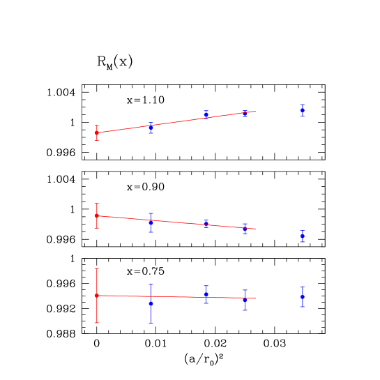
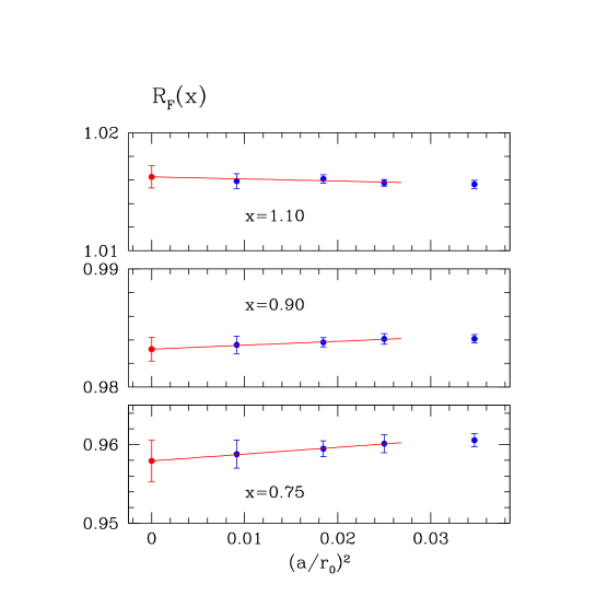
Figure 1: Continuum extrapolations of $R_{\rm M}(x)$ and $R_{\rm F}(x)$ for selected values of the mass parameter $x$.

The value of the reference quark mass $m_{\rm ref}$ is defined through the condition

$$\left(m_{\rm PS}r_{0}\right)^{2}\Big{|}_{m=m_{\rm ref}}=3,$$ (4.37)

a choice that has also been considered in refs. [?,?]. For $F_{0}=F_{\pi}=93.3\,{\rm MeV}$ the numerical value of $y_{\rm ref}$ is thus $y_{\rm ref}=0.3398\ldots$. Lattice data for the hadronic radius $r_{0}$ [?] have been taken from ref. [?]. For $r_{0}=0.5\,{\rm fm}$ the definition of eq. (4.37) corresponds to a pseudoscalar meson whose squared mass is roughly twice as large as the kaon mass squared, and therefore $m_{\rm ref}\approx m_{{\rm s}}$ (with “s” standing for “strange”). The results for $F_{\rm PS}$ and $F_{\rm PS}/G_{\rm PS}$ obtained for several values of the bare coupling have been interpolated in the current quark mass $m$ to common values of $x=m/m_{\rm ref}$. To this end the two neighbouring points which straddle the value of $x$ were used in a linear interpolation. If $x$ was slightly outside the range of simulated quark masses, a linear extrapolation was performed using the three nearest points. The stability of this procedure was checked by varying the input masses and/or performing quadratic interpolations/extrapolations. Our sets of simulated quark masses cover the range $0.75\leq{x}\leq 1.4$, and we have chosen increments of 0.05 to map out the mass dependence of $R_{X}(x)$.

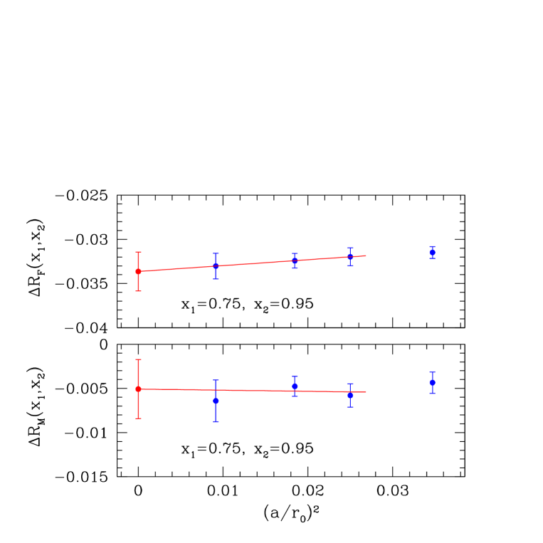
Figure 2: Continuum extrapolations of $\Delta R_{\rm M}$ and $\Delta R_{\rm F}$.

In Fig. 1 we plot the ratios $R_{\rm M}(x)$ and $R_{\rm F}(x)$ against $(a/r_{0})^{2}$ for three different values of $x$. The plots show that lattice artefacts are very small in general and are consistent with leading cutoff effects of order $a^{2}$. As a safeguard against higher-order lattice artefacts, we have excluded the points computed for our coarsest lattice ($a\approx 0.1\,{\rm fm}$) from the extrapolation. Results obtained by performing the extrapolations for all four values of the lattice spacing were entirely consistent, albeit with a smaller statistical error.

At non-zero lattice spacing the statistical precision is better than 0.3% and 0.2% for $R_{\rm M}$ and $R_{\rm F}$, respectively. In the continuum limit these figures are only slightly larger, namely 0.4% for $R_{\rm M}$ and 0.3% for $R_{\rm F}$. This demonstrates the high level of precision that can be achieved in the continuum limit. Furthermore it is clear that the extrapolation is well controlled.

As mentioned in Section 3 the results for $\Delta R_{X}$ in the continuum limit can be obtained either directly from the continuum values of $R_{X}$ or from a continuum extrapolation of $\Delta R_{X}$ computed at non-zero lattice spacing. The latter extrapolations are shown in Fig. 2 for a particular choice of $x_{1}$ and $x_{2}$. As in the case of the ratios $R_{X}$ themselves the continuum limit is easy to control.

5 Results

We can now compare our results for the ratios $R_{X}$ to the expressions predicted by ChPT. Since the numerical data have been obtained in the quenched approximation, we will focus on the determination of $\alpha_{5}^{\rm q}$ and $(2\alpha_{8}^{\rm q}-\alpha_{5}^{\rm q})$.

5.1 Low-energy constants in quenched ChPT

The determination of $\alpha_{5}^{\rm q}$ from eq. (3.35) is straightforward, since it only depends on the mass parameters $x_{1}$ and $x_{2}$. However, in order to compute $(2\alpha_{8}^{\rm q}-\alpha_{5}^{\rm q})$ from eq. (3.36) one must make a suitable choice of $\delta$ and $\alpha_{\Phi}$. Here we are going to consider two cases, namely

Q1: $$\delta=0.12\pm 0.02,\quad\alpha_{\Phi}=0$$ (5.38)

Q2: $$\delta=0.05\pm 0.02,\quad\alpha_{\Phi}=0.5.$$ (5.39)

The reasoning which led us to consider these two distinct sets of parameters is described in Appendix B.

Our estimates for $\alpha_{5}^{\rm q}$ and $(2\alpha_{8}^{\rm q}-\alpha_{5}^{\rm q})$ have been obtained from $\Delta R_{\rm F}(x_{1},x_{2})$ and $\Delta R_{\rm M}(x_{1},x_{2})$ for $x_{1}=0.75$ and $x_{2}=0.95$. This choice was motivated by the desire to go to the smallest possible quark masses, whilst maintaining a reasonably large $x$-interval in order to check the stability of the results against variations in the parameters $x_{1}$ and $x_{2}$. Following this procedure, we obtained the following estimates for the low-energy constants in quenched ChPT

$$\alpha_{5}^{\rm q} = 0.99\pm 0.06$$ (5.40)

$$(2\alpha_{8}^{\rm q}-\alpha_{5}^{\rm q}) = \left\{\begin{array}[]{lr}0.35\pm 0.05\pm 0.07;&\quad\hbox{Q1}\\ 0.02\pm 0.05\pm 0.07;&\quad\hbox{Q2}\end{array}.\right.$$ (5.43)

Here, the first error is statistical, while the second (where quoted) is due to the variation of $\pm 0.02$ in the value of $\delta$ for both parameter sets Q1 and Q2. These results can now be inserted into the expressions for the ratios $R_{\rm M}$ and $R_{\rm F}$, eqs. (3.24) and (3.26), respectively, and the resulting curves are compared with the data in Fig. 3 (a)–(c).

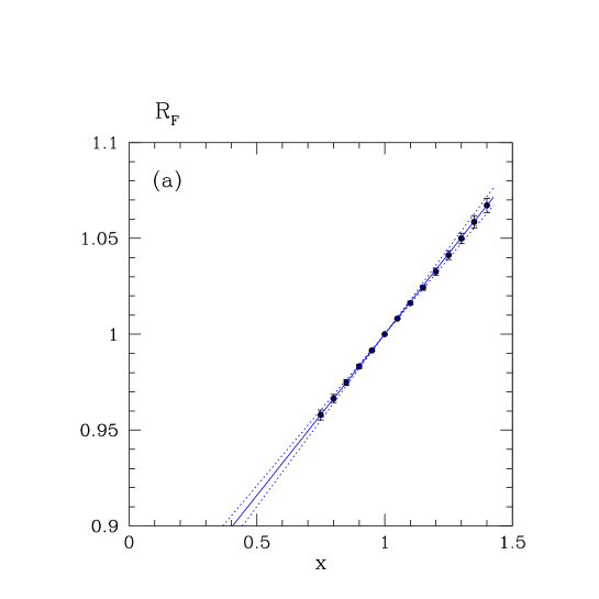
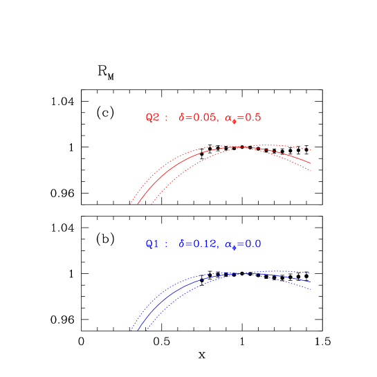
Figure 3: (a): Data for the ratio $R_{\rm F}$ compared with the curve obtained by inserting the low-energy constant of eq. (5.40); (b) and (c): the same for the ratio $R_{\rm M}$ using the low-energy constants of eq. (5.43) for parameter sets Q1 and Q2, respectively. Dotted lines indicate the variation due to the statistical uncertainty in the extraction of the low-energy constants.

The linearity of $R_{\rm F}$ predicted by one-loop quenched ChPT is well reproduced by the numerical data, resulting in very stable estimates for $\alpha_{5}^{\rm q}$. Although the result in eq. (5.40) has been extracted from a fairly narrow $x$-interval, it provides a good representation of the data over the entire range of quark masses considered here. The determination of $(2\alpha_{8}^{\rm q}-\alpha_{5}^{\rm q})$ is also quite stable for both sets of values of $\delta,\,\alpha_{\Phi}$, i.e. Q1 and Q2. In both cases a good description of the numerical data is achieved for $x\;\raisebox{-2.58334pt}{$\stackrel{{\scriptstyle\textstyle{<}}}{{\sim}}$}\;1.2$, with $(2\alpha_{8}^{\rm q}-\alpha_{5}^{\rm q})$ extracted for Q1 tracing the data quite well even at the largest $x$-values.

Estimates for $\alpha_{5}^{\rm q}$ and $(2\alpha_{8}^{\rm q}-\alpha_{5}^{\rm q})$ obtained from the continuum extrapolations of $\Delta R_{\rm F}$ and $\Delta R_{\rm M}$ shown in Fig. 2 are entirely consistent with eqs. (5.40) and (5.43). The same is true if the low-energy constants are extracted directly from fits to $R_{X}(x)$ for $x$ in the interval $0.75\leq{x}\leq 0.95$; the results are numerically almost identical to those obtained using the differences $\Delta R_{X}$.

5.2 Effects of higher orders in the quark mass

Although the results presented in the last subsection suggest that the one-loop formulae for quenched ChPT offer a good description of the $x$-dependence of the ratios $R_{X}$, further work is needed to corroborate these findings by extending the range of quark masses under study to smaller values. For instance, the downward curvature observed in the prediction for $R_{\rm M}$ when $x<0.75$ remains to be verified.

Furthermore, data at smaller quark masses will be required to systematically assess the influence of higher-order terms in the chiral expansion on the determination of the low-energy constants. Such terms manifest themselves in additional contributions proportional to $x^{2}$ in the formulae for $R_{X}$. Since the range $0.75\leq{x}\leq 0.95$ corresponds to pseudoscalar meson masses between 590 and $670\,{\rm MeV}$, it cannot be excluded that higher-order terms have a sizeable impact on the extraction of the $\alpha_{i}$’s.

Even without results at smaller masses there are several possibilities to study the effects of neglecting higher orders in ChPT on our estimates for $\alpha_{5}^{\rm q}$ and $(2\alpha_{8}^{\rm q}-\alpha_{5}^{\rm q})$. We stress, however, that none of the methods described below can replace the systematic investigation of smaller quark masses.

An obvious way to proceed is to add a quadratic term to the expressions for $R_{\rm F}^{\rm q}$ and $R_{\rm M}^{\rm q}$. For instance, the modified expression for $R_{\rm F}^{\rm q}$ reads

$$R_{\rm F}^{\rm q}(x)\longrightarrow 1+y_{\rm ref}(x-1)\textstyle\frac{1}{2}\alpha_{5}^{\rm q}+y_{\rm ref}^{2}(x^{2}-1)\,d_{\rm F},$$ (5.44)

with a similar quadratic term proportional to $d_{\rm M}$ in the case of $R_{\rm M}^{\rm q}$. One can now perform least-$\chi^{2}$ fits over the entire range $0.75\leq{x}\leq 1.4$, thereby extracting the low-energy constants as well as $d_{\rm F},\,d_{\rm M}$. Because of the linearity of the data for $R_{\rm F}$ the only effect of including $x^{2}$-terms in the determination of $\alpha_{5}^{\rm q}$ is to increase its statistical error to $\pm\,0.19$. The estimates for $(2\alpha_{8}^{\rm q}-\alpha_{5}^{\rm q})$ are more sensitive: compared with eqs. (5.43) their central values increase by 0.11 and 0.22 for the parameter sets Q1 and Q2, respectively, while the statistical error is increased to $\pm\,0.12$. The variation in the central values, or the larger statistical error in the case of $\alpha_{5}^{\rm q}$, may serve as an estimate of the uncertainty induced by neglecting higher orders.

An alternative, albeit naive, estimate of the effect in question is obtained by assuming that the chiral expansion converges like a geometric series. This implies that one expects the quadratic contributions to $R_{X}$ to be roughly as large as the square of the linear ones. Here we consider $R_{\rm F}^{\rm q}$ as the generic case, since it does not involve logarithmic terms. Its linear contribution amounts to $\approx 16\%$ at $x=1$, so that the quadratic term is estimated as $0.025\,x^{2}$. If we generalize this estimate, then the systematic uncertainty in $\Delta R_{X}(x_{1},x_{2})$ due to neglecting quadratic terms is given by

$$\hbox{syst. error in}\;\Delta R_{X}(x_{1},x_{2})\approx\pm\,0.025\,(x_{1}^{2}-x_{2}^{2}).$$ (5.45)

Through eqs. (3.35) and (3.36) this is easily translated into systematic errors on $\alpha_{5}^{\rm q}$ and $(2\alpha_{8}^{\rm q}-\alpha_{5}^{\rm q})$, as

$$\hbox{syst. error in}\;\alpha_{5}^{\rm q} \approx \pm\,0.25$$ (5.46)

$$\hbox{syst. error in}\;(2\alpha_{8}^{\rm q}-\alpha_{5}^{\rm q}) \approx \pm\,0.13,$$ (5.47)

which is of the same order of magnitude as the previous estimate.

Finally one can compare the expanded and unexpanded expressions for $R_{\rm M}$ and $R_{\rm F}$, which differ at order $x^{2}$ (cf. eqs. (3.23)–(3.26)). By extracting the low-energy constants from least-$\chi^{2}$ fits to the ratios in eqs. (3.23) and (3.25) we obtain yet another set of results. For $\alpha_{5}^{\rm q}$ the central value is larger by 20%, whereas the result for $(2\alpha_{8}^{\rm q}-\alpha_{5}^{\rm q})$ remains essentially unchanged.

In order to present a synthesis of the various efforts to estimate the uncertainty due to neglecting higher orders, we note that the typical size of this systematic error amounts to $\pm\,0.2$ for both $\alpha_{5}^{\rm q}$ and $(2\alpha_{8}^{\rm q}-\alpha_{5}^{\rm q})$.

5.3 Application: the ratio $F_{\rm K}/F_{\pi}$

The result for $\alpha_{5}^{\rm q}$ extracted from $R_{\rm F}^{\rm q}$ can be used to compute the ratio of the decay constants of the kaon and pion, $F_{\rm K}/F_{\pi}$. In fact, one usually employs the reverse procedure by using the experimental result for $F_{\rm K}/F_{\pi}$ to extract the phenomenological value of $\alpha_{5}$.

If we assume that contributions proportional to differences in the valence quark masses can be neglected, we can simply use the definition of $R_{\rm F}^{\rm q}(x)$ to compute $F_{\rm K}/F_{\pi}$:

$$\frac{F_{\rm K}}{F_{\pi}}=\frac{R_{\rm F}^{\rm q}(x_{\rm K})}{R_{\rm F}^{\rm q}(x_{\pi})}=1+y_{\rm ref}(x_{\rm K}-x_{\pi})\textstyle\frac{1}{2}\alpha_{5}^{\rm q}.$$ (5.48)

Here the dimensionless mass parameters $x_{\rm K}$ and $x_{\pi}$ are related to the kaon and pion masses by

$$x_{\rm K}\,y_{\rm ref}=\frac{m_{\rm K}^{2}}{(4\pi F_{0})^{2}}=0.1782$$ (5.49)

$$x_{\pi}\,y_{\rm ref}=\frac{m_{\pi}^{2}}{(4\pi F_{0})^{2}}=0.0142,$$ (5.50)

where, as in ref. [?], we have used $m_{\rm K}=495\,{\rm MeV}$ and $m_{\pi}=139.6\,{\rm MeV}$. If the estimate for $\alpha_{5}^{\rm q}$ from eq. (5.40) is inserted we find

$$\frac{F_{\rm K}}{F_{\pi}}=1.081\pm 0.005\pm 0.017.$$ (5.51)

Here the first error is statistical and the second is the estimated uncertainty in $\alpha_{5}^{\rm q}$, due to neglecting quadratic terms. The above result is significantly smaller than the experimental value of ${F_{\rm K}}/{F_{\pi}}=1.22$ [?].

A formula for ${F_{\rm K}}/{F_{\pi}}$ in one-loop quenched ChPT, which also accounts for differences in the valence quark masses, can be derived from eqs. (18) and (20) of ref. [?]. The low-energy constant that appears in the one-loop counterterm is the same as in the quenched degenerate case [?,?]. In our notation the full one-loop expression for ${F_{\rm K}}/{F_{\pi}}$ reads

$$\frac{F_{\rm K}}{F_{\pi}} = 1+\,y_{\rm ref}(x_{\rm K}-x_{\pi})\,\frac{1}{2}\,\alpha_{5}^{\rm q}-\frac{1}{2}\left\{\left(\delta-\frac{\alpha_{\Phi}}{3}\,x_{\rm K}\,y_{\rm ref}\right)\right.$$ (5.52)

$$\left.-\,\frac{3\delta\,x_{\rm K}-\alpha_{\Phi}\,y_{\rm ref}x_{\pi}(2x_{\rm K}-x_{\pi})}{6(x_{\rm K}-x_{\pi})}\,\ln\left(\frac{2x_{\rm K}-x_{\pi}}{x_{\pi}}\right)\right\}.$$

Note that one recovers eq. (5.48) when $\delta=\alpha_{\Phi}=0$. For the two sets of parameters, Q1 and Q2, the results for ${F_{\rm K}}/{F_{\pi}}$ are evaluated as

$$\frac{F_{\rm K}}{F_{\pi}}=\left\{\begin{array}[]{ll}1.125\pm 0.005\pm 0.016\pm 0.007;&\hbox{Q1}\\ 1.110\pm 0.005\pm 0.017\pm 0.007;&\hbox{Q2}\end{array},\right.$$ (5.55)

where the additional third error is due to the variation of $\pm\,0.02$ in the input value for $\delta$. While contributions proportional to differences in the quark masses enhance the result for ${F_{\rm K}}/{F_{\pi}}$ compared with eq. (5.51), the value is still smaller than experiment by about 10 %. Deviations of this order of magnitude are typical of quantities computed in the quenched approximation. This has previously been inferred from calculations of the hadron spectrum [?,?], and the results presented here firmly establish these findings for matrix elements of local currents as well. The fact that ${F_{\rm K}}/{F_{\pi}}$ is typically underestimated in quenched calculations has been observed before [?,?]. Note, however, that our estimates have much smaller uncertainties than those quoted in the other references.

Finally we remark that the enhancement in the estimate of ${F_{\rm K}}/{F_{\pi}}$ due to differences in the quark masses, demonstrates that these effects can be quite significant if the quark mass difference is as large as that between the physical light and strange quarks. By contrast, estimates of these effects based on masses in the region of that of the strange quark tend to be much smaller [?,?].

5.4 Partially quenched ChPT

In addition to our analysis of the quenched version of ChPT we can also tentatively use the expressions for $R_{\rm M}$ and $R_{\rm F}$ which are derived in the partially quenched theory. This essentially serves two purposes. On the one hand we can investigate to what extent the ratios $R_{X}$ in quenched QCD are described by the formulae of partially quenched ChPT. If a severe mismatch is encountered it will signal that sea-quark effects are not accounted for. On the other hand, by extracting the $\alpha_{i}$’s using the expressions of partially quenched ChPT but quenched numerical data, we can test how much of the relevant physical information for the low-energy constants in full QCD is encoded in the mass dependence obtained in the quenched approximation. The subsequent calculation of quantities such as the ratio $F_{\rm K}/F_{\pi}$ and its comparison with experiment provides a quantitative criterion for this task. In this spirit we have investigated the cases labelled “SS” and “VV” discussed in Section 3.

If we employ the expression for $R_{\rm F}^{\rm SS}$, eq. (3.30), we find that the linearity of the numerical data is incompatible with the additional logarithmic terms contained in the formula. As a consequence an acceptable representation of the data for $R_{\rm F}$ cannot be achieved on the basis of eq. (3.30). We conclude that the mass dependence of the quenched decay constant is incompatible with the chiral behaviour predicted in full QCD!

By contrast, the expression for $R_{\rm M}^{\rm SS}$ fits the numerical data very well over almost the entire range in $x$. However, the disagreement between the data and $R_{\rm F}^{\rm SS}$ indicates that the “SS” formulae cannot be applied to the quenched data in any reasonable manner. Therefore, we refrain from quoting an estimate for $(2\alpha_{8}-\alpha_{5})+3(2\alpha_{6}-\alpha_{4})$, even though a good modelling of the data for $R_{\rm M}$ can be achieved.

On the other hand, the expressions for both ratios obtained for the “VV” case do indeed lead to an acceptable representation of the data, at least for $x\;\raisebox{-2.58334pt}{$\stackrel{{\scriptstyle\textstyle{<}}}{{\sim}}$}\;1$. Quoting only statistical errors, the results for the low-energy constants read

$$\alpha_{5} = 0.75\pm 0.06$$ (5.56)

$$(2\alpha_{8}-\alpha_{5}) = 0.15\pm 0.05.$$ (5.57)

The curves corresponding to these values are shown in Fig. 4 (a) and (b). While for $x\;\raisebox{-2.58334pt}{$\stackrel{{\scriptstyle\textstyle{<}}}{{\sim}}$}\;1$ the curves fit the data quite well, they deviate much more at larger $x$ than the corresponding quenched ones. Compared with the quenched case, the results for the $\alpha_{i}$ are roughly in the same ball park.

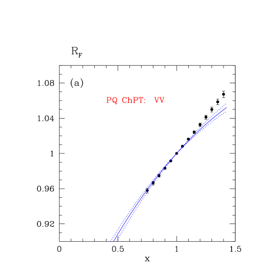
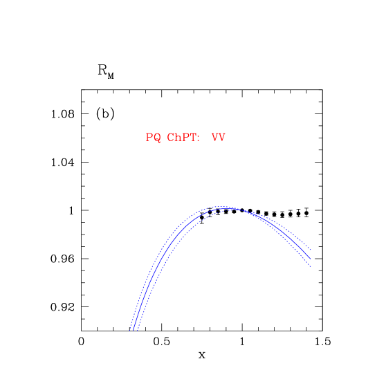
Figure 4: The “VV” case in partially quenched ChPT (a): data for the ratio $R_{\rm F}$ compared with the curve obtained by inserting the low-energy constant of eq. (5.56); (b): the same for the ratio $R_{\rm M}$ using the low-energy constants of eq. (5.57). Dotted lines indicate the variation due to the statistical uncertainty in the extraction of the low-energy constants.

Using the value for $\alpha_{5}$ extracted from $R_{\rm F}^{\rm VV}$ we can now compute the ratio ${F_{\rm K}}/{F_{\pi}}$. Since the low-energy constants in the partially quenched and full theories are the same, we have used the expression derived in full QCD [?]. In our notation it reads

$$\frac{F_{\rm K}}{F_{\pi}} = 1+y_{\rm ref}(x_{\rm K}-x_{\pi})\textstyle\frac{1}{2}\alpha_{5}$$ (5.58)

$$+\,\frac{y_{\rm ref}}{4}\bigg{\{}(3x_{\pi}-2x_{\rm K})\ln(x_{\pi}y_{\rm ref})-x_{\rm K}\ln(x_{\rm K}y_{\rm ref})$$

$$\left.-\frac{1}{2}(4x_{\rm K}-x_{\pi})\ln\left(\frac{4x_{\rm K}-x_{\pi}}{3x_{\pi}}\right)\right\}.$$

After inserting the numerical values for $x_{\rm K},x_{\pi},y_{\rm ref}$ and $\alpha_{5}$ one finds

$$\frac{F_{\rm K}}{F_{\pi}}=1.228\pm 0.005\,\hbox{(stat)}\pm 0.016.$$ (5.59)

Here the uncertainty of $\pm\,0.016$ is due to neglecting higher orders. This result is actually compatible with the experimental value, which is not entirely surprising, since our estimate of $\alpha_{5}=0.75(6)$ agrees quite well with its phenomenological value of $0.5\pm 0.6$ quoted in eq. (2.7). These findings suggest that the valence quark mass dependence of the numerically determined ratios $R_{X}$ in the region of the strange quark mass is only weakly distorted by neglecting dynamical quarks. The relevant quark mass effects which account for the difference between the quenched result eq. (5.55) and the experimental value $F_{\rm K}/F_{\pi}=1.22$, appear to be due to the very light up and down quarks in full QCD. Their non-linear effects can be efficiently accounted for by the formulae of partially quenched ChPT.

6 Summary and conclusions

In this paper we have proposed a general method to extract the low-energy constants in effective chiral Lagrangians by studying the mass dependence of suitably defined ratios of matrix elements and matching it to ChPT. The ratios are typically obtained with high statistical precision and can be extrapolated to the continuum limit in a straightforward manner. Thus, the method offers a conceptually clean way to determine the low-energy constants, since it is strictly speaking only in the continuum limit that a comparison of lattice data to ChPT can be performed.

The dimensionless ratios $R_{X}$ are also interesting in their own right: they can be used to study the scaling behaviour of different fermionic discretizations without having to compute renormalization factors. Furthermore, the effects of dynamical quarks can be isolated unambiguously, since lattice artefacts are under good control.

In this initial study we have presented results for the quenched approximation. The typical value of the absolute statistical error of $\pm\,0.05$ in the low-energy constants confirms that the achievable precision is indeed quite high compared with “conventional” phenomenological determinations. The main limitation at present is that results at smaller quark masses are not available. It is therefore not possible to systematically investigate whether there is sufficient overlap between the range of simulated quark masses and the domain of validity of ChPT. As a consequence the present estimated uncertainty of $\pm\,0.2$ in the low-energy constants due to higher-order terms are fairly coarse. It is expected, though, that the simulation of smaller quark masses will be feasible within the formulation of QCD with a “twisted” mass term (tmQCD) [?]. In this construction the mass parameter protects against unphysical zero modes of the Dirac operator, which alleviates the problem of exceptional configurations encountered in simulations with Wilson fermions. Initial studies have shown promising results, and it is planned to exploit this method further in the present context.

Returning to the problem of examining the question of whether $m_{{\rm u}}=0$, it is useful to recall that the problem can be solved through a reliable determination of $\alpha_{8}$. In the quenched approximation we obtain

$$\alpha_{8}^{\rm q}=\left\{\begin{array}[]{lr}0.67\pm 0.04\,\hbox{(stat)}\,\pm 0.04;&\quad\hbox{Q1}\\ 0.50\pm 0.04\,\hbox{(stat)}\,\pm 0.04;&\quad\hbox{Q2}\end{array},\right.$$ (6.62)

where the second error is due to the variation in $\delta$, and the additional uncertainty arising from neglecting higher orders is estimated to be $\pm\,0.2$. There is a priori no reason why the low-energy constant $\alpha_{8}^{\rm q}$ should be numerically close to its counterpart in the full theory, and hence it would surely be premature to give a full assessment of the problem on the basis of our quenched results. Nevertheless, it is interesting to note that our results for $\alpha_{8}^{\rm q}$ are quite close to the “standard” value for $\alpha_{8}$, eq. (2.7), which supports a non-vanishing up-quark mass. By contrast, given our data for the ratios $R_{X}$ it would be very difficult to accommodate a large negative value, which is required for the up-quark to be massless (see eq. (2.11)).

Finally we wish to add a few general comments on the philosophy of our approach. Provided that the quark masses used in simulations are small enough for the one-loop expressions of ChPT to apply, our procedures altogether avoid chiral extrapolations of lattice results, which are known to be quite difficult to control. The example of the computation of $F_{\rm K}/F_{\pi}$ shows that the problem can be separated in two parts. The information which involves quark masses near the chiral limit can be extracted safely in ChPT, whereas the mass dependence for masses in the region somewhat below the strange quark mass can be adequately studied in lattice QCD. The latter part is the additional theoretical input needed to determine some of the low-energy constants, which are not accessible from chiral symmetry considerations alone. In short, our method amounts to exploiting the complementary character of ChPT and lattice QCD. The applicability of ChPT itself can be tested once quark masses somewhat smaller than those in our present work become accessible.

The next step is the application of our method to the case of dynamical quarks. Here the relevant formulae that will be required are listed in Appendix A. Simulations using either the O$(a)$ improved Wilson action for $N_{\rm f}=2$ flavours of dynamical quarks [?] or other improvement schemes [?] have already been performed [?,?,?,?]. Whereas an analysis of those results will be able to treat the two-flavour case, the extension to the physically most interesting case of $N_{\rm f}=3$ flavours will require a significant amount of additional simulations. It is also worth investigating applications to the case of non-degenerate sea quarks and to try to determine the low-energy constant $\alpha_{7}$ [?]. However, the main message of this paper is the following. In order to settle the question of whether $m_{{\rm u}}=0$ one does not even require the same level of accuracy as that of the quenched results presented here. A satisfactory analysis of the problem in the case of three degenerate flavours is therefore quite a realistic prospect.

Acknowledgements. We are indebted to Gilberto Colangelo and Elisabetta Pallante for essential clarifications concerning the application of quenched ChPT. We are also grateful to Ruedi Burkhalter for useful correspondence. This work is part of the ALPHA Collaboration research programme. We thank DESY for allocating computer time on the APE/Quadrics computers at DESY-Zeuthen and the staff of the computer centre at Zeuthen for their support.

Appendix A Partially quenched ChPT – the general case

In this appendix we list the expressions for $R_{\rm M}$ and $R_{\rm F}$, as well as for $\Delta R_{\rm M}$ and $\Delta R_{\rm F}$, in partially quenched QCD. In particular we discuss all possibilities to define the $x$-dependence of $R_{X}$, allowing also for non-degenerate valence quarks.

We start by considering the expressions in eqs. (2.12)–(2.14). At the reference point we require all quark masses to coincide with $m_{\rm ref}$ (cf. eq. (3.27)). Two cases, labelled “SS” and “VV” have already been discussed in Section 3.2. In addition to “VV”, one can also study the $x$-dependence by varying the sea quark mass $m_{S}$ for fixed, degenerate valence quarks:

$$\hbox{SS2:}\quad m_{1}=m_{2}=m_{\rm ref},\quad m_{S}=xm_{\rm ref}.$$ (A.63)

For non-degenerate valence quarks one may define

VS1: $$m_{1}=xm_{\rm ref},\quad m_{2}=m_{S}=m_{\rm ref}$$ (A.64)

VS2: $$m_{1}=m_{\rm ref},\quad m_{2}=m_{S}=xm_{\rm ref}.$$ (A.65)

In order to list the expressions for $R_{\rm M}$ and $R_{\rm F}$ for all cases $\rm SS,\,VV,\ldots,VS2$ it is convenient to introduce the general parameterization

$$R_{\rm M}(x) = 1-\textstyle\frac{y_{\rm ref}}{N_{\rm f}}\rho_{\rm M}(x;y_{\rm ref})-y_{\rm ref}(x-1)\lambda_{\rm M}(\mathbf{\alpha})$$ (A.66)

$$R_{\rm F}(x) = 1-N_{\rm f}\,y_{\rm ref}\,\rho_{\rm F}(x;y_{\rm ref})-y_{\rm ref}(x-1)\lambda_{\rm F}(\mathbf{\alpha}).$$ (A.67)

Here, $\rho_{\rm M}$ and $\rho_{\rm F}$ are functions of $x$ and $y_{\rm ref}$, and $\lambda_{\rm M},\lambda_{\rm F}$ denote linear combinations of the low-energy constants. The expressions for $\rho$ and $\lambda$ are shown in Tables 1 and 2, respectively.

	$\rho_{\rm M}(x;y_{\rm ref})$	$\lambda_{\rm M}(\mathbf{\alpha})$
SS	$x\ln{x}+(x-1)\ln y_{\rm ref}$	$(2\alpha_{8}-\alpha_{5})+N_{\rm f}(2\alpha_{6}-\alpha_{4})$
VV	$(2x-1)\ln{x}+2(x-1)\ln y_{\rm ref}$	$(2\alpha_{8}-\alpha_{5})+\frac{1}{N_{\rm f}}$
SS2	$-(x-1)\ln y_{\rm ref}$	$N_{\rm f}(2\alpha_{6}-\alpha_{4})-\frac{1}{N_{\rm f}}$
VS1	$x\ln{x}+(x-1)\ln y_{\rm ref}$	$\frac{1}{2}(2\alpha_{8}-\alpha_{5})$
VS2	0	$\frac{1}{2}(2\alpha_{8}-\alpha_{5})+N_{\rm f}(2\alpha_{6}-\alpha_{4})$

Table 1: The functions $\rho$ and $\lambda$ for the ratio $R_{\rm M}(x)$.

	$\rho_{\rm F}(x;y_{\rm ref})$	$\lambda_{\rm F}(\mathbf{\alpha})$
SS	$\frac{1}{2}\left(x\ln{x}+(x-1)\ln y_{\rm ref}\right)$	$-\frac{1}{2}(\alpha_{5}+N_{\rm f}\alpha_{4})$
VV	$\frac{1}{2}\left(\frac{x+1}{2}\ln\frac{x+1}{2}+\frac{x-1}{2}\ln y_{\rm ref}\right)$	$-\frac{1}{2}\alpha_{5}$
SS2	$\frac{1}{2}\left(\frac{x+1}{2}\ln\frac{x+1}{2}+\frac{x-1}{2}\ln y_{\rm ref}\right)$	$-\frac{N_{\rm f}}{2}\alpha_{4}$
VS1	$\frac{1}{4}\left(\frac{x+1}{2}\ln\frac{x+1}{2}+\frac{x-1}{2}\ln y_{\rm ref}+\frac{1}{N_{\rm f}^{2}}\ln{x}\right)$	$-\frac{1}{4}(\alpha_{5}+\frac{1}{N_{\rm f}})$
VS2	$\frac{1}{4}\left(\frac{x+1}{2}\ln\frac{x+1}{2}+\frac{3(x-1)}{2}\ln y_{\rm ref}+\frac{N_{\rm f}^{2}-1}{N_{\rm f}^{2}}x\ln{x}\right)$	$-\frac{1}{4}\alpha_{5}-\frac{N_{\rm f}}{2}\alpha_{4}+\frac{1}{4N_{\rm f}}$

Table 2: The functions $\rho$ and $\lambda$ for the ratio $R_{\rm F}(x)$.

Using the functions $\rho_{X}$ and $\lambda_{X}$, $X={\rm M,\,F}$, it is now quite easy to solve for particular linear combinations of low-energy constants by considering the differences $\Delta R_{X}(x_{1},x_{2})$ introduced in eq. (3.34).

With these definitions the linear combinations of low-energy constants denoted by $\lambda_{X}(\mathbf{\alpha}),\,X={\rm M,\,F}$ are simply given by

$$\lambda_{\rm M}(\mathbf{\alpha}) = -\frac{\Delta R_{\rm M}(x_{1},x_{2})+\frac{y_{\rm ref}}{N_{\rm f}}\left(\rho_{\rm M}(x_{1},y_{\rm ref})-\rho_{\rm M}(x_{2},y_{\rm ref})\right)}{y_{\rm ref}(x_{1}-x_{2})}$$ (A.68)

$$\lambda_{\rm F}(\mathbf{\alpha}) = -\frac{\Delta R_{\rm F}(x_{1},x_{2})+{y_{\rm ref}}\,{N_{\rm f}}\left(\rho_{\rm F}(x_{1},y_{\rm ref})-\rho_{\rm F}(x_{2},y_{\rm ref})\right)}{y_{\rm ref}(x_{1}-x_{2})}.$$ (A.69)

By evaluating the right-hand side, using numerical data for $\Delta R_{X}$, one can easily solve for the desired combination of $\alpha_{i}$’s.

Appendix B Choices for $\delta$ and $\alpha_{\Phi}$

In this appendix we motivate our choices for the parameters $\delta$ and $\alpha_{\Phi}$ specified in eqs. (5.38) and (5.39). Here we will closely follow the analysis presented by the CP-PACS Collaboration [?], i.e. we consider the ratio

$$s=\frac{m_{\rm PS}^{2}(m_{1},m_{2})}{m_{1}+m_{2}}\cdot\frac{2m_{1}}{m_{\rm PS}^{2}(m_{1},m_{1})}\times\frac{m_{\rm PS}^{2}(m_{1},m_{2})}{m_{1}+m_{2}}\cdot\frac{2m_{2}}{m_{\rm PS}^{2}(m_{2},m_{2})},$$ (B.70)

where the arguments in $m_{\rm PS}^{2}$ have been included in order to distinguish between degenerate and non-degenerate mesons. By inserting the expressions for $m_{\rm PS}^{2}$ in quenched ChPT for degenerate and non-degenerate quarks (cf. eq. (9) in [?]) one obtains after expanding the denominator

$$s=1+\delta\left(2-\frac{y_{11}+y_{22}}{y_{11}-y_{22}}\ln\frac{y_{11}}{y_{22}}\right)+\frac{\alpha_{\Phi}}{3}\left(-(y_{11}+y_{22})+2y_{11}\frac{y_{22}}{y_{11}-y_{22}}\ln\frac{y_{11}}{y_{22}}\right).$$ (B.71)

In ref. [?] the quantity $t$ was defined as

$$t=2-\frac{y_{11}+y_{22}}{y_{11}-y_{22}}\ln\frac{y_{11}}{y_{22}}.$$ (B.72)

For $\alpha_{\Phi}=0$ eq. (B.71) reduces to a simple, linear relation between $s$ and $t$:

$$s=1+\delta\cdot{t},$$ (B.73)

with the slope given by $\delta$. By plotting the numerically determined values for the ratio $s$ against $t$ for $\alpha_{\Phi}=0$, CP-PACS concluded that all their data were enclosed within the “wedge” defined by $\delta=0.08$–0.12. This wedge is represented in Fig. 5 by the solid lines.

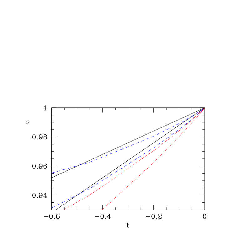
Figure 5: The “wedges” defined through eq. (B.71) for different values of $\delta$ and $\alpha_{\Phi}$ as explained in the text.

So far the parameter $\alpha_{\Phi}$ has not been considered in this kind of analysis. We are now going to argue that a value of $\alpha_{\Phi}\approx 0.5$, as suggested by Sharpe in [?], is only compatible with the CP-PACS data enclosed by the solid wedge, if $\delta$ is chosen in the range $0.03$–0.07. To this end we identify $m_{1}=m_{{\rm s}}$, so that $y_{11}=0.343$. The mass ratio $y_{11}/y_{22}$ is then varied between 1 and 24.4, where the latter number is the value of $2m_{{\rm s}}/(m_{{\rm u}}+m_{{\rm d}})$ computed in standard ChPT [?]. For $\delta=0.08$–0.12, $\alpha_{\Phi}=0$ one thus recovers the wedge denoted by the solid line in Fig. 5, which encloses the CP-PACS data.

If one combines $\delta=0.08$–0.12 with the independent estimate of $\alpha_{\Phi}=0.5$ from [?] one obtains instead the wedge defined by the dotted lines, which is clearly incompatible with CP-PACS’s numerical data. Agreement can only be restored if $\delta$ is lowered. The dashed curves, which correspond to $\delta=0.03$–0.07, $\alpha_{\Phi}=0.5$, are again consistent with the wedge defined by the solid lines. These observations lead us to consider the two sets of parameters as specified in eqs. (5.38) and (5.39).

References

- [1] J. Gasser and H. Leutwyler, Ann. Phys. 158 (1984) 142.
- [2] J. Gasser and H. Leutwyler, Nucl. Phys. B250 (1985) 465.
- [3] J. Bijnens, G. Ecker and J. Gasser, hep-ph/9411232, (1994).
- [4] D.B. Kaplan and A.V. Manohar, Phys. Rev. Lett. 56 (1986) 2004.
- [5] H. Leutwyler, Nucl. Phys. B337 (1990) 108.
- [6] H. Leutwyler, hep-ph/9609465, (1996).
- [7] A.G. Cohen, D.B. Kaplan and A.E. Nelson, JHEP 11 (1999) 027, hep-lat/9909091.
- [8] J. Bijnens and F. Cornet, Nucl. Phys. B296 (1988) 557.
- [9] J. Bijnens, Nucl. Phys. B337 (1990) 635.
- [10] C. Riggenbach, J. Gasser, J.F. Donoghue and B.R. Holstein, Phys. Rev. D43 (1991) 127.
- [11] D. Babusci et al., Phys. Lett. B277 (1992) 158.
- [12] S. Sharpe and N. Shoresh, Nucl. Phys. B (Proc. Suppl.) 83-84 (2000) 968, hep-lat/9909090.
- [13] S. Sharpe and N. Shoresh, hep-lat/0006017, (2000).
- [14] S.R. Sharpe, Phys. Rev. D56 (1997) 7052, hep-lat/9707018.
- [15] M.F.L. Golterman and K.C. Leung, Phys. Rev. D57 (1998) 5703, hep-lat/9711033.
- [16] C.W. Bernard and M.F.L. Golterman, Phys. Rev. D46 (1992) 853, hep-lat/9204007.
- [17] S.R. Sharpe, Phys. Rev. D46 (1992) 3146, hep-lat/9205020.
- [18] G. Colangelo and E. Pallante, Nucl. Phys. B520 (1998) 433, hep-lat/9708005.
- [19] Y. Kuramashi, M. Fukugita, H. Mino, M. Okawa and A. Ukawa, Phys. Rev. Lett. 72 (1994) 3448.
- [20] T. Bhattacharya and R. Gupta, Phys. Rev. D54 (1996) 1155, hep-lat/9510044.
- [21] CP-PACS Collaboration, S. Aoki et al., Phys. Rev. Lett. 84 (2000) 238, hep-lat/9904012.
- [22] W. Bardeen, A. Duncan, E. Eichten and H. Thacker, Nucl. Phys. B (Proc. Suppl.) 83-84 (2000) 215, hep-lat/9909128.
- [23] S.R. Sharpe, Nucl. Phys. B (Proc. Suppl.) 53 (1997) 181, hep-lat/9609029.
- [24] G. Colangelo and E. Pallante, private communication.
- [25] ALPHA & UKQCD Collaborations, J. Garden, J. Heitger, R. Sommer and H. Wittig, Nucl. Phys. B571 (2000) 237, hep-lat/9906013.
- [26] S. Sint and P. Weisz, Nucl. Phys. B502 (1997) 251, hep-lat/9704001.
- [27] M. Lüscher, S. Sint, R. Sommer, P. Weisz and U. Wolff, Nucl. Phys. B491 (1997) 323, hep-lat/9609035.
- [28] W. Bardeen, A. Duncan, E. Eichten, G. Hockney and H. Thacker, Phys. Rev. D57 (1998) 1633, hep-lat/9705008.
- [29] ALPHA Collaboration, M. Guagnelli, J. Heitger, R. Sommer and H. Wittig, Nucl. Phys. B560 (1999) 465, hep-lat/9903040.
- [30] B. Sheikholeslami and R. Wohlert, Nucl. Phys. B259 (1985) 572.
- [31] M. Lüscher, S. Sint, R. Sommer and P. Weisz, Nucl. Phys. B478 (1996) 365, hep-lat/9605038.
- [32] B. Efron, SIAM Review 21 (1979) 460.
- [33] UKQCD Collaboration, K.C. Bowler et al., hep-lat/9910022, (1999).
- [34] R. Sommer, Nucl. Phys. B411 (1994) 839, hep-lat/9310022.
- [35] ALPHA Collaboration, M. Guagnelli, R. Sommer and H. Wittig, Nucl. Phys. B535 (1998) 389, hep-lat/9806005.
- [36] C. Caso et al., Eur. Phys. J. C3 (1998) 1.
- [37] M.F.L. Golterman and K.C. Leung, Phys. Rev. D56 (1997) 2950, hep-lat/9702015.
- [38] F. Butler, H. Chen, J. Sexton, A. Vaccarino and D. Weingarten, Nucl. Phys. B421 (1994) 217, hep-lat/9310009.
- [39] CP-PACS Collaboration, R. Burkhalter et al., Nucl. Phys. B (Proc. Suppl.) 73 (1999) 3, hep-lat/9810043.
- [40] UKQCD Collaboration, C.R. Allton et al., Phys. Rev. D49 (1994) 474, hep-lat/9309002.
- [41] R. Frezzotti, P.A. Grassi, S. Sint and P. Weisz, Nucl. Phys. B (Proc. Suppl.) 83-84 (2000) 941, hep-lat/9909003.
- [42] ALPHA Collaboration, K. Jansen and R. Sommer, Nucl. Phys. B530 (1998) 185, hep-lat/9803017.
- [43] Y. Iwasaki, Nucl. Phys. B258 (1985) 141; Tsukuba Preprint UTHEP-118 (1983).
- [44] UKQCD Collaboration, C.R. Allton et al., Phys. Rev. D60 (1999) 034507, hep-lat/9808016.
- [45] UKQCD Collaboration, J. Garden, Nucl. Phys. B (Proc. Suppl.) 83-84 (2000) 165, hep-lat/9909066.
- [46] CP-PACS Collaboration, S. Aoki et al., Phys. Rev. D60 (1999) 114508, hep-lat/9902018.
- [47] CP-PACS Collaboration, A. Ali Khan et al., Nucl. Phys. B (Proc. Suppl.) 83-84 (2000) 176, hep-lat/9909050.
- [48] H. Leutwyler, Phys. Lett. B378 (1996) 313, hep-ph/9602366.