An Almost Perfect Quantum Lattice Action for Low-energy $\mathbf{SU(2)}$ Gluodynamics

Abstract

We study various representations of infrared effective theory of $SU(2)$ Gluodynamics as a (quantum) perfect lattice action. In particular we derive a monopole action and a string model of hadrons from $SU(2)$ Gluodynamics. These are lattice actions which give almost cut-off independent physical quantities even on coarse lattices. The monopole action is determined by numerical simulations in the infrared region of $SU(2)$ Gluodynamics. The string model of hadrons is derived from the monopole action by using BKT transformation. We illustrate the method and evaluate physical quantities such as the string tension and the mass of the lowest state of the glueball analytically using the string model of hadrons. It turns out that the classical results in the string model is near to the one in quantum $SU(2)$ Gluodynamics.

$PACS$: 12.38.Gc, 11.15.Ha
$Keywords$: lattice $SU(2)$ Gluodynamics; abelian projection; abelian monopole; block-spin transformation; perfect action; hadronic string model

I Introduction

Low-energy effective theory of QCD is important for analytical understanding of hadron physics. Before derivation of such an effective theory we have to explain the most important non-perturbative phenomenon, quark confinement. Wilson’s lattice formulation [1] shows that the confinement is a property of a non-abelian gauge theory of strong interaction. At strong coupling the confinement is proved analytically. At weak coupling (near to the continuum limit) there are a lot of numerical calculations showing the confinement of color. The mechanism of confinement is, however, still not well understood. One of approaches to the confinement problem is to search for relevant dynamical variables and to construct an effective theory in terms of these variables.

From this point of view the idea proposed by ’t Hooft [2] is very promising. It is based on the fact that after a partial gauge fixing (abelian projection) $SU(N)$ gauge theory is reduced to an abelian $U(1)^{N-1}$ theory with $N-1$ different types of abelian monopoles. Then the confinement of quarks can be explained as the dual Meissner effect which is due to condensation of these monopoles. The QCD vacuum is dual to the ordinary superconductor: the monopoles playing the role of the Cooper pairs. The confinement occurs due to the formation of a string with electric flux between quark and anti-quark. It is a dual analogue of the Abrikosov string [3]. The mechanism of confinement is usually called the dual superconductor mechanism.

There are many ways to perform the abelian projection, but in the Maximal abelian (MA) gauge [4] many numerical results support the dual superconductor picture of confinement [5] in the framework of lattice Gluodynamics (see, for example, reviews [6, 7]). These results suggest that the abelian monopoles which appear after the abelian projection of QCD, are relevant dynamical degrees of freedom in the infrared (IR) region. We expect hence, after integrating out all degrees of freedom other than the monopoles, an effective theory described by the monopoles works well in the IR region of Gluodynamics.

The effective monopole action on the MA projection of $SU(2)$ lattice Gluodynamics was obtained by Shiba and Suzuki [8] using an inverse Monte-Carlo method  [9]. Assuming that the lattice action contains only quadratic terms of monopole currents, they found that the action has a form theoretically predicted by Smit and van der Sijs [10]. This was the first derivation of an effective theory of lattice Gluodynamics in terms of the monopole currents. However the steps of block-spin transformation performed in [8] were rather few to see the continuum limit. In [11] they considered also four- and six-point interactions assuming a direction symmetric action on the large ($48^{4}$) lattice. More steps of the block-spin transformations were carried out also. It is stressed that the action seems to satisfy a scaling behavior, that is, it depends on the physical length $b=na(\beta)$ alone, where $n$ is the number of the blocking transformations and $a(\beta)$ is the lattice spacing. This remarkable scaling is consistent with the behavior of the perfect action on the renormalized trajectory (RT) which is an effective theory in the continuum limit formulated on the lattice with the lattice distance $b$. Here $b$ plays a role of the physical scale at which the effective theory is considered. On RT, although we can predict physical quantities only on the $b$ lattice sites, they are the same as evaluated from the continuum theory. For example, the continuum rotational invariance should be satisfied. The restoration of the continuum rotational invariance for the quark-antiquark static potential was studied using a naive Wilson loop operator. However, the continuum rotational invariance was not confirmed in the IR region of SU(2) Gluodynamics[12]. This is because the cut-off effect of such an operator is of order of the lattice spacing of the coarse lattice. To check restoration of the continuum rotational invariance, we should determine the correct form of physical operators (the perfect operator) as well as the perfect action on the blocked lattice.

The main task of this publication is to derive the perfect monopole and the string action as an low-energy effective theory of SU(2) Gluodynamics and evaluate physical quantities analytically using a renormalized operator.

In Section II we discuss how to derive the renormalized monopole and the string action from SU(2) Gluodynamics. We show new results of the analysis of the monopole action which is obtained by using inverse Monte-Carlo method. In Section III we discuss how to construct the perfect operator for the static potential. In Section IV we calculate the string tension and the glueball mass for the SU(2) Gluodynamics in terms of the strong coupling expansion of the string model analytically. It turns out that the classical results in the string model is near to the one in quantum $SU(2)$ Gluodynamics. The continuum rotational invariance of the static potential is shown also analytically. In Section V we analyse the numerical results in details. Section VI is devoted to concluding remarks.

II Almost perfect monopole action from SU(2) Gluodynamics

A Our method

The method to derive the monopole action is the following:

• We generate $SU(2)$ link fields $\left\{U(s,\mu)\right\}$ using the simple Wilson action for SU(2) Gluodynamics. We consider $24^{4}$ and $48^{4}$ hyper-cubic lattice for $\beta=2.0\sim 2.8$.

• Next we perform an abelian projection in the Maximal abelian gauge to separate abelian link variables $\left\{u(s,\mu)=e^{i\theta_{\mu}(s)}\right\}(-\pi\leq\theta_{\mu}(s)<\pi)$ from gauge fixed $SU(2)$ link fields.

• Monopole currents can be defined from abelian plaquette variables $\theta_{\mu\nu}(s)$ following DeGrand and Toussaint[13]. The abelian plaquette variables are written by

  $$\theta_{\mu\nu}(s) \equiv \theta_{\mu}(s)+\theta_{\nu}(s+\hat{\mu})-\theta_{\mu}(s+\hat{\nu})-\theta_{\nu}(s),\quad(-4\pi<\theta_{\mu\nu}(s)<4\pi).$$ (1)

  It is decomposed into two terms:

  $$\theta_{\mu\nu}(s) \equiv \bar{\theta}_{\mu\nu}(s)+2\pi{n}_{\mu\nu}(s),\qquad(-\pi\leq\bar{\theta}_{\mu\nu}(s)<\pi).$$ (2)

  Here, $\bar{\theta}_{\mu\nu}(s)$ is interpreted as the electro-magnetic flux through the plaquette and the integer $n_{\mu\nu}(s)$ corresponds to the number of Dirac string penetrating the plaquette. One can define quantized conserved monopole currents

  $$k_{\mu}(s)=\frac{1}{2}\epsilon_{\mu\nu\rho\sigma}\partial_{\nu}n_{\rho\sigma}(s+\hat{\mu}),$$ (3)

  where $\partial$ denotes the forward difference on the lattice. The monopole currents satisfy a conservation law $\partial^{\prime}_{\mu}k_{\mu}(s)=0$ by definition, where $\partial^{\prime}$ denotes the backward difference on the lattice.

• We consider a set of independent and local monopole interactions which are summed up over the whole lattice. We denote each operator as ${\cal S}_{i}[k]$. Then the monopole action can be written as a linear combination of these operators:

  $${\cal S}[k]=\sum_{i}G_{i}{\cal S}_{i}[k],$$ (4)

  where $G_{i}$ are coupling constants.

  We determine the set of couplings $G_{i}$ from the monopole current ensemble $\left\{k_{\mu}(s)\right\}$ with the aid of an inverse Monte-Carlo method first developed by Swendsen and extended to closed monopole currents by Shiba and Suzuki  [8, 9].

  Practically, we have to restrict the number of interaction terms. It is natural to assume that monopoles which are far apart do not interact strongly and to consider only short-ranged interactions of monopoles. The form of actions adopted here is 27 quadratic interactions and 4-point and 6-point interactions. We have not assumed a direction symmetric form of the action as done in [11]. The detailed form of interactions are shown in Appendix A. Note that all possible types of interactions are not independent due to the conservation law of the monopole current. So we get rid of almost all the perpendicular interactions by the use of the conservation rule. The validity of the truncation has been studied and supported in the earlier works. For details, see [8, 11].

• We perform a block-spin transformation in terms of the monopole currents on the dual lattice to investigate the renormalization flow in the IR region. We adopt $n=1,2,3,4,6,8$ extended conserved monopole currents as an $n$ blocked operator[14]:

  $$K_{\mu}(s^{(n)}) = \sum_{i,j,l=0}^{n-1}k_{\mu}(ns^{(n)}+(n-1)\hat{\mu}+i\hat{\nu}+j\hat{\rho}+l\hat{\sigma})$$ (5)

  $$\equiv {\cal B}_{k_{\mu}}(s^{(n)}),$$ (6)

  The renormalized lattice spacing is $b=na(\beta)$ and the continuum limit is taken as the limit $n\to\infty$ for a fixed physical length $b$.

  We determine the effective monopole action from the blocked monopole current ensemble $\left\{K_{\mu}(s^{(n)})\right\}$. Then one can obtain the renormalization flow in the coupling constant space.

• The physical length $b=na(\beta)$ is taken in unit of the physical string tension $\sqrt{\sigma_{phys}}$. We evaluate the string tension $\sigma_{Lat}$ from the monopole part of the abelian Wilson loops for each $\beta$ since the error bars are small in this case. The lattice spacing $a(\beta)$ is given by the relation $a(\beta)=\sqrt{\sigma_{Lat}/\sigma_{phys}}$ [11]. Note that $b=1.0\sigma_{phys}^{-1/2}$ corresponds to $0.45fm$, when we assume $\sigma_{phys}\cong(440MeV)^{2}$.

B Numerical results

We list new results below in comparison with earlier numerical analysis of the monopole action.

• The inverse Monte-Carlo method works well and the coupling constants of the action are fixed beautifully. The quadratic coupling constants and 4-point coupling constant are plotted versus the physical length $b=na(\beta)$ for each $n$ extended monopole in Figure 1. The first three figures show quadratic self coupling $G_{1}(b)$, quadratic nearest-neighbor couplings ($G_{2}(b)$ (black symbol), $G_{3}(b)$ (open symbol)) and $G_{10}(b)$, respectively. The self-coupling term is dominant and the coupling constants decrease rapidly as the distance between the two monopole currents increases.

  $$G_{1}(b)>>G_{2}(b)\sim G_{3}(b)>\cdot\cdot\cdot>G_{10}(b)>\cdot\cdot\cdot$$

  The 4-point coupling constant becomes negligibly small in comparison with the quadratic couplings for large $b$ region ($b>1.5\sigma_{phys}^{-1/2}$). The 6-point coupling constant behaves similarly as the 4-point coupling does and becomes much smaller for large $b$ region.

  $$\mbox{quadratic couplings}>>\mbox{4-point coupling}>>\mbox{6-point coupling}$$

  ¿From these figures we see a scaling of the action ${\cal S}[k_{\mu},n,a(\beta)]\to{\cal S}[K_{\mu},b=na(\beta)]$ for fixed physical length $b=na(\beta)$ looks almost good for $n\geq 4$. The obtained action appears to be a good approximation of the action on the RT.

• In Figure 2 we plot the projected lines ($G_{1}(b)-G_{2}(b)$, $G_{2}(b)-G_{3}(b)$ and $G_{1}(b)$-4-point, respectively) of the renormalization flow. Each flow line for smaller $\beta$ ( which corresponds to larger $b$ ) is beautifully straight with very small errors. The quadratic interactions for monopoles are dominant for larger $b$ , that is, only the quadratic interaction subspace seems sufficient in the coupling space for low-energy SU(2) Gluodynamics. We also see the effective monopole action tends to go to the weak coupling region when we go to the infrared region of SU(2) Gluodynamics.

• The quadratic coupling constants at $b=2.14$ are plotted versus the squared distance $R^{2}$ in unit of squared physical length $b^{2}$ in Figure 3. We see the direction asymmetry of the current action. (For example, $G_{2}\neq G_{3}$.) This behavior of the action does not occur in the case of compact QED, because the monopole action can be obtained from the Villain form of compact QED exactly in an analytical way and it does not depend on the direction between two monopole currents. In [11] they have neglected this effect and have considered a direction symmetric form of the monopole action but as we will see later that this direction asymmetry of the current action is natural and important features of the perfect lattice action.

III A perfect operator for physical quantities

In previous section we have studied the renormalized monopole action ${\cal S}[k]$ performing block spin transformation up to $n=8$ numerically, and have found the scaling for fixed physical length $b$ looks almost good. If the continuum rotational invariance of physical observables is satisfied in addition in the framework of ${\cal S}[k]$, we can regard ${\cal S}[k]$ as a good approximation of RT.

A Improved and perfect operator

In Gluodynamics, the string tension from the static potential is one of important physical quantities. However, it is a problem how to evaluate the static potential between electrically charged particles after abelian projection. In the earlier work [12] we considered a naive abelian Wilson loop operator and ${\cal S}[k]$ on the coarse lattice to evaluate the static potential, but the continuum rotational invariance of the potential could not be well reproduced even for the infrared region of SU(2) Gluodynamics. This is because the cut-off effect of such an operator is of order of the lattice spacing of the coarse lattice. Only the scaling behavior of the action is insufficient. We should also adopt improved physical operators on the coarse lattice in order to get the correct values of physical observables. An operator giving a cut-off independent value on RT is called perfect operator.

B The method

As will be shown in Subsection III D , when we consider a monopole action composed of general quadratic interactions alone, a block spin transformation can be done analytically [15]. We find a perfect operator for a static potential starting from an operator in the continuum limit. The continuum rotational invariance is shown exactly with the operator. This is an example of a perfect operator.

What happens in low-energy SU(2) Gluodynamics? It is natural that one can not perform a block spin transformation analytically. However, as shown in the previous section, the abelian monopole action ${\cal S}[k]$ which is obtained numerically is well approximated by quadratic interactions alone for large $b$. The monopole action on the renormalized trajectory (RT) is expected to be near to the quadratic coupling constant plane in the infrared region. We can perform the analytic block spin transformation along the flow projected on the quadratic coupling constant plane as shown in Figure 4. When we define an operator on the fine $a$ lattice, we can find a perfect operator along the projected flow in the $a\to 0$ limit for fixed $b$. Let us adopt the perfect operator on the projected space as an approximation of the correct operator for the action ${\cal S}[k]$ on the coarse $b$ lattice. It will be shown in the following Subsection III E that the above standpoint may be justified as long as the quadratic monopole interactions are dominant.

C Various operators for a static potential

There is another problem what is the correct operator for the abelian static potential in abelian projected SU(2) Gluodynamics on the fine a lattice. First let us consider the following abelian gauge theory of the generalized Villain form on a fine lattice with a very small lattice distance:

$${\cal S}[\theta,n]=\frac{1}{4\pi^{2}}\sum_{s,s^{\prime};\mu>\nu}(\partial_{[\mu}\theta_{\nu]}(s)+2\pi n_{\mu\nu}(s))(\Delta_{L}D_{0})(s-s^{\prime})(\partial_{[\mu}\theta_{\nu]}(s^{\prime})+2\pi n_{\mu\nu}(s^{\prime})),$$ (7)

where $\theta_{\mu}(s)$ is a compact abelian gauge field and the integer-valued tensor $n_{\mu\nu}(s)$ comes from the periodicity of the lattice action (7). Both of the variables are defined on the original lattice. $\Delta_{L}(s-s^{\prime})=-\partial\partial^{{}^{\prime}}\delta_{s,s^{\prime}}$ is the lattice Laplacian and we write $D_{0}=\beta\Delta_{L}^{-1}+D_{0}^{{}^{\prime}}$ for later convenience, where $D_{0}^{{}^{\prime}}$ is a general operator. Since we are considering a fine lattice near to the continuum limit, we assume the direction symmetry of $D_{0}^{{}^{\prime}}$. Note that $D_{0}=2\pi^{2}\beta_{V}\Delta_{L}^{-1}$ corresponds to the ordinary Villain action for compact QED. In this type of model, it is natural to use an abelian Wilson loop $W({\cal C})=\exp i\sum_{\cal C}(\theta_{\mu}(s),J_{\mu}(s))$ for particles with fundamental abelian charge, where $J_{\mu}(s)$ is an abelian integer-charged electric current. The expectation value of $W({\cal C})$ is written as

$$\left<W(C)\right> = \left<\exp\left\{i\sum_{s,\mu}J_{\mu}(s)\theta_{\mu}(s)\right\}\right>=Z[J]/Z[0],$$ (8)

$$Z[J] \equiv \int_{-\pi}^{\pi}\prod_{s;\mu}d\theta_{\mu}(s)\sum_{n_{\mu\nu}(s)=-\infty}^{+\infty}\exp\left\{-{\cal S}[\theta,n]+i\sum_{s,\mu}J_{\mu}(s)\theta_{\mu}(s)\right\}.$$ (9)

Next it is known that the theory with the above action (7) is equivalent to the lattice form of the modified London limit of the dual abelian Higgs model[16] as shown in Appendix B

$${\cal S}[C,\phi,l]=\frac{1}{4\beta}\sum_{s;\mu>\nu}(\partial_{[\mu}C_{\nu]}(s))^{2}$$ (10)

$$\qquad+\frac{1}{4}\sum_{s,s^{\prime};\mu}(\partial_{\mu}\phi(s)-C_{\mu}(s)+2\pi l_{\mu}(s))D_{0}^{{}^{\prime}-1}(s-s^{\prime})(\partial_{\mu}\phi(s^{\prime})-C_{\mu}(s^{\prime})+2\pi l_{\mu}(s^{\prime})).$$ (11)

The static potential for electrically charged particles is evaluated by a dual ’t Hooft operator

$$H({\cal C})=\exp\left\{-\frac{1}{4\beta}\sum_{s;\mu>\nu}(\partial_{[\mu}C_{\nu]}(s)-2\pi{}^{*}S^{J}_{\mu\nu}(s))^{2}+\frac{1}{4\beta}\sum_{s;\mu>\nu}(\partial_{[\mu}C_{\nu]}(s))^{2}\right\},$$ (12)

where ${}^{*}S^{J}_{\mu\nu}(s)$ is dual to the surface which is spanned inside the contour $J_{\mu}(s)$.

Thirdly, when use is made of the BKT transformation[17, 18, 19], the action (7) is equivalent to the following monopole action

$$S[k_{\mu}(s)]=\sum_{s,s^{\prime},\mu}k_{\mu}(s)D_{0}(s-s^{\prime})k_{\mu}(s^{\prime}).$$ (13)

We see that the area law term is given correctly also by the following operator in the monopole representation as shown in Appendix B:

$$W_{m}({\cal C}) = \exp\bigg{(}2\pi i\sum_{s,\mu}N_{\mu}(s)k_{\mu}(s)\bigg{)},$$ (14)

$$N_{\mu}(s) = \sum_{s^{\prime}}\Delta_{L}^{-1}(s-s^{\prime})\frac{1}{2}\epsilon_{\mu\alpha\beta\gamma}\partial_{\alpha}S^{J}_{\beta\gamma}(s^{\prime}+\hat{\mu}),$$ (15)

where $S^{J}_{\beta\gamma}(s^{\prime}+\hat{\mu})$ is a plaquette variable satisfying $\partial^{\prime}_{\beta}S^{J}_{\beta\gamma}(s)=J_{\gamma}(s)$ and the coordinate displacement $\hat{\mu}$ is due to the interaction between dual variables.

However the expectation values of the above three operators are not completely equivalent. When we consider infrared effective abelian theories, it is natural that the static potential between electric charges becomes Coulombic in the deconfinement phase. The ’t Hooft operator in the dual abelian Higgs model or the Wilson loop in the generalized Villain form reproduce this behavior. However, it is stressed that all three operators give the same area law, since the differences give only Coulombic or Yukawa potentials. Since we are interested in the string tension, let us consider the operator (14) from now on. See Appendix B for details.

D Analytic blockspin transformation

We construct a block spin transformation (6) of monopole currents. Integrating out the monopole current variable on the fine lattice we arrive at an effective action and the loop operator for the static potential on the coarse lattice[15]. Let us start from

$$\langle W_{m}({\cal C})\rangle = \sum_{k_{\mu}(s)=-\infty\atop{\partial^{\prime}_{\mu}k_{\mu}(s)=0}}^{\infty}\exp\left\{-\sum_{s,s^{\prime},\mu}k_{\mu}(s)D_{0}(s-s^{\prime})k_{\mu}(s^{\prime})+2\pi i\sum_{s,\mu}N_{\mu}(s)k_{\mu}(s)\right\}$$ (17)

$$\times\prod_{s^{(n)},\mu}\delta\bigg{(}K_{\mu}(s^{(n)})-{\cal B}_{k_{\mu}}(s^{(n)})\bigg{)}/{\cal Z}[k].$$

The cutoff effect of the operator (17) is $O(a)$ by definition. This $\delta$-function renormalization group transformation can be done analytically. Taking the continuum limit $a\to 0$, $n\to\infty$ (with $b=na$ is fixed) finally, we obtain the expectation value of the operator on the coarse lattice with spacing $b=na$ [15]:

$$\langle W_{m}({\cal C})\rangle = \exp\Biggl{\{}-\pi^{2}\int_{-\infty}^{\infty}\!\!d^{4}xd^{4}y\sum_{\mu}N_{\mu}(x)D_{0}^{-1}(x-y)N_{\mu}(y)$$ (21)

$$+\pi^{2}b^{8}\!\!\!\!\sum_{s^{(n)},s^{(n)^{\prime}}\atop{\mu,\nu}}\!\!\!\!B_{\mu}(bs^{(n)})D_{\mu\nu}(bs^{(n)}-bs^{(n)^{\prime}})B_{\nu}(bs^{(n)^{\prime}})\Biggr{\}}$$

$$\times\!\!\!\!\sum_{b^{3}K_{\mu}(bs)=-\infty\atop\partial^{\prime}_{\mu}K_{\mu}=0}^{\infty}\!\!\!\!\!\!\exp\Biggl{\{}-S[K_{\mu}(s^{(n)})]$$

$$+2\pi ib^{8}\!\!\!\!\sum_{s^{(n)},s^{(n)^{\prime}}\atop{\mu,\nu}}\!\!\!\!B_{\mu}(bs^{(n)})D_{\mu\nu}(bs^{(n)}-bs^{(n)^{\prime}})K_{\nu}(bs^{(n)^{\prime}})\Biggr{\}}\Bigg{/}\!\!\!\!\sum_{b^{3}K_{\mu}(bs)=-\infty\atop\partial^{\prime}_{\mu}K_{\mu}=0}^{\infty}\!\!\!\!\!\!Z[K,0],$$

where

$$B_{\mu}(bs^{(n)}) \equiv \lim_{a\to 0\atop{n\to\infty}}a^{8}\sum_{s,s^{\prime},\nu}\Pi_{{\neg}\mu}(bs^{(n)}-as)\left\{\delta_{\mu\nu}-\frac{\partial_{\mu}\partial^{\prime}_{\nu}}{\sum_{\rho}\partial_{\rho}\partial^{\prime}_{\rho}}\right\}D_{0}^{-1}(as-as^{\prime})N_{\nu}(as^{\prime}),$$ (22)

$$\Pi_{\neg\mu}(bs^{n}-as) \equiv \frac{1}{n^{3}}\delta\left(nas_{\mu}^{(n)}+(n-1)a-as_{\mu}\right)\times\prod_{i(\neq\mu)}\left(\sum_{I=0}^{n-1}\delta\left(nas_{i}^{(n)}+Ia-as_{i}\right)\right).$$ (23)

$S[K_{\mu}(s^{(n)})]$ denotes the effective action defined on the coarse lattice:

$$S[K_{\mu}(s^{(n)})]=b^{8}\sum_{s^{(n)},s^{(n)^{\prime}}}\sum_{\mu,\nu}K_{\mu}(bs^{(n)})D_{\mu\nu}(bs^{(n)}-bs^{(n)^{\prime}})K_{\nu}(bs^{(n)^{\prime}}).$$ (24)

Since we take the continuum limit analytically, the operator (21) does not have no cutoff effect.

The momentum representation of $D_{\mu\nu}(bs^{(n)}-bs^{(n)^{\prime}})$ takes the form

$$D_{\mu\nu}(p)=A_{\mu\nu}^{GF-1}(p)-\frac{1}{\lambda}\frac{\hat{p_{\mu}}\hat{p_{\nu}}}{(\hat{p}^{2})^{2}}e^{i(p_{\mu}-p_{\nu})/2},$$ (25)

where $A_{\mu\nu}^{\prime GF^{-1}}(p)$ is the gauge-fixed inverse of the following operator

$$A^{\prime}_{\mu\nu}(p)\! \equiv \!\left(\prod_{i=1}^{4}\sum_{l_{i}=-\infty}^{\infty}\right)\!\!\Biggl{\{}\!D_{0}^{-1}(p+2\pi l)\Biggl{[}\delta_{\mu\nu}\!-\frac{(p+2\pi l)_{\mu}(p+2\pi l)_{\nu}}{\sum_{i}(p+2\pi l)_{i}^{2}}\Biggr{]}\frac{(p+2\pi l)_{\mu}(p+2\pi l)_{\nu}}{\prod_{i}(p+2\pi l)_{i}^{2}}\Biggr{\}}$$ (27)

$$\hskip 56.9055pt\times\frac{\left(\prod_{i=1}^{4}\hat{p}_{i}\right)^{2}}{\hat{p}_{\mu}\hat{p}_{\nu}}.$$

The explicit form of $D_{\mu\nu}(p)$ is written in Ref. [15]. Performing the BKT transformation explained in Appendix B on the coarse lattice, we can get the loop operator for the static potential in the framework of the string model:

$$\langle W_{m}({\cal C})\rangle = \langle W_{m}({\cal C})\rangle_{cl}\times\frac{1}{Z}\!\!\!\!\sum_{\sigma_{\mu\nu}(s)=-\infty\atop{\partial_{[\alpha}\sigma_{\mu\nu]}(s)=0}}^{\infty}\!\!\!\!\exp\Bigg{\{}-\pi^{2}\sum_{s,s^{\prime}\atop{\mu\neq\alpha\atop{\nu\neq\beta}}}\sigma_{\mu\alpha}(s)\partial_{\alpha}\partial_{\beta}^{\prime}D_{\mu\nu}^{-1}(s-s_{1})\Delta_{L}^{-2}(s_{1}-s^{\prime})\sigma_{\nu\beta}(s^{\prime})$$ (29)

$$\qquad\qquad\qquad-2\pi^{2}\sum_{s,s^{\prime}\atop{\mu,\nu}}\sigma_{\mu\nu}(s)\partial_{\mu}\Delta_{L}^{-1}(s-s^{\prime})B_{\nu}(s^{\prime})\Bigg{\}}.$$

$\langle W_{m}({\cal C})\rangle_{cl}$ is defined by

$$\langle W_{m}({\cal C})\rangle_{cl} = \exp\Bigg{\{}-\pi^{2}\int_{-\infty}^{\infty}\!\!\!\!d^{4}xd^{4}y\sum_{\mu}N_{\mu}(x)D_{0}^{-1}(x-y)N_{\mu}(y)\Bigg{\}}.$$ (30)

E The on-axis case

In the above calculation, we have introduced the source term corresponding to the loop operator for the static potential on the fine $a$ lattice and have constructed the operator on the coarse $b$ lattice by making the blockspin transformation. To check the validity of our analysis, it is to be emphasized that the same string tension for the flat on-axis Wilson loop can be obtained for $I,T\to\infty$ when we consider a naive Wilson loop operator on the coarse $b$ lattice instead of that on the fine lattice (14). When we consider only quadratic interactions for the monopole action, we get the classical string tension from the large flat Wilson loop as follows[15]:

$$\sigma_{L} = \int_{-\pi}^{\pi}\frac{d^{2}p}{(2\pi)^{2}}\Delta_{\rm L}^{-2}(k_{1},k_{2},0,0)\left[\sin^{2}\frac{k_{2}}{2}D^{-1}(k_{1},k_{2},0,0;\hat{1})+\sin^{2}\frac{k_{1}}{2}D^{-1}(k_{1},k_{2},0,0;\hat{2})\right],\!$$ (31)

where $D$ denotes the coupling of the monopole action determined numerically on the coarse $b$ lattice. For $I\to\infty$ and $T\to\infty$, we can easily show that $\sigma_{L}$ agrees exactly with the string tension derived later from (30) [15]. Therefore, our analysis is natural as long as the quadratic monopole action is a good approximation in the IR region of SU(2) Gluodynamics. Note that we can show both quantum fluctuation parts also coincide.

IV Analytical results of SU(2) Gluodynamics

A parameter fitting

As shown already, the (numerically obtained) effective monopole action for SU(2) Gluodynamics in the IR region is well dominated by quadratic interactions. Hence we regard the renormalization flow obtained in Subsection III D as a projection of RT to the quadratic-interaction plane as written in Figure 4. We adopt the perfect operator discussed in the previous section as the correct one on the coarse $b$ lattice in the low-energy SU(2) Gluodynamics. In order to know the explicit form of the operator, we need first to fix $D_{0}(s-s^{\prime})$. This can be done by comparing $D_{\mu\nu}(bs^{(n)}-bs^{(n)^{\prime}})$ with the set of numerically obtained coupling constants of the monopole action $\left\{G_{i}(b)\right\}$ in Sec.II.

We assume $D_{0}(s-s^{\prime})$ in the monopole action (13) to take $\bar{\alpha}\delta_{s,s^{\prime}}+\bar{\beta}\Delta_{L}^{-1}(s-s^{\prime})+\bar{\gamma}\Delta_{L}(s-s^{\prime})$, where $\bar{\alpha}$, $\bar{\beta}$ and $\bar{\gamma}$ are free parameters. We can consider more general quadratic interactions, but as we see later, this choice is sufficient to derive the IR region of SU(2) Gluodynamics.

The inverse operator of $D_{0}(p)=\bar{\alpha}+\bar{\beta}/p^{2}+\bar{\gamma}p^{2}$ takes the form

$$D_{0}^{-1}(p)=\kappa\left(\frac{m_{1}^{2}}{p^{2}+m_{1}^{2}}-\frac{m_{2}^{2}}{p^{2}+m_{2}^{2}}\right),$$ (32)

where the new parameters $\kappa$, $m_{1}$ and $m_{2}$ satisfy $\kappa(m_{1}^{2}-m_{2}^{2})=\bar{\gamma}^{-1},m_{1}^{2}+m_{2}^{2}=\bar{\alpha}/\bar{\gamma},m_{1}^{2}m_{2}^{2}=\bar{\beta}/\bar{\gamma}$.

Substituting Eq.(32) into Eq.(27) and performing a First Fourier transform(FFT) on the $16^{4}$ lattice for the several input values $\kappa$, $m_{1}$ and $m_{2}$ we calculate $D_{\mu\nu}(p)$. Then one can obtain distance dependence of the $D_{\mu\nu}(bs^{(n)}-bs^{(n)^{\prime}})$. By matching the distance dependence of the $D_{\mu\nu}(bs^{(n)}-bs^{(n)^{\prime}})$ with numerical ones, one can fit the free parameters $\kappa$, $m_{1}$ and $m_{2}$. We find that the ratio $m_{1}/m_{2}$ is around $10^{4}$, but $m_{1}$ and $m_{2}$ can not be fixed well separately. Their optimal values for $b=2.1,2.9$ and $3.8$ are given in Table I, where we fix $m_{1}=1.0\times 10^{4}$ and $m_{2}=12$ for all $b$. The coupling constants with the optimal values are illustrated in Figure 5. Note that, in this figure, the lattice monopole action obtained from the continuum by analytical blocking also show the direction asymmetry.

B The string tension

Let us evaluate the string tension using the perfect operator (29). The plaquette variable $S^{J}_{\alpha\beta}$ in Eq.(15) for the static potential $V(Ib,0,0)$ is expressed by

$$S^{J}_{\alpha\beta}(z) = \delta_{\alpha 1}\delta_{\beta 4}\delta(z_{2})\delta(z_{3})\theta(z_{1})\theta(Ib-z_{1})\theta(z_{4})\theta(Tb-z_{4}).$$ (33)

In the Subsection II B we have seen that the monopole action on the dual lattice is in the weak coupling region for large $b$. Then the string model on the original lattice is in the strong coupling region. Therefore, we evaluate Eq.(29) by the strong coupling expansion. The method can be shown diagrammatically in Figure 6.

1 The classical part

As explicitly evaluated in Ref.[15], the classical part of the string tension coming from Eq. (30) is

$$\sigma_{cl}=\frac{\pi\kappa}{2}\ln\frac{m_{1}}{m_{2}}.$$ (34)

$\sqrt{\sigma_{cl}/\sigma_{phys}}$ using the optimal values $\kappa$, $m_{1}$ and $m_{2}$ are given in Table II, where $\sigma_{phys}$ is the physical string tension. The scaling of $\sqrt{\sigma_{cl}/\sigma_{phys}}$ for physical length $b$ seems good, although its absolute value is larger than 1. The difference will be analysed later in Section V.

2 Quantum fluctuations

The next to leading quantum fluctuation term comes from the second part of Eq.(29). It corresponds to the second figure in Figure. 6 and becomes [15]

$$\sigma_{qf}=-\frac{4}{b^{2}}e^{-4\Pi(0)b^{2}},$$ (35)

where $\Pi(0)$ is the self coupling constant of the string action (29). The total string tension is the sum $\sigma_{tot}=\sigma_{cl}+\sigma_{qf}$.

The quantum corrections for the string tension are given in Table III. We see they are negligibly small in IR region of SU(2) Gluodynamics. We can evaluate physical quantities using the classical part alone in the strong coupling expansion of the string model. Therefore, the strong coupling expansion works good and it is found that the classical string tension in the string model is near to the one in quantum $SU(2)$ Gluodynamics.

3 The on-axis case

We evaluate next the string tension using Eq.(31), where $D^{-1}(k)$ are determined from the numerical data of coupling constants. By using a First Fourier transform(FFT) on the $32^{2}$ lattice, we perform the integration with respect to the momentum in (31). The results are given in Table V. We find that these are almost the same as those in Table II. The validity of our analysis in Section III is confirmed.

4 On the continuum rotational invariance

We here comment on the continuum rotational invariance of the quark-antiquark static potential. For the sake of convenience we place a pair of static quark and anti-quark at the point $(0,0,0)$ and $(x_{1},x_{2},0)$ on a three dimensional timeslice, respectively. Both of the coordinates $x_{1}$ and $x_{2}$ denote the sites sitting on the $b=na$ lattice. Therefore the potential becomes dependent only on two coordinates, $V=V(x_{1},x_{2})$. In the framework of our analysis [15], the static potentials $V(Ib,0)$ and $V(Ib,Ib)$ can be written as

$$V(Ib,0) = \frac{\pi\kappa Ib}{2}\ln\frac{m_{1}}{m_{2}},$$ (36)

$$V(Ib,Ib) = \frac{\sqrt{2}\pi\kappa Ib}{2}\ln\frac{m_{1}}{m_{2}}.$$ (37)

The potentials from the classical part take only the linear form and the rotational invariance is recovered completely even for the nearest $I=1$ sites. The recovery of the continuum rotational invariance of the static potential is naturally expected also for the quantum fluctuation, since we have introduced the source term corresponding to the Wilson loop on the fine $a$ lattice and we have taken the continuum limit $a\to 0$.

C The glueball mass

The mass spectrum in SU(2) Gluodynamics can be obtained by computing the correlation functions of gauge invariant local operators or Wilson loops, and looking for the particle poles. For examples, one can consider a two point function of an operator ${\cal O}(t)=\sum_{\vec{x}}Tr(F^{2})(\vec{x},t)$. For large time $t$ it is expanded as

$$\langle{\cal O}(t){\cal O}(0)\rangle\simeq\sum_{i}c_{i}\exp(-M_{i}t),$$ (38)

where $M_{i}$ is a glueball mass.

We consider here the following U(1) singlet and Weyl invariant operator

$$\Psi(t)=L^{-3/2}\sum_{\vec{x}}Re\left(\Psi_{12}+\Psi_{23}+\Psi_{31}\right)(\vec{x},t)$$ (39)

on the $a$-lattice at timeslice $t$. Here $\Psi_{ij}(\vec{x},t)$ is an $na\times na$ abelian Wilson loop and $L$ stands for the linear size of the lattice. One can check easily that this operator carries $0^{++}$ quantum number [20]. The connected two point correlation function of $\Psi$ is given by

$$\langle\Psi(t)\cdot\Psi(0)\rangle_{c} = \langle\Psi(t)\cdot\Psi(0)\rangle-\langle\Psi(t)\rangle\langle\Psi(0)\rangle$$ (40)

$$= \frac{6}{4V}\sum_{\vec{x},\vec{y}}\left[\left\{\langle\Psi_{12}(\vec{x},t)\cdot\Psi_{12}(\vec{y},0)\rangle+\langle\Psi_{12}(\vec{x},t)\cdot\Psi_{12}^{*}(\vec{y},0)\rangle\right.\right.$$ (43)

$$\left.\left.-2\langle\Psi_{12}(\vec{x},t)\rangle^{2}\right\}+2\left\{\langle\Psi_{31}(\vec{x},t)\cdot\Psi_{12}(\vec{y},0)\rangle+\langle\Psi_{31}(\vec{x},t)\cdot\Psi_{12}^{*}(\vec{y},0)\rangle\right.\right.$$

$$\left.\left.-2\langle\Psi_{31}(\vec{x},t)\rangle\cdot\langle\Psi_{12}(\vec{y},0)\rangle\right\}\right]$$

Then we evaluate each expectation value in (43) by using the string model just as done in the case of the calculations of the string tension. It turns out that the quantum correction is negligibly small and the classical part of the expectation value of the operator ${\cal O}_{i}$ (${\cal O}_{1}=\Psi_{12}(\vec{x},t)\cdot\Psi_{12}(\vec{y},0)$, ${\cal O}_{2}=\Psi_{12}(\vec{x},t)\cdot\Psi_{12}^{*}(\vec{y},0)$, ${\cal O}_{3}=\Psi_{12}(\vec{x},t)$, ${\cal O}_{4}=\Psi_{31}(\vec{x},t)\cdot\Psi_{12}(\vec{y},0)$ and ${\cal O}_{5}=\Psi_{31}(\vec{x},t)\cdot\Psi_{12}^{*}(\vec{y},0)$ ) in the string representation becomes

$$\langle{\cal O}_{i}\rangle_{m}^{cl} = \exp\Bigg{\{}-\pi^{2}\int_{-\infty}^{\infty}\!\!\!\!d^{4}xd^{4}y\sum_{\mu}N_{\mu}(x)D_{0}^{-1}(x-y)N_{\mu}(y)\Bigg{\}}$$ (44)

corresponding to Eq.(30).

The plaquette variable $S_{\alpha\beta}$ in Eq.(44) for $\langle{\cal O}_{1}\rangle_{m}^{cl}$ is expressed by

$${\cal S}_{\alpha\beta}(z) = {\cal S}^{(1)}_{\alpha\beta}(z)+{\cal S}^{(2)}_{\alpha\beta}(z),$$ (45)

$${\cal S}^{(1)}_{\alpha\beta}(z) = \delta_{\alpha 1}\delta_{\beta 2}\theta(az_{1}-ay_{1})\theta(ay_{1}+b-az_{1})\theta(az_{2}-ay_{2})\theta(ay_{2}+b-az_{2})$$ (47)

$$\delta(az_{3}-ay_{3})\delta(az_{4}),$$

$${\cal S}^{(2)}_{\alpha\beta}(z) = \delta_{\alpha 1}\delta_{\beta 2}\theta(az_{1}-ax_{1})\theta(ax_{1}+b-az_{1})\theta(az_{2}-ax_{2})\theta(ax_{2}+b-az_{2})$$ (49)

$$\delta(az_{3}-ax_{3})\delta(az_{4}-at).$$

This operator is shown diagrammatically in Figure 7.

Substituting this into Eq.(44), one finds in the momentum representation

$$\langle{\cal O}_{1}\rangle_{m}^{cl} = \exp\left\{-16\pi^{2}\int\frac{d^{4}p}{(2\pi)^{4}}(e^{i\vec{p}\cdot\vec{y}}+e^{i\vec{p}\cdot\vec{x}+ip_{4}t})(e^{-i\vec{p}\cdot\vec{y}}+e^{-i\vec{p}\cdot\vec{x}-ip_{4}t})\right.$$ (51)

$$\quad\quad\left.\times\Pi_{j=1,2}\left(\frac{\sin(p_{j}b/2)}{p_{j}}\right)^{2}[\Delta D_{0}]^{-1}(p)\right\}.$$

Since we study large $b$ behaviors, we use the following formula

$$\lim_{b\rightarrow\infty}\left(\frac{\sin\alpha b}{\alpha}\right)^{2} = \pi b\delta(\alpha).$$ (52)

Then we obtain

$$\langle{\cal O}_{1}\rangle_{m}^{cl} \simeq \exp\left\{-2\kappa\pi^{2}b^{2}\int\frac{dp_{3}dp_{4}}{(2\pi)^{2}}\left(\frac{1}{p_{4}^{2}+p_{3}^{2}+m_{2}^{2}}-\frac{1}{p_{4}^{2}+p_{3}^{2}+m_{1}^{2}}\right)\right.$$ (54)

$$\quad\quad\left.+\kappa\pi^{2}b^{2}\int\frac{dp_{3}}{2\pi}\frac{e^{-E_{p_{3}}t}}{E_{p_{3}}}\cos p_{3}(x_{3}-y_{3})\right\},$$

where $E_{p_{3}}=\sqrt{p_{3}^{2}+m_{2}^{2}}$. Since $m_{1}>>m_{2}$, we have neglected the term proportional to $e^{-\sqrt{p_{3}^{2}+m_{1}^{2}}t}$ in Eq.(54).

Next the plaquette variable $S_{\alpha\beta}$ in Eq.(44) for the $\langle{\cal O}_{2}\rangle_{m}^{cl}$ is expressed by

$${\cal S}_{\alpha\beta}(z) = -{\cal S}^{(1)}_{\alpha\beta}(z)+{\cal S}^{(2)}_{\alpha\beta}(z).$$ (55)

The same calculation yields

$$\langle{\cal O}_{2}\rangle_{m}^{cl} \simeq \exp\left\{-2\kappa\pi^{2}b^{2}\int\frac{dp_{3}dp_{4}}{(2\pi)^{2}}\left(\frac{1}{p_{4}^{2}+p_{3}^{2}+m_{2}^{2}}-\frac{1}{p_{4}^{2}+p_{3}^{2}+m_{1}^{2}}\right)\right.$$ (57)

$$\quad\quad\left.-\kappa\pi^{2}b^{2}\int\frac{dp_{3}}{2\pi}\frac{e^{-E_{p_{3}}t}}{E_{p_{3}}}\cos p_{3}(x_{3}-y_{3})\right\}.$$

The plaquette variable $S_{\alpha\beta}$ in Eq.(44) for the $\langle{\cal O}_{3}\rangle_{m}^{cl}$ is ${\cal S}^{(2)}_{\alpha\beta}(z)$ in Eq.(49) and the result becomes

$$\langle{\cal O}_{3}\rangle_{m}^{cl} \simeq \exp\left\{-2\kappa\pi^{2}b^{2}\int\frac{dp_{3}dp_{4}}{(2\pi)^{2}}\left(\frac{1}{p_{4}^{2}+p_{3}^{2}+m_{2}^{2}}-\frac{1}{p_{4}^{2}+p_{3}^{2}+m_{1}^{2}}\right)\right\}.$$ (58)

For the opertor ${\cal O}_{4}$, a naive choice of $S_{\alpha\beta}$ in Figure 8 does not contribute. But when $S_{\alpha\beta}$ is chosen as in Figure 9, the classical part (44) become non-zero and it is the leading contribution. The plaquette variable $S_{\alpha\beta}$ in this case is expressed by

$${\cal S}_{\alpha\beta}(z) = {\cal S}^{(1)}_{\alpha\beta}(z)+{\cal S}^{(3)}_{\alpha\beta}(z),$$ (59)

$${\cal S}^{(3)}_{\alpha\beta}(z) = \delta_{\alpha 1}\delta_{\beta 2}\theta(az_{1}-ax_{1})\theta(ax_{1}+b-az_{1})\theta(az_{2}-ax_{2})\theta(ax_{2}+b-az_{2})$$ (65)

$$\left(\delta(az_{3}-ax_{3})-\delta(az_{3}-ax_{3}-b)\right)\delta(az_{4}-at)$$

$$+\delta_{\alpha 2}\delta_{\beta 3}\theta(az_{2}-ax_{2})\theta(ax_{2}+b-az_{2})\theta(az_{3}-ax_{3})\theta(ax_{3}+b-az_{3})$$

$$\left(-\delta(az_{1}-ax_{1})+\delta(az_{1}-ax_{1}-b)\right)\delta(az_{4}-at)$$

$$-\delta_{\alpha 1}\delta_{\beta 3}\theta(az_{1}-ax_{1})\theta(ax_{1}+b-az_{1})\theta(az_{3}-ax_{3})\theta(ax_{3}+b-az_{3})$$

$$\delta(az_{2}-ax_{2}-b)\delta(az_{4}-at).$$

This leads us to

$$\langle{\cal O}_{4}\rangle_{m}^{cl} \simeq \exp\left\{-\kappa\pi^{2}b^{2}\int\frac{dp_{3}dp_{4}}{(2\pi)^{2}}\left\{5-4\cos{p_{3}x_{3}}\right\}\left(\frac{1}{p_{4}^{2}+p_{3}^{2}+m_{2}^{2}}-\frac{1}{p_{4}^{2}+p_{3}^{2}+m_{1}^{2}}\right)\right.$$ (67)

$$\quad\quad\left.+\kappa\pi^{2}b^{2}\int\frac{dp_{3}}{2\pi}\frac{e^{-E_{p_{3}}t}}{E_{p_{3}}}\cdot\frac{1}{2}\left[(1-e^{-ip_{3}x_{3}})e^{-ip_{3}(x_{3}-y_{3})}+(1-e^{ip_{3}x_{3}})e^{ip_{3}(x_{3}-y_{3})}\right]\right\}.$$

Finally, we get

$$\langle\Psi(t)\cdot\Psi(0)\rangle_{c} \simeq \frac{6}{4V}\sum_{\vec{x},\vec{y}}\left(e^{-2A+B}+e^{-2A-B}-2e^{-2A}+2e^{-A^{\prime}+B^{\prime}}+2e^{-A^{\prime}-B^{\prime}}-4e^{-A^{\prime}}\right),$$ (69)

where we define

$$A \equiv \kappa\pi^{2}b^{2}\int\frac{dp_{3}dp_{4}}{(2\pi)^{2}}\left(\frac{1}{p_{4}^{2}+p_{3}^{2}+m_{2}^{2}}-\frac{1}{p_{4}^{2}+p_{3}^{2}+m_{1}^{2}}\right)=\sigma_{cl}\cdot b^{2},$$ (70)

$$B \equiv \kappa\pi^{2}b^{2}\int\frac{dp_{3}}{2\pi}\frac{e^{-E_{p_{3}}t}}{E_{p_{3}}}\cos p_{3}(x_{3}-y_{3}),$$ (71)

$$A^{\prime} \equiv \kappa\pi^{2}b^{2}\int\frac{dp_{3}dp_{4}}{(2\pi)^{2}}\left\{5-4\cos{p_{3}x_{3}}\right\}\left(\frac{1}{p_{4}^{2}+p_{3}^{2}+m_{2}^{2}}-\frac{1}{p_{4}^{2}+p_{3}^{2}+m_{1}^{2}}\right),$$ (72)

$$B^{\prime} \equiv \kappa\pi^{2}b^{2}\int\frac{dp_{3}}{2\pi}\frac{e^{-E_{p_{3}}t}}{E_{p_{3}}}\cdot\frac{1}{2}\left[(1-e^{-ip_{3}x_{3}})e^{-ip_{3}(x_{3}-y_{3})}+(1-e^{ip_{3}x_{3}})e^{ip_{3}(x_{3}-y_{3})}\right].$$ (73)

Since $B$ and $B^{\prime}$ contains $e^{-E_{p_{3}}t}$, it become very small when $t>>1$. Then one can expand the exponential and obtain finally for $t>>1$

$$\langle\Psi(t)\cdot\Psi(0)\rangle_{c} \simeq \frac{6}{4V}\sum_{\vec{x},\vec{y}}\left(e^{-A}B^{2}+2e^{-A^{\prime}}B^{\prime 2}\right)=\frac{6}{4}L^{2}e^{-2A}\int_{-\infty}^{\infty}\frac{dp_{3}}{2\pi}\frac{e^{-2\sqrt{p_{3}^{2}+m_{2}^{2}}t}}{p_{3}^{2}+m_{2}^{2}}$$ (74)

$$+\frac{12}{4V}\sum_{\vec{x},\vec{y}}e^{-A^{\prime}}\int_{-\infty}^{\infty}\frac{dp_{3}}{2\pi}2\left\{1-\cos{p_{3}x_{3}}\right\}\frac{e^{-2\sqrt{p_{3}^{2}+m_{2}^{2}}t}}{p_{3}^{2}+m_{2}^{2}}.$$ (75)

When $t>>1$, the integrand decreases repidly and the integral is well approximated by the suddle point value at $p_{3}=0$. Hence we get at large time $t$

$$\langle\Psi(t)\cdot\Psi(0)\rangle_{c}\simeq\frac{3}{2\pi m_{2}^{2}}\left\{L^{2}e^{-2\sigma_{cl}\cdot b^{2}}+2L(2L-1)e^{-5\sigma_{cl}\cdot b^{2}}\right\}\exp\left\{-2m_{2}t\right\},$$ (76)

where the second term coming from the ${\cal O}_{4}$ is seen to be suppressed by the factor $e^{-3\sigma_{cl}\cdot b^{2}}$, since $\sigma_{cl}\cdot b^{2}$ become large for $b>>1$. Other quantum corrections are also suppressed similarly. The lowest glueball mass $M_{0^{++}}$ is found to be $M_{0^{++}}=2m_{2}$.

The lowest glueball mass in unit of the string tension $\sigma_{cl}$ for $b=$ 2.1, 2.9 and 3.8 are given in Table IV. This is almost consistent with the recent lattice results $M(0^{++})/\sqrt{\sigma_{phys}}=3.74\pm 0.12$ [21].

V Analysis

The value of the string tension calculated analytically in the previous section is about two times larger than the value which is numerically determined from the monopole contribution to the abelian Wilson loop and is used here to fix the physical scale.

Let us analyse the origin of the difference in details. The method and the assumptions we have adopted are summarized in the following:

1. Abelian dominance We have assumed first that after abelian projection abelian components alone are responsible for non-perturbative phenomena of $SU(2)$ Gluodynamics in the infrared region. This assumption is based on the numerical data obtained in MA gauge[4, 5]. Bali et al.[22] have made a detailed test at $\beta=2.5115$ and have confirmed the assumption of abelian dominance of the string tension is good at the level of 92 percent.

2. Monopole dominance The abelian Wilson operator can be factorized into monopole and photon contributions. We have assumed only the monopole part is responsible for the string tension on the basis of the numerical analysis [8, 23]. The values of the string tension we have used are listed in Table VI. The differences are not big.

3. DeGrand-Toussaint (DT) definition of lattice monopole We have used DT monopole in the numerical evaluation done in Section  II, since we do not know an alternative which can be used in numerical simulations. The magnetic charge of DT monopole is restricted. However we have used the definition of lattice monopole with any integer charge which we call as natural monopole in the step of the analytic block spin transformation. As checked in the case of compact QED[8], there may be a considerable difference between natural and DT monopoles on the fine $a$ lattice for small $\beta$ region. But the difference is expected to be decreased after block spin transformations, since the blocked monopole can take a wider range of charge. But we can not estimate the effect quantitatively in the present stage.

4. Truncation and scaling In the inverse Monte-Carlo calculations and numerical block spin transformations, we have truncated the number of the terms in the effective monopole action. We have used 27 quadratic terms up to 3 lattice distances and four-point and six-point self interactions, assuming short-ranged interactions are more dominant. Then we have performed the block spin transformation the number of steps of which is $n=1,2,3,4,6,8$. The data seem to show roughly the scaling behavior expected on the renormalized trajectory. However, this step could still give rise to fairly large systematic errors. The scaling behavior may not be enough. Actually, the dominant quadratic self-coupling term $G(1)$ at $b=2.78$ $(\beta=2.0,n=4)$ is around 0.16, whereas it is around 0.09 at $b=2.87$ $(\beta=2.3,n=8)$.

5. Analytic calculations Since the quadratic terms seem to be dominant in the infrared region, we have evaluated the physical quantities in the framework of the quadratic monopole action. Using the mean-field approximation, the quartic term can be approximated by the quadratic self and the nearest-neighbor terms with an effective coupling $8q(b)<k_{\mu}^{2}(s)>$, where $q(b)$ is the quartic coupling constant and $<k_{\mu}^{2}(s)>$ is the monopole density. The induced effective self-coupling is still by two or three order smaller than the original quadratic self-coupling. Hence contributions from four and six point interactions can be neglected safely for $b\geq 1.5\sigma_{phys}^{-1/2}$. Since quantum corrections are also very small, we have made calculations using the classical contributions alone. The strong coupling expansion of the string model calculations is reliable. We show the expected coupling constants of RT for large $b$ regions in Figure 10. The comparison of the three parameters $\bar{\alpha}$ $\bar{\beta}$ $\bar{\gamma}$ between the expected RT and the optimal fit to the numerical data are plotted also in Table VII.

As a results, we come to the conclusion that we have to perform Monte-Carlo simulations on an improved action for large $b$ starting from the points nearer to the continuum and more steps of block spin transformations to reproduce the correct value of the string tension. It is stressed, however, that the other parts of the above procedure appear rather reliable.

VI Concluding remarks

1. In order to obtain the quantum perfect effective action of low-energy SU(2) Gluodynamics, we have performed the blockspin transformations on the dual lattice after abelian projection in MA gauge numerically. In the Inverse Monte-Carlo method, we have adopted more general form of monopole actions than the one in the previous study [8, 11] and have stressed the important features of the almost perfect monopole action. We have transformed the monopole action into that of the string model of hadrons by using the BKT transformation.

2. To evaluate the physical quantities, we have considered the quadratic interaction subspace for the monopole action and find the correct form of perfect operators. We have evaluated the physical quantities such as string tension and the glueball mass for SU(2) Gluodynamics using the string model of hadrons analytically. The strong coupling expansion works good and it turns out that the classical results in the string model is near to the one in quantum $SU(2)$ Gluodynamics. Probably, it means that the classical string theory is a good approximation for IR Gluodynamics.

3. To get a better fit of the string tension, we have to perform more elaborate Monte-Carlo simulations for large $b$ on larger lattices.

A

The quadratic interactions used for the modified Swendsen method are shown in Table VIII. Only the partner of the current multiplied by $k_{\mu}(s)$ are listed. All terms in which the relation of the two currents is equivalent should be added to satisfy translation and rotation invariances.

The higher order interactions used for the modified Swendsen method are listed in Table IX.

B

In this appendix we give various representations of the Wilson loop operator.

The original representation

Let us consider the generalized Villain action defined by Eq.(7). In this model, the quantum average of the Wilson loop operator is written as

$$\left<W(C)\right> = \left<\exp\left\{i\sum_{s,\mu}J_{\mu}(s)\theta_{\mu}(s)\right\}\right>=Z[J]/Z[0],$$ (B1)

$$Z[J] \equiv \int_{-\pi}^{\pi}\prod_{s;\mu}d\theta_{\mu}(s)\sum_{n_{\mu\nu}(s)=-\infty}^{+\infty}\exp\left\{-{\cal S}[\theta,n]+i\sum_{s,\mu}J_{\mu}(s)\theta_{\mu}(s)\right\}.$$ (B2)

We call this as the original representation of the Wilson loop.

The monopole representation

The above original representation can be transformed into the monopole representation exactly in the following way. Let us perform the BKT-transformation with respect to the integer-valued tensor $n_{\mu\nu}(s)$ in (B2):

$$n_{\mu\nu}(s) = m_{\mu\nu}(s)+\partial_{[\mu}q_{\nu]}(s),$$ (B3)

$$\partial_{[\mu}m_{\nu\rho]}(s) \equiv \frac{1}{2}\epsilon_{\mu\nu\rho\lambda}k_{\lambda}(s-\hat{\mu}-\hat{\nu}-\hat{\rho}),$$ (B4)

where $m_{\mu\nu}(s)$ and $q_{\mu}(s)$ are rank-2 tensor and vector fields on the original lattice respectively. The vector field $k_{\mu}(s)$ which can be interpreted as a monopole current on the dual lattice obeys conservation law $\partial_{\mu}^{{}^{\prime}}k_{\mu}(s)=0$ by definition.

Using the Hodge-de-Rahm decomposition we write

$$\partial_{[\mu}\theta_{\nu]}(s)+2\pi n_{\mu\nu}(s) = \partial_{[\mu}\theta^{(n.c)}_{\nu]}(s)+2\pi\sum_{s^{\prime}}\partial^{\prime}_{\rho}\Delta_{L}^{-1}(s-s^{\prime})\frac{1}{2}\epsilon_{\rho\mu\nu\lambda}k_{\lambda}(s^{\prime}-\hat{\rho}-\hat{\mu}-\hat{\nu})$$ (B5)

$$\theta^{(n.c)}_{\mu}(s) = \theta_{\mu}(s)+2\pi\sum_{s^{\prime}}\Delta_{L}^{-1}(s-s^{\prime})\partial^{\prime}_{\nu}m_{\mu\nu}(s^{\prime})+q_{\mu}(s).$$ (B6)

Substituting Eq.(B5) in Eq.(B2) and integrating out the noncompact field $\theta^{(n.c)}_{\mu}(s)$ we get

$$Z[J] = \sum_{k_{\mu}(s)=-\infty}^{+\infty}\sum_{m_{\mu\nu}(s)=-\infty}^{+\infty}\!\!\!\exp\Biggl{\{}-\pi^{2}\sum_{s,s^{\prime};\mu}J_{\mu}(s)\left(\frac{1}{\Delta_{L}^{2}D_{0}}\right)(s-s^{\prime})J_{\mu}(s^{\prime})\Biggr{.}$$ (B8)

$$\qquad\qquad\Biggl{.}-\sum_{s,s^{\prime};\mu}k_{\mu}(s)D_{0}(s-s^{\prime})k_{\mu}(s^{\prime})-2\pi i\sum_{s,s^{\prime}}J_{\mu}(s)\Delta_{L}^{-1}(s-s^{\prime})\partial^{\prime}_{\nu}m_{\mu\nu}(s^{\prime})\Biggr{\}}.$$

It is convenient to define the plaquette variable $S^{J}_{\beta\gamma}(s)$ from the abelian integer-charged electric current $J_{\gamma}(s)$ by the following relation

$$\partial^{\prime}_{\beta}S^{J}_{\beta\gamma}(s)=J_{\gamma}(s).$$ (B9)

By this definition, $S_{\mu\nu}(s)$ can be interpreted as the surface which is spanned on the contour $J_{\gamma}(s)$. The third term on the exponential in Eq.(B8) can be rewritten as follows:

$$\sum_{s,\mu}J_{\mu}(s)\Delta_{L}^{-1}\partial^{\prime}_{\nu}m_{\mu\nu}(s) = \sum_{s,\mu}\partial^{\prime}_{\rho}S^{J}_{\mu\rho}(s)\Delta_{L}^{-1}\partial^{\prime}_{\nu}m_{\mu\nu}(s)$$ (B10)

$$= \sum_{s,\mu}S^{J}_{\mu\rho}(s)\partial_{\rho}\Delta_{L}^{-1}\partial^{\prime}_{\nu}m_{\mu\nu}(s)$$ (B11)

$$= \sum_{s,\mu}S^{J}_{\mu\rho}(s)m_{\mu\rho}(s)-\sum_{s,\mu}S^{J}_{\mu\rho}(s)\partial^{\prime}_{\nu}\Delta_{L}^{-1}\partial_{[\rho}m_{\mu\nu]}(s).$$ (B12)

When use is made of Eq.(B4), we have

$$\sum_{s,\mu}S^{J}_{\mu\rho}(s)\partial^{\prime}_{\nu}\Delta_{L}^{-1}\partial_{[\rho}m_{\mu\nu]}(s) = \sum_{s,s^{\prime}}k_{\mu}(s)\Delta_{L}^{-1}(s-s^{\prime})\frac{1}{2}\epsilon_{\mu\alpha\beta\gamma}\partial_{\alpha}S^{J}_{\beta\gamma}(s^{\prime}+\hat{\mu})$$ (B13)

$$= \sum_{s,\mu}N_{\mu}(s)k_{\mu}(s),$$ (B14)

where $N_{\mu}(s)$ is defined by (15).

The summation with respect to the integer field $m_{\mu\nu}(s)$ is trivial since $\exp\left\{2\pi i\times\mbox{integer}\right\}=1$. Therefore, the expectation value of the Wilson loop operator in the monopole representation becomes:

$$\left<W(C)\right>=\left<W(C)\right>_{m}\cdot\exp\left\{-\pi^{2}\sum_{s,s^{\prime}}\sum_{\mu}J_{\mu}(s)\left(\frac{1}{\Delta_{L}^{2}D_{0}}\right)(s-s^{\prime})J_{\mu}(s^{\prime})\right\},$$ (B15)

where $\left<W(C)\right>_{m}$ is written as

$$\left<W(C)\right>_{m} = \left<\exp\left\{2\pi i\sum_{s,\mu}k_{\mu}(s)N_{\mu}(s)\right\}\right>=Z[J]/Z[0],$$ (B16)

$$Z[J] = \sum_{k_{\mu}(s)=-\infty}^{\infty}\left(\prod_{s}\delta_{\partial_{\mu}^{\prime}k_{\mu}(s),0}\right)\exp\left\{-{\cal S}[k]+2\pi i\sum_{s,\mu}k_{\mu}(s)N_{\mu}(s)\right\}.$$ (B17)

The monopole action ${\cal S}[k]$ is shown in (13).

Note that the difference between $\left<W(C)\right>_{m}$ and $\left<W(C)\right>$ is only an electric-electric current $J-J$ interaction which comes from the exchange of regular photons and has no line singularity leading to a linear potential. Hence the term of the area law of both operators are completely the same. So concerning the low-energy physics of QCD, such a term is not so important. We, therefore, neglect $J-J$ interactions and consider $\left<W(C)\right>_{m}$ to evaluate the static potential. The analysis in [15] leads to Eq.(30).

The dual representation

As is written in [10] the theory described by the monopole action (13) is given in the particle representation. It can be expressed in the field representation as a field theory. This is a dual abelian Higgs model. We show here the above monopole representation is equivalent to the lattice form of the modified London limit of the dual abelian Higgs model.

Introducing an auxiliary dual field $\phi(s)$ for the constraint of the monopole current $\delta_{\partial_{\mu}^{\prime}k_{\mu}(s),0}$ and a dual vector field $C_{\mu}(s)$, Eq.(B17) is rewritten as

$$Z[J] = \exp\left\{-\pi^{2}\sum_{s,s^{\prime};\mu}J_{\mu}(s)\left(\frac{1}{\Delta_{L}^{2}D_{0}}\right)(s-s^{\prime})J_{\mu}(s^{\prime})\right\}$$ (B20)

$$\times\int_{-\infty}^{\infty}\prod_{s;\mu}dC_{\mu}(s)\int_{-\pi}^{\pi}\prod_{s;\mu}d\phi(s)\sum_{k_{\mu}(s)={-\infty}}^{\infty}\exp\Biggl{\{}-\frac{1}{4\beta}\sum_{s;\mu>\nu}\left(\partial^{\prime}_{[\mu}C_{\nu]}(s)\right)^{2}\Biggr{.}$$

$$\qquad\qquad\Biggl{.}+i\sum_{s;\mu}\left(C_{\mu}(s)+\partial^{\prime}_{\mu}\phi(s)-2\pi N_{\mu}(s)\right)k_{\mu}(s)-\sum_{s,s^{\prime};\mu}k_{\mu}(s)D_{0}^{{}^{\prime}-1}(s-s^{\prime})k_{\mu}(s^{\prime})\Biggr{\}}.$$

Inserting the unity $1=\int_{-\infty}^{\infty}{\cal D}F\delta\left(F_{\mu}(s)-k_{\mu}(s)\right)$ to Eq. (LABEL:eq:2c-1) and performing the Gaussian integration with respect to the $F_{\mu}(s)$ field, we have

$$Z[J] = \exp\left\{-\pi^{2}\sum_{s,s^{\prime};\mu}J_{\mu}(s)\left(\frac{1}{\beta\Delta_{L}}-\frac{1}{\Delta_{L}^{2}D_{0}}\right)(s-s^{\prime})J_{\mu}(s^{\prime})\right\}$$ (B24)

$$\int_{-\infty}^{\infty}\prod_{s;\mu}dC_{\mu}(s)\int_{-\pi}^{\pi}\prod_{s;\mu}d\phi(s)\sum_{l_{\mu}(s)={-\infty}}^{\infty}\exp\Biggl{\{}-\frac{1}{4\beta}\sum_{s;\mu>\nu}\left(\partial^{\prime}_{[\mu}C_{\nu]}(s)-2\pi S^{J}_{\mu\nu}(s)\right)^{2}\Biggr{.}$$

$$\Biggl{.}-\frac{1}{4}\sum_{s,s^{\prime};\mu}\left(C_{\mu}(s)+\partial^{\prime}_{\mu}\phi(s)+2\pi l_{\mu}(s)\right)D_{0}^{{}^{\prime}-1}(s-s^{\prime})\left(C_{\mu}(s^{\prime})+\partial^{\prime}_{\mu}\phi(s^{\prime})+2\pi l_{\mu}(s^{\prime})\right)\Biggr{\}},$$

where we have used also the Poisson summation formula

$$\sum_{k_{\mu}(s)={-\infty}}^{\infty}\delta\left(F_{\mu}(s)-k_{\mu}(s)\right)=\sum_{l_{\mu}(s)={-\infty}}^{\infty}\exp\left\{2\pi i\sum_{s,\mu}F_{\mu}(s)l_{\mu}(s)\right\}.$$ (B26)

Therefore the expectation value of the Wilson loop operator in the dual representation becomes

$$\left<W(C)\right> = \exp\left\{-\pi^{2}\sum_{s,s^{\prime};\mu}J_{\mu}(s)\left(\frac{1}{\beta\Delta_{L}}-\frac{1}{\Delta_{L}^{2}D_{0}}\right)(s-s^{\prime})J_{\mu}(s^{\prime})\right\}\left<H({\cal C})\right>,$$ (B27)

where $H({\cal C})$ is a ’t Hooft loop operator defined by Eq.(12). We see

$$\left<H({\cal C})\right> = {\cal Z}[S_{J}]/{\cal Z}[0],$$ (B28)

$${\cal Z}[S_{J}] = \int_{-\infty}^{\infty}\prod_{s;\mu}dC_{\mu}(s)\int_{-\pi}^{\pi}\prod_{s;\mu}d\phi(s)\sum_{l_{\mu}(s)={-\infty}}^{\infty}\exp\Biggl{\{}-\frac{1}{4\beta}\sum_{s;\mu>\nu}\left(\partial^{\prime}_{[\mu}C_{\nu]}(s)-2\pi S^{J}_{\mu\nu}(s)\right)^{2}\Biggr{.}$$ (B30)

$$\Biggl{.}-\frac{1}{4}\sum_{s,s^{\prime};\mu}\left(C_{\mu}(s)+\partial^{\prime}_{\mu}\phi(s)+2\pi l_{\mu}(s)\right)D_{0}^{{}^{\prime}-1}(s-s^{\prime})\left(C_{\mu}(s^{\prime})+\partial^{\prime}_{\mu}\phi(s^{\prime})+2\pi l_{\mu}(s^{\prime})\right)\Biggr{\}}.$$

Eq.(11) is the lattice form of the modified London limit of the dual abelian Higgs model. $C_{\mu}(s)$ and $\phi(s)$ can be interpreted as a dual abelian gauge field and the phase variable of the dual Higgs field, respectively. Note that the integer-valued field $l_{\mu}(s)$ appears due to the compactness of the theory.

The string representation

We show here the string representation is obtained from the monopole representation. Introducing an auxiliary field $\phi(s)$ for the constraint of the monopole current $\delta_{\partial_{\mu}^{\prime}k_{\mu}(s),0}$ and inserting the unity $1=\int_{-\infty}^{\infty}{\cal D}F\delta\left(F_{\mu}(s)-k_{\mu}(s)\right)$ into Eq.(B17), it is rewritten as

$$Z[J] = \exp\left\{-\pi^{2}\sum_{s,s^{\prime};\mu}J_{\mu}(s)\left(\frac{1}{\Delta_{L}^{2}D_{0}}\right)(s-s^{\prime})J_{\mu}(s^{\prime})\right\}$$ (B34)

$$\times\int_{-\infty}^{+\infty}{\cal D}F_{\mu}(s)\int_{-\pi}^{\pi}\prod_{s}d\phi(s)\sum_{l_{\mu}(s)=-\infty}^{\infty}\exp\left\{-\frac{1}{4}\sum_{s,s^{\prime};\mu}F_{\mu}(s)D_{0}(s-s^{\prime})F_{\mu}(s^{\prime})\right.$$

$$\left.+i\sum_{s,\mu}F_{\mu}(s)\left(\partial^{\prime}_{\mu}\phi(s)+2\pi l_{\mu}(s)+2\pi N_{\mu}(s)\right)\right\}.$$

Here we also have used the Poisson summation formula for the integer valued vector field $k_{\mu}(s)$.

Now we perform the BKT transformation with respect to the integer valued vector field $l_{\mu}(s)$:

$$l_{\mu}(s)=s_{\mu}(s)+\partial_{\mu}r(s),\quad\quad\partial_{[\mu}s_{\nu]}(s)\equiv\frac{1}{2}\epsilon_{\mu\nu\alpha\beta}\sigma_{\alpha\beta}(s-\hat{\alpha}-\hat{\beta}),$$ (B36)

where $r(s)$ is a scalar field defined on the dual lattice and the string field $\sigma_{\alpha\beta}(s)$ defined on the original lattice obeys the conservation law $\partial^{\prime}_{\mu}\sigma_{\mu\nu}(s)=0$ by definition. This means the variables $\sigma_{\alpha\beta}(s)$ form a closed surface on the original lattice.

Integrating out all fields except for the string field $\sigma_{\alpha\beta}(s)$ , we obtain the following string representation defined on the original lattice:

$$Z[J] = \exp\left\{-\pi^{2}\sum_{s,s^{\prime};\mu}J_{\mu}(s)\left(\frac{1}{\Delta_{L}^{2}D_{0}}\right)(s-s^{\prime})J_{\mu}(s^{\prime})-\pi^{2}\sum_{s,s^{\prime};\mu}N_{\mu}(s)\left(\frac{1}{D_{0}}\right)(s-s^{\prime})N_{\mu}(s^{\prime})\right\}$$ (B39)

$$\times\sum_{\sigma_{\mu\nu}(s)=-\infty}^{\infty}\left(\prod_{s}\delta_{\partial^{\prime}_{\mu}\sigma_{\mu\nu}(s),0}\right)\exp\Biggl{\{}-\pi^{2}\sum_{s,s^{\prime};\mu>\nu}\sigma_{\mu\nu}(s)\left(\frac{1}{\Delta_{L}D_{0}}\right)(s-s^{\prime})\sigma_{\mu\nu}(s^{\prime})\Biggr{.}$$

$$\qquad\qquad\qquad\qquad\Biggl{.}-2\pi^{2}\sum_{s,s^{\prime};\mu>\nu}\frac{1}{2}\epsilon_{\mu\nu\alpha\beta}\sigma_{\alpha\beta}(s-\hat{\mu}-\hat{\nu})\left(\frac{1}{\Delta_{L}D_{0}}\right)(s-s^{\prime})\partial^{\prime}_{[\mu}N_{\nu]}(s^{\prime})\Biggr{\}}.$$

FIG. 1.: The couplings of quadratic interaction term and 4-point interaction term versus physical length $b$.

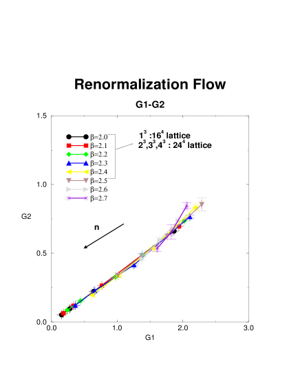
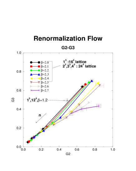
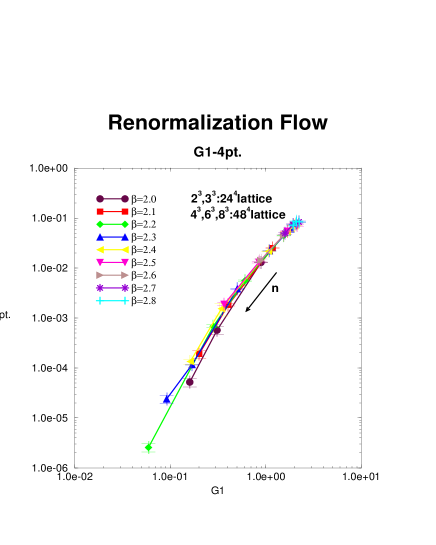
FIG. 2.: The renormalization flow on the projected plane.

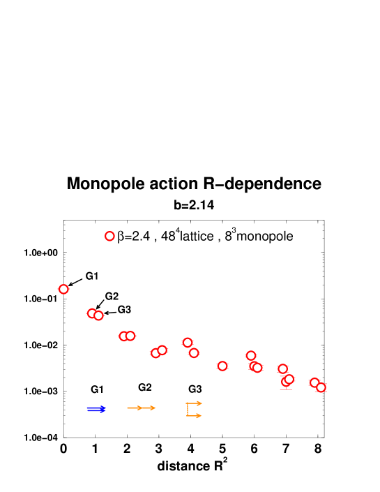
FIG. 3.: The distance dependence of the couplings of quadratic interaction terms at $b=2.14$.

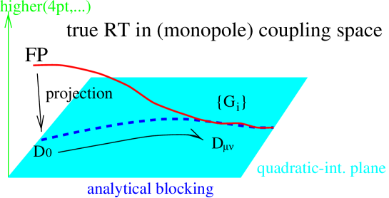
FIG. 4.:

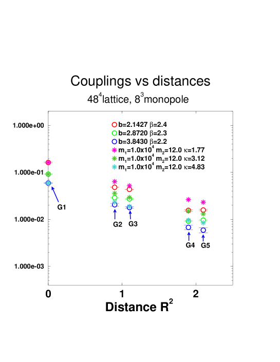
FIG. 5.: The coupling constants with the optimal values $\kappa$, $m_{1}$ and $m_{2}$ for $b=$ 2.1, 2.9 and 3.8 from the comparison with numerical data.

FIG. 6.: The strong coupling expansion of the Wilson loop calculation.

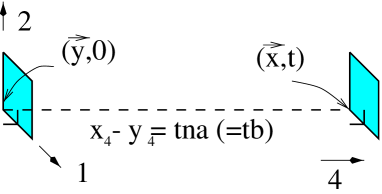
FIG. 7.: The plaquette variable $S_{\alpha\beta}$ for $\langle{\cal O}_{1}\rangle_{m}^{cl}$.

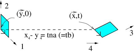
FIG. 8.: The plaquette variable $S_{\alpha\beta}$ for $\langle{\cal O}_{4}\rangle_{m}^{cl}$.

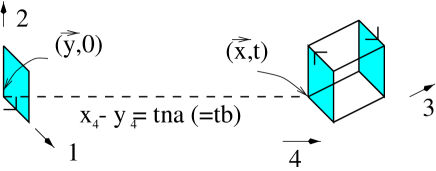
FIG. 9.: The plaquette variable $S_{\alpha\beta}$ for $\langle{\cal O}_{4}\rangle_{m}^{cl}$.

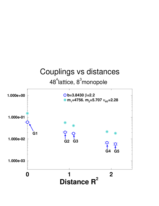
FIG. 10.: The expected coupling constants of RT (star) versus numerical data.

TABLE I.: The optimal values $\kappa$, $m_{1}$ and $m_{2}$ for $b=$ 2.1, 2.9 and 3.8 from the Inverse Monte-Carlo method

$b$	2.1	2.9	3.8
$\kappa$	1.76	3.12	4.83
$m_{1}$	1.0 $\times 10^{4}$	1.0 $\times 10^{4}$	1.0 $\times 10^{4}$
$m_{2}$	12.0	12.0	12.0

TABLE II.: $\sqrt{\sigma_{cl}/\sigma_{phys}}$ for $b=$ 2.1, 2.9 and 3.8.

$b$	2.1	2.9	3.8
$\sqrt{\frac{\sigma_{cl}}{\sigma_{phys}}}$	1.64	1.56	1.45

TABLE III.: The leading quantum correction for $b=$ 2.1, 2.9 and 3.8.

$b$	2.1	2.9	3.8
$\frac{4}{b^{2}}e^{-4\Pi(0)b^{2}}$	$1.26\times 10^{-5}$	$1.40\times 10^{-9}$	$1.65\times 10^{-14}$

TABLE IV.: $M_{0^{++}}/\sqrt{\sigma_{cl}}$ for $b=$ 2.1, 2.9 and 3.8.

$b$	2.1	2.9	3.8
$M_{0^{++}}/\sqrt{\sigma_{cl}}$	5.56	4.18	3.36

TABLE V.: $\sqrt{\sigma_{L}/\sigma_{phys}}$ for $b=$ 2.1, 2.9 and 3.8 from Eq.(31).

$b$	2.1	2.9	3.8
$\sqrt{\frac{\sigma_{L}}{\sigma_{phys}}}$	1.73	1.59	1.39

TABLE VI.: String tensions from non-abelian $(\sigma_{f})$ and monopole $(\sigma_{m})$ Wilson loops.

$\beta$	$\sqrt{\sigma_{f}}a$	$\sqrt{\sigma_{m}}a$
2.20	0.4690(100)	0.4804(52)
2.30	0.3690(30)	0.3589(36)
2.40	0.2660(20)	0.2678(82)
2.50	0.1905(8)	0.1851(32)
2.60	0.1360(40)	0.1346(39)
2.70	0.1015(10)	0.1016(21)

TABLE VII.: The comparison of the three parameters $\bar{\alpha}$ $\bar{\beta}$ $\bar{\gamma}$ between the expected RT and the optimal fit to the numerical data.

$b$	2.1	2.9	3.8
$\bar{\alpha}$	0.565	0.321	0.207
$\bar{\beta}$	6.78	3.85	2.49
$\bar{\gamma}$	$5.65\times 10^{-5}$	$3.21\times 10^{-5}$	$2.07\times 10^{-5}$
$\bar{\alpha}_{RT}$	1.52	0.780	0.435
$\bar{\beta}_{RT}$	6.78	3.85	2.49
$\bar{\gamma}_{RT}$	$4.09\times 10^{-4}$	$1.90\times 10^{-4}$	$9.15\times 10^{-5}$

TABLE VIII.: The quadratic interactions used for the modified Swendsen method.

coupling $\left\{G_{i}\right\}$	distance	type	coupling $\left\{G_{i}\right\}$	distance	type
$G_{1}$	(0,0,0,0)	$k_{\mu}(s)$	$G_{15}$	(2,1,1,0)	$k_{\mu}(s+2\hat{\mu}+\hat{\nu}+\hat{\rho})$
$G_{2}$	(1,0,0,0)	$k_{\mu}(s+\hat{\mu})$	$G_{16}$	(1,2,1,0)	$k_{\mu}(s+\hat{\mu}+2\hat{\nu}+\hat{\rho})$
$G_{3}$	(0,1,0,0)	$k_{\mu}(s+\hat{\nu})$	$G_{17}$	(0,2,1,1)	$k_{\mu}(s+2\hat{\nu}+\hat{\rho}+\hat{\sigma})$
$G_{4}$	(1,1,0,0)	$k_{\mu}(s+\hat{\mu}+\hat{\nu})$	$G_{18}$	(2,1,1,1)	$k_{\mu}(s+2\hat{\mu}+\hat{\nu}+\hat{\rho}+\hat{\sigma})$
$G_{5}$	(0,1,1,0)	$k_{\mu}(s+\hat{\nu}+\hat{\rho})$	$G_{19}$	(1,2,1,1)	$k_{\mu}(s+\hat{\mu}+2\hat{\nu}+\hat{\rho}+\hat{\sigma})$
$G_{6}$	(2,0,0,0)	$k_{\mu}(s+2\hat{\mu})$	$G_{20}$	(2,2,0,0)	$k_{\mu}(s+2\hat{\mu}+2\hat{\nu})$
$G_{7}$	(0,2,0,0)	$k_{\mu}(s+2\hat{\nu})$	$G_{21}$	(0,2,2,0)	$k_{\mu}(s+2\hat{\nu}+2\hat{\rho})$
$G_{8}$	(1,1,1,1)	$k_{\mu}(s+\hat{\mu}+\hat{\nu}+\hat{\rho}+\hat{\sigma})$	$G_{22}$	(3,0,0,0)	$k_{\mu}(s+3\hat{\mu})$
$G_{9}$	(1,1,1,0)	$k_{\mu}(s+\hat{\mu}+\hat{\nu}+\hat{\rho})$	$G_{23}$	(0,3,0,0)	$k_{\mu}(s+3\hat{\nu})$
$G_{10}$	(0,1,1,1)	$k_{\mu}(s+\hat{\nu}+\hat{\rho}+\hat{\sigma})$	$G_{24}$	(2,2,1,0)	$k_{\mu}(s+2\hat{\mu}+2\hat{\nu}+\hat{\rho})$
$G_{11}$	(2,1,0,0)	$k_{\mu}(s+2\hat{\mu}+\hat{\nu})$	$G_{25}$	(1,2,2,0)	$k_{\mu}(s+\hat{\mu}+2\hat{\nu}+2\hat{\rho})$
$G_{12}$	(1,2,0,0)	$k_{\mu}(s+\hat{\mu}+2\hat{\nu})$	$G_{26}$	(0,2,2,1)	$k_{\mu}(s+2\hat{\nu}+2\hat{\rho}+\hat{\sigma})$
$G_{13}$	(0,2,1,0)	$k_{\mu}(s+2\hat{\nu}+\hat{\rho})$	$G_{27}$	(2,1,1,0)	$k_{\rho}(s+2\hat{\mu}+2\hat{\nu}+\hat{\rho})$
$G_{14}$	(2,1,0,0)	$k_{\nu}(s+2\hat{\mu}+\hat{\nu})$

TABLE IX.: The higher order interactions used for the modified Swendsen method.

coupling	distance	type
4-point	(0,0,0,0)	$\quad\quad\sum_{s}\left(\sum_{\mu=-4}^{4}k_{\mu}^{2}(s)\right)^{2}$
6-point	(0,0,0,0)	$\quad\quad\sum_{s}\left(\sum_{\mu=-4}^{4}k_{\mu}^{2}(s)\right)^{3}$

REFERENCES

• [1] K.G. Wilson, Phys. Rev. D14 (1974) 2455.
• [2] G.’t Hooft, Nucl. Phys. B190 (1981) 455.
• [3] A.A. Abrikosov, JETP 32 (1957) 1442.
• [4] A.S. Kronfeld et al., Phys. Lett. 198B (1987) 516; A.S. Kronfeld, G. Schierholz and U.J. Wiese, Nucl. Phys. B293 (1987) 461.
• [5] T. Suzuki and I. Yotsuyanagi, Phys. Rev. D42 (1990) 4257; Nucl. Phys. B (Proc. Suppl.) 20 (1991) 236; S. Hioki et al., Phys. Lett. B272 (1991) 326 and references therein.
• [6] T. Suzuki, Nucl. Phys. B (Proc. Suppl.) 30 (1993) 176;
M. I. Polikarpov, Nucl. Phys. B (Proc. Suppl.) 53 (1997) 134;
G. S. Bali, talk given at 3rd International Conference on Quark Confinement and the Hadron Spectrum (Confinement III), Newport News, VA, June 1998, hep-ph/9809351;
R. W. Haymaker, to be published in Phys. Rept., hep-lat/9809094.
• [7] M.N. Chernodub and M.I. Polikarpov, in ”Confinement, Duality and Nonperturbative Aspects of QCD”, p.387, Ed. by Pierre van Baal, Plenum Press, 1998; hep-th/9710205
• [8] H. Shiba and T. Suzuki, Phys. Lett. B343 (1995) 315, Phys. Lett. B351 (1995) 519 and references therein.
• [9] R.H. Swendsen, Phys. Rev.  Lett. 52 (1984) 1165; Phys. Rev. B30 (1984) 3866,3875.
• [10] J. Smit and A.J. van der Sijs, Nucl. Phys. B355 (1991) 603.
• [11] S. Kato, S. Kitahara, N. Nakamura and T. Suzuki, Nucl. Phys. B520 (1998) 323.
• [12] S. Fujimoto et al, Nucl.Phys.B(Proc.Suppl)73(1999) 533.
• [13] T.A. DeGrand and D. Toussaint, Phys. Rev. D22 (1980) 2478.
• [14] T.L. Ivanenko, A.V. Pochinskii and M.I. Polikarpov, Phys. Lett. B 252 (1990) 631.
• [15] S. Fujimoto et al, A Quantum Perfect Lattice Action for Monopoles and Strings, to be published in Phys. Lett. B, hep-lat/0002006.
• [16] T. Suzuki, Prog.Theor.Phys. 80 (1988) 929; 81 (1989) 752; S. Maedan and T. Suzuki, Prog.Theor.Phys. 80 (1988) 929; S. Maedan $et$ $al$, Prog.Theor.Phys. 84 (1990) 130.
• [17] V.L. Beresinskii, Sov. Phys. JETP 32 (1970) 493.
• [18] J.M. Kosterlitz and D.J. Thouless, J. Phys.,C6 (1973) 1181.
• [19] M.N. Chernodub and M.I. Polikarpov, unpublished.
• [20] I. Montvay and G. Münster, “Quantum Fields on a Latiice” Cambridge University Press.
• [21] M. Teper, hep-th/9812187.
• [22] G.S. Bali et al., Phys. Rev. D54 (1996) 2863.
• [23] J.D. Stack, S.D. Nieman and R.J. Wensley, Phys. Rev. D50 (1994) 3399.
• [24] J. Fingberg, U. Heller and F. Karsch, Nucl. Phys. B392 (1993) 493.
A