Strong Non-Ultralocality of Ginsparg-Wilson
Fermionic Actions

Abstract

It is shown that it is impossible to construct a free theory of fermions on infinite hypercubic Euclidean lattice in even number of dimensions that: (a) is ultralocal, (b) respects the symmetries of hypercubic lattice, (c) chirally nonsymmetric part of its propagator is local, and (d) describes single species of massless Dirac fermions in the continuum limit. This establishes non-ultralocality for arbitrary doubler-free Ginsparg–Wilson fermionic action with hypercubic symmetries (“strong non-ultralocality”), and complements the earlier general result on non-ultralocality of infinitesimal Ginsparg–Wilson–Lüscher symmetry transformations (“weak non-ultralocality”).

1 Introduction

Proper inclusion of chiral dynamics in the framework of lattice-regularized gauge theory has long been one of the main themes in this nonperturbative approach. While there are several useful angles to look at this, the many years of conceptual confusion were primarily caused by the simple fact that lattice theories with naive chiral symmetry can not reproduce the physics of chiral anomaly [1, 2]. At the same time, the departure from naive chiral symmetry to accommodate anomalies typically mutilates other aspects of chiral dynamics.

However, the set of acceptable lattice fermionic actions is rather large, and so it is not implausible that there are actions without naive chiral symmetry, where both the anomalies and the chiral dynamics are accommodated simultaneously. Guided by renormalization group arguments, Ginsparg and Wilson suggested that one should examine lattice Dirac theories in which the chirally nonsymmetric part of the massless propagator is local (coupling decays at least exponentially at long distance) [3]. This is very plausible since the important aspects of chiral dynamics are typically associated with the long distance behavior of the propagator, which is then very mildly affected by the chirally nonsymmetric part of the action. Lattice fermionic actions with this property became known as Ginsparg–Wilson (GW) actions and vectorlike theories defined by them indeed have all the important ingredients of chiral dynamics [3, 4, 5]. More importantly, otherwise acceptable GW actions can be explicitly constructed as demonstrated by the class of operators of Neuberger’s type [6, 7].

Formally appealing feature of the GW approach is that it can be defined through the symmetry principle [8]. The underlying Ginsparg–Wilson–Lüscher (GWL) symmetry operation is rather unconventional and depends on the action itself. It has been proved that if the action is symmetric, then the corresponding infinitesimal GWL transformation can not be ultralocal [9]. In other words, the transformation must rearrange the system in such a way that a given variable is mixed with infinitely many other variables on an unbounded lattice. This is a universal property of GWL symmetry in the presence of hypercubic symmetries (weak non-ultralocality), and it shows that to enforce features of chiral dynamics without naive chiral symmetry requires a delicate cooperation of many degrees of freedom. Aside from conceptual value, weak non-ultralocality has a well defined physical meaning, because it is associated with non-ultralocality of Noether currents corresponding to GWL symmetry.

While understanding general structural properties of GW actions is of prime importance for both conceptual and practical reasons, the progress has been rather slow. This is mainly due to the fact that the defining condition for GW actions is nonlinear, which causes the related problems to be quite nontrivial. An important basic question here is whether GW actions can be ultralocal. This issue has been settled (with negative answer) for commonly studied class of GW actions some time ago [10], and the most general result published so far actually follows from weak non-ultralocality. In particular, it was shown that all GW actions for which chirally nonsymmetric part of the propagator is ultralocal (and nonzero), are non-ultralocal in the presence of hypercubic symmetries [9].

The purpose of this paper is to demonstrate strong non-ultralocality as formulated in Ref. [9], i.e. non-ultralocality of all doubler-free GW fermionic actions respecting the symmetries of the hypercubic lattice. Our proof will follow the strategy developed in Ref. [11], which suggests that it is sufficient to consider two-dimensional momentum restrictions for free theories and investigate the consequences of the GW property at the origin of the Brillouin zone. This leads to an algebraic problem reflecting factorization properties of certain class of polynomials [11]. We will adopt the general formalism of Ref. [9] and develop some basic notions of algebraic geometry that will be needed to keep the presentation self-contained.

2 Lattice Dirac Operators and Ultralocality

Consider an infinite $d$-dimensional hypercubic lattice, where $d$ is an even integer. Let $\psi,\overline{\psi}^{T}$ be the vectors of fermionic variables associated with lattice sites. We will be interested in quadratic expressions (actions) $\overline{\psi}{\bf G}\psi$, defined by the linear operator ${\bf G}$ which acts in the corresponding linear space. The usual gauge–flavor structure of the linear space will be ignored since it will be sufficient for our purposes to consider only operators in unit gauge background. Consequently, the fermionic variables have $2^{d/2}$ spinorial components, and arbitrary matrix ${\bf G}$ can be uniquely expanded in the form

$${\bf G}_{m,n}=\sum_{a=1}^{2^{d}}{\bf G}^{a}_{m,n}\Gamma^{a}$$ (1)

Here $m,n$ label the lattice points, ${\bf G}^{a}$ denotes a matrix with position indices, and $\Gamma^{a}$ is the element of the Clifford basis. Clifford basis is built on gamma–matrices satisfying $\{\gamma_{\mu},\gamma_{\nu}\}=2\delta_{\mu,\nu}{\twelvebb I}$. We will refer to the operators ${\bf G}^{a}$ as Clifford components of ${\bf G}$.

It is useful to define the chirally symmetric (${\bf G}_{C}$) and chirally nonsymmetric (${\bf G}_{N}$) part of arbitrary operator ${\bf G}$, using the $\gamma_{5}$ element of the Clifford algebra, namely

$${\bf G}\;=\;{1\over 2}\gamma_{5}\,\{\gamma_{5},{\bf G}\}+{1\over 2}\gamma_{5}\,[\gamma_{5},{\bf G}]\;\equiv\;{\bf G}_{N}+{\bf G}_{C}$$ (2)

This is a unique decomposition such that $\{{\bf G}_{C},\gamma_{5}\}=0$, and $[{\bf G}_{N},\gamma_{5}]=0$.

Important role in our discussion will be played by the subset ${{\twelvefrak G}^{sl}}$ of operators that are local and respect the symmetries of the hypercubic lattice structure. By locality we mean at least exponential decay of interaction at large distances, and the symmetries of hypercubic lattice include translation invariance and invariance under hypercubic rotations and reflections (hypercubic invariance). The elements ${\bf G}\in{{\twelvefrak G}^{sl}}$ can be equivalently represented by their Fourier image which is diagonal

$$G(p)\;\equiv\;\sum_{a=1}^{2^{d}}G^{a}(p)\Gamma^{a}\qquad\qquad G^{a}(p)\equiv\sum_{n}g_{n}^{a}e^{ip\cdot n}\qquad\qquad g_{n}^{a}\equiv{\bf G}^{a}_{0,n}$$ (3)

Here the functions $G^{a}(p)$ of lattice momenta $p\equiv(p_{1},\ldots,p_{d})$ are complex–valued, periodic with $2\pi$ in all variables, analytic, and further restricted by hypercubic invariance. The concepts discussed in this paragraph are properly defined in Appendix A.

The set of lattice Dirac operators that will be considered can now be defined. We require locality, symmetries of the hypercubic lattice, and correct classical continuum limit.

Definition 1

(Set ${\twelvefrak D}$) Let $D(p)$ be a local symmetric operator (element of ${{\twelvefrak G}^{sl}}$), and let in the vicinity of $p=0$ its Clifford components $D^{a}(p)$ satisfy

$$D^{a}(p)=\cases{ip_{\mu}+O(p^{2}),&if $\Gamma^{a}=\gamma_{\mu}\,$;\cr O(p^{2}),&if $\Gamma^{a}\neq\gamma_{\mu}\,,\forall\mu$\cr}$$ (4)

Collection ${\twelvefrak D}\subset{{\twelvefrak G}^{sl}}$ of such elements $D(p)$ defines the set of lattice Dirac operators.

Note that there are elements both with and without doublers in the set ${\twelvefrak D}$.

Finally, our analysis will focus on the property of ultralocality. This notion reflects the fact that the operator doesn’t couple variables beyond some fixed finite distance:

Definition 2

(Ultralocality) Let ${\cal C}_{N}$ denotes the set of all lattice sites contained in the hypercube of side $2N$, centered at $n=0$, i.e. ${\cal C}_{N}\equiv\{n:|n_{\mu}|\leq N,\,\mu=1,\ldots,d\}$. Operator ${\bf G}$ is said to be be ultralocal if there is a positive integer $N$, so that

$${\bf G}^{a}_{m,n}\;=\;0\,,\qquad\;\forall m,n:(m-n)\not\in{\cal C}_{N}\,,\;\forall a$$

If an ultralocal operator ${\bf G}$ is translation invariant, then Clifford components $G^{a}(p)$ of its Fourier image are functions with finite number of Fourier terms, i.e. $G^{a}(p)\equiv\sum_{n\in{\cal C}_{N}}g_{n}^{a}e^{ip\cdot n}$.

3 Formulation of the Problem

Defining property of GW actions is the locality of chirally nonsymmetric part of the propagator. In other words, ${\bf D}\in{\twelvefrak D}$ is a GW operator if $({\bf D}^{-1})_{N}\in{{\twelvefrak G}^{sl}}$. This is very restrictive since the full massless propagator ${\bf D}^{-1}$ is nonlocal. GWL symmetry thus requires that all this nonlocality is contained in the chirally symmetric part $({\bf D}^{-1})_{C}$. Actions with naive chiral symmetry can be viewed as the limiting case in the set of GW actions as $({\bf D}^{-1})_{N}$ completely vanishes.

In Fourier space the GW property means that all Clifford components of $(D^{-1}(p))_{N}$ are analytic functions on the whole Brillouin zone. This is automatic for arbitrary action with naive chiral symmetry, and can be also rather easily arranged even for ultralocal $D(p)$ with $(D(p))_{N}\neq 0$, [9, 11]. However, in all such known cases $D^{-1}(p)$ has unwanted poles at nonzero momenta, and the theory thus suffers from doubling. This suggests that with only finite number of Fourier components at our disposal, it is perhaps impossible to add to the chirally symmetric operator $D_{C}$ a nonsymmetric part $D_{N}$, that would not interfere with the behavior of the propagator at large distances, and at the same time remove all the unwanted poles originating from $D_{C}$.

We show in the rest of this paper that this is indeed true. More precisely, we will prove the following theorem:

Theorem 1

There is no $D(p)\in{\twelvefrak D}$ such that the following three requirements are satisfied simultaneously:

$(\alpha)$

$D(p)$ is ultralocal.

$(\beta)$

$(D^{-1}(p))_{N}\in{{\twelvefrak G}^{sl}}$.

$(\gamma)$

$(D^{-1}(p))_{C}$ has no poles except when $\,p_{\mu}=0\!\pmod{2\pi},\,\forall\mu$.

4 Auxiliary Statements

We first discuss several auxiliary statements that will be needed.

4.1 Two-Dimensional Restrictions on the Brillouin Zone

The key ingredient that leads to the successful demonstration of Theorem 1 rests upon the realization that one should concentrate on the consequences of analyticity of $(D^{-1})_{N}$ at the origin of the Brillouin zone [11]. This is indeed nontrivial because both $(D^{-1})_{C}$ and $(D^{-1})_{N}$ are functions of all Clifford components $D^{a}$, while at the same time, the former is singular and the latter is analytic at the origin. We will show that to capture the required analytic structure of the functions involved, it is sufficient to consider two-dimensional restrictions on the Brillouin zone. We thus start with the definition of such restrictions in general.

Definition 3

(Restriction $\Sigma^{\rho}$) Let $\rho\in\{1,2,\ldots d\}$ and let $\overline{p}$ denotes the restriction of the momentum variable $p$ defined through

$$\overline{p}_{\mu}\;=\;\cases{q_{\mu},&if $\mu=1,\ldots,\rho$;\cr 0,&if $\mu=\rho+1,\ldots,d$\cr}$$

Map $\Sigma^{\rho}$ that assigns to arbitrary function $f(p)$ of $d$ real variables a function $\overline{f}(q)$ of $\rho$ real variables $q\equiv(q_{1},q_{2},\ldots,q_{\rho})$ through

$$\Sigma^{\rho}\Bigl{[}\,f(p)\,\Bigr{]}\;\equiv\;\overline{f}(q)\;\equiv\;f(\overline{p})$$ (5)

will be referred to as restriction $\Sigma^{\rho}$.

Functions with definite transformation properties under hypercubic group simplify or vanish when restricted through $\Sigma^{\rho}$. The elements of ${{\twelvefrak G}^{sl}}$ simplify accordingly. In particular, for $\Sigma^{2}$ we have the following.

Lemma 1

Let $G(p)\in{{\twelvefrak G}^{sl}}$, and let ${\overline{G}}(q)$ be its restriction under $\Sigma^{2}$ defined through

$${\overline{G}}(q)\;=\;\sum_{a=1}^{2^{d}}{\overline{G}}^{a}(q)\Gamma^{a}\qquad\quad{\overline{G}}^{a}(q)\;=\;\Sigma^{2}\Bigl{[}\,G^{a}(p)\,\Bigr{]}$$

Then ${\overline{G}}(q)$ can be written in the form

$${\overline{G}}(q)\;=\;X(q){\twelvebb I}+\sum_{\mu=1}^{2}Y_{\mu}(q)\gamma_{\mu}+Z(q)\gamma_{1}\gamma_{2}$$ (6)

where $X(q)$,$Y_{\mu}(q)$ and $Z(q)$ are analytic functions of two real variables, periodic with $2\pi$, and satisfying

$$X(q_{1},q_{2})\;=\;X(-q_{1},q_{2})\;=\;X(q_{1},-q_{2})\;=\;X(q_{2},q_{1})$$ (7)

$$Y_{1}(q_{1},q_{2})\;=\;-Y_{1}(-q_{1},q_{2})\;=\;Y_{1}(q_{1},-q_{2})\;=\;Y_{2}(q_{2},q_{1})$$ (8)

$$Z(q_{1},q_{2})\;=\;-Z(-q_{1},q_{2})\;=\;-Z(q_{1},-q_{2})\;=\;-Z(q_{2},q_{1})$$ (9)

Lemma 1 reflects the naive expectation that ${\overline{G}}(q)$ formally looks as an element of ${{\twelvefrak G}^{sl}}$ in two dimensions. The proof is given in Appendix C.

The distinctive property of ultralocal elements of ${{\twelvefrak G}^{sl}}$ is that its Clifford components are polynomials (or are related to polynomials) in suitably chosen variables. In particular, for the restrictions under $\Sigma^{2}$ we have the following result proved in Appendix D.

Lemma 2

Let $G(p)$ be an ultralocal element of ${{\twelvefrak G}^{sl}}$. Then the Clifford components (7-9) of its restriction ${\overline{G}}(q)$ under $\Sigma^{2}$ can be written in the form

$$X(q_{1},q_{2}) = P_{X}(\cos q_{1},\cos q_{2})$$

$$Y_{1}(q_{1},q_{2}) = \sin q_{1}\;P_{Y}(\cos q_{1},\cos q_{2})\;=\;Y_{2}(q_{2},q_{1})$$ (10)

$$Z(q_{1},q_{2}) = \sin q_{1}\sin q_{2}\;P_{Z}(\cos q_{1},\cos q_{2})$$

where $P_{X}$ is a symmetric polynomial in its variables, $P_{Z}$ an antisymmetric polynomial, and $P_{Y}$ a polynomial.

4.2 Useful Algebraic Results

While the GW property is associated with analytic properties of the Fourier transform of the propagator, the proof of Theorem 1 that we give in the next section is essentially algebraic. Lemma 3 below is a well-known result which will turn out to reflect this connection to algebra for ultralocal operators. Lemma 4 and Corollary 1 are rather interesting new results that we will need.

Lemma 3

Let $P(x,y)$, $Q(x,y)$ be two polynomials over the field of complex numbers such that $Q(0,0)=0$, and that the rational function $R(x,y)\equiv P(x,y)/Q(x,y)$ is analytic in some neighborhood of the origin. Then $P$ and $Q$ have common polynomial factor $F$, such that if we write $P=F\tilde{P}$, $Q=F\tilde{Q}$, then $\tilde{Q}(0,0)\neq 0$. The polynomial $F$ of minimal degree is unique up to a constant multiplicative factor, and depends only on $Q$.

Lemma 4

Let $G_{1}(x,y)$, $G_{2}(x,y)$ be polynomials over complex numbers, such that $G_{1}(0,0)\neq 0$, $G_{2}(0,0)\neq 0$. Let further

$$B(x,y)\;\equiv\;x(1-x)\;G_{1}^{2}(x,y)+y(1-y)\;G_{2}^{2}(x,y)$$

If $F(x,y)P(x,y)\,=\,B(x,y)$ is arbitrary polynomial factorization such that

$$F(0,0)=0\qquad\qquad\quad P(0,0)\neq 0$$

then $F(x,y)$ must have at least one additional zero on the set ${\cal Z}_{0}\equiv\{\,(x,y):\,x,y\in\{0,1\}\,\}$.

Corollary 1

Let $G_{1}(x^{2},y^{2})$, $G_{2}(x^{2},y^{2})$ be polynomials over complex numbers, such that $G_{1}(0,0)\neq 0$, $G_{2}(0,0)\neq 0$. Let further

$$B(x^{2},y^{2})\;\equiv\;x^{2}(1-x^{2})\;G_{1}^{2}(x^{2},y^{2})+y^{2}(1-y^{2})\;G_{2}^{2}(x^{2},y^{2})$$

If $F(x,y)P(x,y)\,=\,B(x^{2},y^{2})$ is arbitrary polynomial factorization such that

$$F(0,0)=0\qquad\qquad\quad P(0,0)\neq 0$$

then $F(x,y)$ must have at least two additional zeroes on the set ${\cal Z}_{1}\equiv\{\,(x,y):\,x,y\in\{-1,0,1\}\,\}$.

We prove these auxiliary statements in the subsections below. It turns out that it is quite useful and natural for our purposes to use the established language of algebraic geometry. To make this paper sufficiently self-contained, we will first summarize some basic notions and state some standard results that will be relevant for our purposes.

4.2.1 Preliminaries from Algebraic Geometry

We will be repeatedly concerned here with polynomials over the field of complex numbers ${\twelvebb C}$. Let us thus denote the set of such polynomials in indeterminates $x_{1},x_{2},\ldots,x_{n}$ as ${\twelvebb C}\,[x_{1},x_{2},\ldots,x_{n}]$. The degree of arbitrary polynomial $P$ will be denoted as $\mathop{\rm deg}P$. Also, if some expression $Q(x_{1},\ldots,x_{n},y_{1},\ldots,y_{m})$ can be viewed as a power series in variables $x_{1},\ldots,x_{n}$, then $\mathop{\rm ord}_{x_{1},\ldots,x_{n}}(Q)$ will denote the minimal degree of monomials appearing in such series. This obviously applies also if $Q$ is a polynomial. For example, we will work with the power series like $\pi(t)\equiv\sum_{i=0}^{\infty}p_{i}t^{i}$, in which case $\mathop{\rm ord}_{t}(\pi(t))$ is the least $i$ such that $p_{i}\neq 0$.

Definition 4

(Affine Algebraic Curve) Let $P\in{\twelvebb C}\,[x,y]$ and $\mathop{\rm deg}P>0$. The set of points in the complex affine plane $\Gamma_{P}\,\equiv\,\{\,(x,y)\,:\,P(x,y)=0\,\}$ defines an affine algebraic curve.

An algebraic curve is thus a geometric figure defined by the locus of zeroes of a polynomial. Arbitrary neighborhood of any point on the curve contains infinitely many other points belonging to the curve, and there are no isolated points. If $\Gamma$ is an algebraic curve and there exists an irreducible polynomial $P$ such that $\Gamma=\Gamma_{P}$, then $\Gamma$ is called an irreducible algebraic curve. If $P(x,y)$ is reducible and $P(x,y)=\prod_{i=1}^{N}P_{i}^{n_{i}}(x,y)$ is a factorization into irreducible factors, then obviously $\Gamma_{P}\,=\,\Gamma_{P_{1}}\cup\Gamma_{P_{2}}\cup\ldots\Gamma_{P_{N}}$, and the irreducible curves $\Gamma_{P_{i}}$ are referred to as the components of $\Gamma_{P}$.

Introducing the geometrical viewpoint into algebraic problem frequently turns out to be quite useful. Note, for example, that the content of Lemma 4 can be interpreted in the following way. To every polynomial $B(x,y)$ constructed as prescribed we can assign the curve $\Gamma_{B}$, and always ${\cal Z}_{0}\subset\Gamma_{B}$. Similarly, to any factor $F(x,y)$ such that $F(0,0)=0$, we can assign a curve $\Gamma_{F}\subset\Gamma_{B}$, running through the origin. The claim is that every $\Gamma_{F}$ has to run through one additional point of ${\cal Z}_{0}$. To demonstrate this result, we will need some basic tools from the theory of intersections of algebraic curves which, in turn, is more elegantly discussed in the projective plane rather than in the affine plane.

A. Projective Curves

Two parallel lines in the affine plane do not have any points in common. However, it is intuitively quite acceptable to say that they meet at the “point at infinity”. To handle such “intersections” easily, it is useful to think about algebraic curves in the projective plane.

Definition 5

(Projective Plane) Consider the set $S={{\twelvebb C}}^{3}-\{(0,0,0)\}$ and define two points ${\mathbf{a}},{\mathbf{b}}\in S$ to be equivalent iff ${\mathbf{a}}=\lambda{\mathbf{b}}$ for some $\lambda\in{\twelvebb C}$. The set of equivalence classes of $S$ under this equivalence relation is called the projective plane.

A point in the projective plane has thus infinitely many triples of numbers (not simultaneously zero) associated with it. Any one of these fully represents the point and is referred to as a triple of homogeneous coordinates for that point. The coordinates $\{x,y,z\}$ on ${\twelvebb C}^{3}$ are thus used to define the sets of homogeneous coordinates for the points of projective plane. The subset of projective plane consisting of points represented by homogeneous coordinates with $z\neq 0$ is isomorphic to the affine plane under the map

$$\phi\;:\quad(\,x,y,z\,)\quad\longrightarrow\quad(\,{x\over z},{y\over z}\,)$$ (11)

Similarly, the subsets of projective plane with $x\neq 0$ and $y\neq 0$ are isomorphic to the affine plane under analogously defined maps. However, in our discussion we will use the convention fixed by eq. (11).

To understand why projective plane is useful for dealing with points at infinity, consider an arbitrary line in the affine plane. This is specified by linear equation $ax+by+c=0$, where $a,b$ are not simultaneously zero. For definiteness, assume that $b\neq 0$ so that the line can be parametrized through $x$ as $(\,x,-xa/b-c/b\,)$. In view of map $\phi$, this corresponds in the projective plane to the set of points represented by homogeneous coordinates $(\,x,-xa/b-c/b,1\,)$. Concentrating on the part of the line when $|x|$ is very large, we can multiply by $b/x$ and use the homogeneous coordinates $(\,b,-a-c/x,b/x\,)$ instead. Considering now the limiting case $|x|\,\rightarrow\,\infty$, it is natural to associate the point at infinity of the affine plane corresponding to the above line with the point in the projective plane with homogeneous coordinates $(\,b,-a,0\,)$. Notice that this point is not part of the isomorphism realized through (11) and there are no infinities associated with this point in the projective plane. Thus, roughly speaking, the projective plane is an affine plane together with its points at infinity.

Definition 6

(Projective Algebraic Curve) Let $P\in{\twelvebb C}\,[x,y,z]$ be homogeneous of nonzero degree. The set of points in the complex projective plane represented by homogeneous coordinates from the set $\Gamma_{P}\,\equiv\,\{\,(x,y,z)\,:\,P(x,y,z)=0\,\}$ defines a projective algebraic curve.

We deal with homogeneous polynomials in projective plane because they simultaneously vanish for all homogeneous coordinates representing the same point of the projective plane. The concepts of irreducibility and component are defined analogously to the affine case, i.e. through irreducibility of the defining homogeneous polynomial.

There is a natural one to one correspondence between affine curves and projective curves that do not have $z=0$ (line at infinity) as a component. To see that, it is useful to consider the map $\Phi$ which assigns to arbitrary $P\in{\twelvebb C}\,[x,y]$ of degree $m$, the homogeneous polynomial $P^{*}\in{\twelvebb C}\,[x,y,z]$ of the same degree through

$$\Phi\;:\quad P(x,y)\quad\longrightarrow\quad P^{*}(x,y,z)\,\equiv\,z^{m}\,P(\,{x\over z},{y\over z}\,)$$ (12)

The image $P^{*}$ of $P$ under $\Phi$ is usually referred to as the canonical homogenization of $P$. The following obvious theorem holds (see e.g. Ref. [14])

Theorem 2

$\Phi$ is a bijective map (one to one and onto) between ${\twelvebb C}\,[x,y]$ and the set ${\cal H}\subset{\twelvebb C}\,[x,y,z]$ of homogeneous polynomials not divisible by $z$. The corresponding inverse map is given by $P^{*}(x,y,z)\,\rightarrow\,P(x,y)\,\equiv\,P^{*}(x,y,1)$. Polynomial $P(x,y)$ is irreducible if and only if its image $P^{*}(x,y,z)$ is irreducible.

In this way bijection $\Phi$ also defines the correspondence between affine curve $\Gamma_{P}$ and projective curve $\Gamma_{P^{*}}$, where the points are associated through map $\phi$ of eq. (11). For any point $(x,y)$ of the affine curve $\Gamma_{P}$ there is a corresponding point on projective curve $\Gamma_{P^{*}}$, represented for example by $(x,y,1)$. Conversely, for arbitrary point of the projective curve $\Gamma_{P^{*}}$ with homogeneous coordinates $(x,y,z),\;z\neq 0$, there is a corresponding point $(x/z,y/z)$ on $\Gamma_{P}$. The points on $\Gamma_{P^{*}}$ with homogeneous coordinates $(x,y,0)$ do not have the corresponding points in the finite affine plane and they are the points at infinity of $\Gamma_{P}$. In this sense, the projective curve $\Gamma_{P^{*}}$ is frequently referred to as the projective closure of $\Gamma_{P}$. Conversely, $\Gamma_{P}$ is an affine representative of $\Gamma_{P^{*}}$.

B. Intersections of Curves

Our discussion of curve intersections will focus on understanding the most basic result here, namely the Bezout’s Theorem. The logic and formalism of our approach will be almost exclusively guided by its utility in the proof of Lemma 4.

We start with the notion of intersection multiplicity, which is a positive integer assigned to any point where two algebraic curves meet. The corresponding definition is motivated by the concept of multiplicity for the root of a polynomial. Let us first consider a simple example in the affine plane. The curve $\Gamma_{P}$ cut out by the polynomial $P(x,y)=y-F(x)$ and the curve $\Gamma_{L}$ with $L(x,y)=y$ (line) meet at some point $(\lambda,0)$. In this case one can easily define the intersection multiplicity at that point as the multiplicity of $\lambda$ as a root of $F$. Knowledge of intersection multiplicity assigned this way clearly adds a useful geometrical detail on how the two curves actually meet. It is instructive to think of this definition of intersection multiplicity also in a different way. Consider the parametrization $t\longrightarrow(t+\lambda,0)$ of the line $\Gamma_{L}$. Since $t=0$ corresponds to the point $(\lambda,0)$, such parametrization is usually referred to as parametrization “at the point” $(\lambda,0)$. Upon insertion in $P(x,y)$ we get $P(\lambda+t,0)=-F(\lambda+t)$, and we can conclude that the intersection multiplicity of $\Gamma_{P}$ and $\Gamma_{L}$ at the point $(\lambda,0)$ is given by $\mathop{\rm ord}_{t}(F(\lambda+t))\,=\,\mathop{\rm ord}_{t}(P(\lambda+t,0))$. We have just used an elementary fact that if $F(x)$ is a polynomial in ${\twelvebb C}[x]$, then the multiplicity of $\lambda$ as a root of $F$ is given by $\mathop{\rm ord}_{t}(F(t+\lambda))$.

Our aim is to generalize the above method for arbitrary curves. To do this, it is first necessary to put the concept of parametrization at a point of a curve on a firm footing. The following fundamental statement holds [15]

Theorem 3

Let $\Gamma_{P}$ be arbitrary projective algebraic curve, and let $(x_{0},y_{0},z_{0})$ be arbitrary point of this curve. There exists a finite set of triples of functions $(\mu_{j}(t),\nu_{j}(t),\xi_{j}(t))$, analytic in the neighborhood of $t=0$, such that

(1) $(\mu_{j}(0),\nu_{j}(0),\xi_{j}(0))\,=\,(x_{0},y_{0},z_{0})\,,\;\forall j$

(2) $P(\mu_{j}(t),\nu_{j}(t),\xi_{j}(t))\,=\,0\,,\;\forall j$

(3) For every point $(x,y,z)\neq(x_{0},y_{0},z_{0})$ of $\Gamma_{P}$ in a suitable neighborhood of $(x_{0},y_{0},z_{0})$, there is exactly one $j$ and a unique value of $t$ such that $(\mu_{j}(t),\nu_{j}(t),\xi_{j}(t))=(x,y,z)$.

It should be emphasized that the set of triples $(\mu_{j}(t),\nu_{j}(t),\xi_{j}(t))$ of Theorem 3 is not unique. In particular, we can perform an analytic change of variables $t=\alpha_{1}\tau+\alpha_{2}\tau^{2}+\ldots\;,\,\alpha_{1}\neq 0$, to obtain an equally valid parametric representation (in $\tau$) satisfying conditions ${\mathit{(}1-3)}$. For fixed $j$, the equivalence class of such representations is usually referred to as a branch. The point $(\mu_{j}(0),\nu_{j}(0),\xi_{j}(0))$ is said to be the center of the branch, and the branch is said to be centered at that point. Completely analogous considerations hold for affine curves. As a simple example of multiple branches centered at a point, we can consider the curve defined by $P(x,y)=y^{2}-x^{2}-x^{3}$, which has two branches at the origin given by $t\longrightarrow(\,t,t(1+t)^{1/2}\,)$ and $t\longrightarrow(\,t,-t(1+t)^{1/2}\,)$.

Definition 7

(Intersection Multiplicity) Let ${\mathbf{a}}\equiv(x_{0},y_{0},z_{0})$ be the intersection point of projective algebraic curves $\Gamma_{P}$ and $\Gamma_{Q}$. Let further $\Gamma_{P}$ have $N$ branches $\gamma_{j}\equiv(\mu_{j}(t),\nu_{j}(t),\xi_{j}(t))$ centered at ${\mathbf{a}}$. The intersection multiplicity of $\Gamma_{P}$ and $\Gamma_{Q}$ at point ${\mathbf{a}}$ is defined as

$$i(\Gamma_{P},\Gamma_{Q},{\mathbf{a}})\,\equiv\,\sum_{j=1}^{N}i(\gamma_{j},\Gamma_{Q},{\mathbf{a}})\,\equiv\,\sum_{j=1}^{N}{\mathop{\rm ord}}_{t}\Bigl{(}Q(\mu_{j}(t),\nu_{j}(t),\xi_{j}(t))\Bigr{)}$$

where $i(\gamma_{j},\Gamma_{Q},{\mathbf{a}})$ is the intersection multiplicity of $\gamma_{j}$ and $\Gamma_{Q}$ at point ${\mathbf{a}}$.

It can be shown that the above definition of $i(\Gamma_{P},\Gamma_{Q},{\mathbf{a}})$ is symmetric in $\Gamma_{P}$, $\Gamma_{Q}$, and that it is not dependent on the specific choice of parametrization from the corresponding equivalence classes defining the branches.

We are now finally in the position to state the fundamental theorem about intersections of curves in the projective plane [14].

Theorem 4

(Bezout’s Theorem) Let $\Gamma_{P}$ and $\Gamma_{Q}$ be two projective algebraic curves without a common component. The total number of their intersections counted with multiplicities is given by $i(\Gamma_{P},\Gamma_{Q})\,=\,\mathop{\rm deg}P\mathop{\rm deg}Q$.

4.2.2 Proof of Lemma 3

Proof. Consider the factorization of $Q$ into irreducible factors, and splitting these factors in two groups. In particular, we label the factors that vanish at the origin as $F_{i}$, and the factors that do not vanish at the origin as $\tilde{Q}_{i}$. Using this, define $F(x,y)\equiv\prod_{i=1}^{n}F_{i}(x,y)$ and $\tilde{Q}(x,y)\equiv\prod_{i=1}^{m}\tilde{Q}_{i}(x,y)$. Note that while there is always at least one $F_{i}$, there doesn’t necessarily have to be any $\tilde{Q}_{i}$. In that case we define $\tilde{Q}(x,y)\equiv 1$. We thus always have $Q=F\tilde{Q}$, with $F(0,0)=0$, and $\tilde{Q}(0,0)\neq 0$.

Let us look at an arbitrary but fixed $F_{i}$, defining an irreducible affine complex algebraic curve $\Gamma_{F_{i}}$, running through the origin. Consider an arbitrary (complex) neighborhood of the origin, in which $R(x,y)$ is analytic. Any such neighborhood contains infinitely many points of $\Gamma_{F_{i}}$. These points represent locations of potential singularities of $R(x,y)$, and thus must be canceled by zeroes of $P(x,y)$. However, by Bezout’s theorem, any two algebraic curves without common component have only finite number of points in common so this is only possible if $\Gamma_{F_{i}}$ is the component of $\Gamma_{P}$. Consequently, $F_{i}$ must be an irreducible factor of $P$.

By the above argument, $F$ is the desired common factor of $P$ and $Q$. From the unique factorization theorem it follows that $F$ is the only factor (up to a multiplicative constant) of minimal degree. Also, its definition only depends on $Q$ as claimed.   

4.2.3 Proof of Lemma 4

We will use the formalism described in section 4.2.1 to view Lemma 4 as the problem of algebraic geometry. In particular, we will assign to the polynomials $G_{1}(x,y)$, $G_{2}(x,y)$ and $B(x,y)$ their canonical homogenizations defined by the map $\Phi$ of equation (12). In view of Theorem 2 we can then reformulate the problem equivalently in projective terms as follows.

Proposition 1

Let $G_{1}(x,y,z),G_{2}(x,y,z)\in{\twelvebb C}\,[x,y,z]$ be homogeneous polynomials, such that $G_{1}(0,0,1)\neq 0$, $G_{2}(0,0,1)\neq 0$. Let further

$$B(x,y,z)\;\equiv\;x(z-x)\;G_{1}^{2}(x,y,z)+y(z-y)\;G_{2}^{2}(x,y,z)$$

If $F(x,y,z)P(x,y,z)\,=\,B(x,y,z)$ is arbitrary polynomial factorization such that

$$F(0,0,1)=0\qquad\qquad\quad P(0,0,1)\neq 0$$

then the projective algebraic curve $\Gamma_{F}$ passing through $(0,0,1)$ must pass through at least one additional point from the set $\tilde{{\cal Z}}_{0}\equiv\{\,(x,y,1):\,x,y\in\{0,1\}\,\}$.

Proof. For convenience, let us denote $F_{1}(x,y,z)=x(z-x)$ and $F_{2}(x,y,z)=y(z-y)$. We will concentrate on the intersections of $\Gamma_{F}$ with $\Gamma_{F_{1}}$. It is sufficient to consider factors $F$ that do not have common polynomial factor with $F_{1}$. Indeed, $x$ can not be a factor of $B$, and hence it can not be a factor of $F$. On the other hand, $z-x$ can be a factor of $F$ but if it is, than the claim of the proposition is obviously true.

(I) Since $F_{1}$ and $F$ are mutually coprime, it follows from Bezout’s theorem that the total number of their intersections $i(\Gamma_{F},\Gamma_{F_{1}})$ counted with multiplicities is even.

(II) Let ${\mathbf{a}}$ be the intersection point of $\Gamma_{F}$ and $\Gamma_{F_{1}}$ such that ${\mathbf{a}}\notin\Gamma_{F_{2}}$. Then the intersection multiplicity $i(\Gamma_{F},\Gamma_{F_{1}},{\mathbf{a}})$ is even. Indeed, let $\gamma\equiv(\mu(t),\nu(t),\xi(t))$ be arbitrary branch of $\Gamma_{F}$ centered at ${\mathbf{a}}$. Then $B(\mu(t),\nu(t),\xi(t))=0$, or equivalently

$$F_{1}F_{2}G_{1}^{2}\,=\,-F_{2}^{2}G_{2}^{2}\qquad\mbox{\rm for}\qquad(x,y,z)\longrightarrow(\mu(t),\nu(t),\xi(t))$$ (13)

Because of the squares, we can conclude that upon the substitution, $\mathop{\rm ord}_{t}(F_{1}\,F_{2})$ is even. At the same time, since ${\mathbf{a}}\notin\Gamma_{F_{2}}$, we have $F_{2}(\mu(0),\nu(0),\xi(0))\neq 0$, and thus $\mathop{\rm ord}_{t}(F_{2})=0$. But $\mathop{\rm ord}_{t}(F_{1}\,F_{2})=\mathop{\rm ord}_{t}(F_{1})+\mathop{\rm ord}_{t}(F_{2})$, and so $\mathop{\rm ord}_{t}(F_{1})=i(\gamma,\Gamma_{F_{1}},{\mathbf{a}})$ is a positive even integer. Since this is true for all branches $\gamma$ of $\Gamma_{F}$ centered at ${\mathbf{a}}$, we can conclude that $i(\Gamma_{F},\Gamma_{F_{1}},{\mathbf{a}})$ is even as claimed.

(III) If ${\mathbf{a}}=(0,0,1)$, then $i(\Gamma_{F},\Gamma_{F_{1}},{\mathbf{a}})=1$. Indeed, $\Gamma_{F_{1}}$ has a single branch centered at ${\mathbf{a}}$, namely the line that can be parametrized as $\lambda=(0,t,1)$. Since $P(0,0,1)\neq 0$ and $G_{2}(0,0,1)\neq 0$ we have

$$i(\Gamma_{F},\Gamma_{F_{1}},{\mathbf{a}}_{1})\,=\,{\mathop{\rm ord}}_{t}\Bigl{(}F(0,t,1)\Bigr{)}\,=\,{\mathop{\rm ord}}_{t}\Bigl{(}F(0,t,1)P(0,t,1)\Bigr{)}\,=\,{\mathop{\rm ord}}_{t}\Bigl{(}t(1-t)G_{2}^{2}(0,t,1)\Bigr{)}\,=\,1$$

For (I-III) to be satisfied simultaneously, $\Gamma_{F}$ and $\Gamma_{F_{1}}$ must necessarily intersect at one additional point from the set of points where $\Gamma_{F_{1}}$ and $\Gamma_{F_{2}}$ meet. However, this set is precisely represented by the set of homogeneous coordinates from $\tilde{{\cal Z}}_{0}$. Consequently, $\Gamma_{F}$ has to pass through one additional point from $\tilde{{\cal Z}}_{0}$ as claimed.   

4.2.4 Proof of Corollary 1

Proof. Let us consider an arbitrary but fixed polynomial $B(x^{2},y^{2})$ of the prescribed form, and the set of all factorizations $B(x^{2},y^{2})=F(x,y)P(x,y)$ with required properties. It will be sufficient to prove the statement for the case when $F(x,y)$ does not contain any nontrivial polynomial factor with nonzero constant term. Indeed, if $F(x,y)$ has such a factor $P_{1}(x,y)$, then redefining $F(x,y)\rightarrow F(x,y)/P_{1}(x,y)$, $P(x,y)\rightarrow P(x,y)P_{1}(x,y)$ can only make the set of zeroes for new $F(x,y)$ smaller. As a consequence of the unique factorization theorem, the factors $F$, $P$ are unique up to a trivial rescaling by complex number if this additional condition is imposed.

Assuming the above, consider the transformation $x\rightarrow-x$, which does not change $B(x^{2},y^{2})$. Since all possible nontrivial irreducible factors $F_{i}(x,y)$ of $F(x,y)$ satisfy $F_{i}(0,0)=0$, while all irreducible factors $P_{i}(x,y)$ of $P(x,y)$ have $P_{i}(0,0)\neq 0$, it follows from the unique factorization theorem that $F(x,y)\rightarrow F(x,y)$ and $P(x,y)\rightarrow P(x,y)$ under the above reflection. The same is true under $y\rightarrow-y$ and, as a result, $F=F(x^{2},y^{2})$, $P=P(x^{2},y^{2})$. This implies that we can change the variables $x^{2}\rightarrow x$, $y^{2}\rightarrow y$ in the whole problem. In new variables, we have

$$B(x,y)\;\equiv\;x(1-x)\,G_{1}^{2}(x,y)+y(1-y)\,G_{2}^{2}(x,y)\;=\;F(x,y)\,P(x,y)$$

with properties at the origin preserved. However, according to Lemma 4, $F(x,y)$ must have an additional zero on the set ${\cal Z}_{0}\equiv\{\,(x,y):\,x,y\in\{0,1\}\,\}$. Consequently, $F(x^{2},y^{2})$ must vanish for at least two additional points from the set ${\cal Z}_{1}\equiv\{\,(x,y):\,x,y\in\{-1,0,1\}\,\}$ which completes the proof.   

5 Proof of Strong Non-Ultralocality (Theorem 1)

We now use the formalism of Sec. 2 and auxiliary statements of Sec. 4 to prove “strong non-ultralocality” of GW actions (Theorem 1).

Proof. We will proceed by contradiction, and thus first assume that there actually exists an element $D(p)\in{\twelvefrak D}$ such that the requirements $(\alpha-\gamma)$ are satisfied. To this $D(p)$ we will assign its restriction ${\overline{D}}(q)$ under $\Sigma^{2}$ which, according to Lemma 1, has the form $(\,q\equiv(q_{1},q_{2})\,)$

$${\overline{D}}(q)\;=\;\overline{A}(q)\,{\twelvebb I}\,+\,i\sum_{\mu=1}^{2}\overline{B}_{\mu}(q)\,\gamma_{\mu}\,+\,\overline{C}(q)\,\gamma_{1}\gamma_{2}$$ (14)

with the corresponding propagator being

$${\overline{D}}^{-1}\;=\;{{\;\overline{A}\;}\over{\;\overline{Q}\;}}\,{\twelvebb I}\,-\,i\sum_{\mu=1}^{2}{{\,\overline{B}_{\mu}\,}\over{\;\overline{Q}\;}}\,\gamma_{\mu}\,-\,{{\;\overline{C}\;}\over{\;\overline{Q}\;}}\,\gamma_{1}\gamma_{2}\qquad\quad\overline{Q}\;\equiv\;\overline{A}^{2}+\overline{B}_{\mu}\overline{B}_{\mu}+\overline{C}^{2}$$ (15)

Note that according to conditions $(\beta)$ and $(\gamma)$, no Clifford component of ${\overline{D}}^{-1}$ has a pole away from the origin of the Brillouin zone. Consequently, the function

$$\Bigl{(}{{\;\overline{A}\;}\over{\;\overline{Q}\;}}\Bigr{)}^{2}\,+\,\Bigl{(}{{\,\overline{B}_{\mu}\,}\over{\;\overline{Q}\;}}\Bigr{)}\Bigl{(}{{\,\overline{B}_{\mu}\,}\over{\;\overline{Q}\;}}\Bigr{)}\,+\,\Bigl{(}{{\;\overline{C}\;}\over{\;\overline{Q}\;}}\Bigr{)}^{2}\;=\;{{\;1\;}\over{\;\overline{Q}\;}}$$ (16)

has also no poles away from the origin.

Since ${\overline{D}}(q)$ is ultralocal, we can use Lemma 2, to conclude that its Clifford components have the following structure

$$\overline{A}(q_{1},q_{2}) = P_{\overline{A}}(\cos q_{1},\cos q_{2})$$

$$\overline{B}_{1}(q_{1},q_{2}) = \sin q_{1}\,P_{\overline{B}}(\cos q_{1},\cos q_{2})\;=\;\overline{B}_{2}(q_{2},q_{1})$$ (17)

$$\overline{C}(q_{1},q_{2}) = \sin q_{1}\sin q_{2}\,P_{\overline{C}}(\cos q_{1},\cos q_{2})$$

where $P_{\overline{A}}$ is a symmetric polynomial, $P_{\overline{C}}$ an antisymmetric polynomial, and $P_{\overline{B}}$ a polynomial without definite symmetry properties. The classical continuum limit (4) requires that $P_{\overline{A}}(1,1)=0$, $P_{\overline{B}}(1,1)=1$, and also $P_{\overline{C}}(1,1)=0$ by virtue of its antisymmetry.

The GW property $(\beta)$ demands that the Clifford components of chirally nonsymmetric part of the propagator ($\overline{A}/\overline{Q}$ and $\overline{C}/\overline{Q}$) are analytic in some complex region containing the (real) Brillouin zone. We will concentrate on the consequences of analyticity in the vicinity of the origin. To this end, it is convenient to introduce a change of variables such as

$$x\;=\;\sin\,{q_{1}\over 2}\qquad\qquad y\;=\;\sin\,{q_{2}\over 2}$$ (18)

which is invertible in the vicinity of the origin, maps the real region $[-\pi,\pi]\times[-\pi,\pi]$ onto the square $[-1,1]\times[-1,1]$, and preserves analyticity in new variables except possibly on the boundary. Using (5), we have

$$\overline{A}(q_{1},q_{2}) = A(x^{2},y^{2})$$

$$\overline{B}_{1}(q_{1},q_{2}) = x\,\sqrt{1-x^{2}}\,G(x^{2},y^{2})\;=\;\overline{B}_{2}(q_{2},q_{1})$$ (19)

$$\overline{C}(q_{1},q_{2}) = \sqrt{\mathstrut 1-x^{2}}\,\sqrt{\mathstrut 1-y^{2}}\,xy\,C(x^{2},y^{2})$$

where $A$ is a symmetric polynomial such that $A(0,0)=0$, $C$ is an antisymmetric polynomial, and $G$ is a polynomial such that $G(0,0)=2$. It is also convenient to introduce symmetric polynomials

$$B(x^{2},y^{2})\;\equiv\;x^{2}(1-x^{2})\,G^{2}(x^{2},y^{2})\,+\,y^{2}(1-y^{2})\,G^{2}(y^{2},x^{2})$$ (20)

$$Q(x^{2},y^{2})\;\equiv\;A^{2}(x^{2},y^{2})\,+\,B(x^{2},y^{2})\,+\,x^{2}y^{2}(1-x^{2})(1-y^{2})\,C^{2}(x^{2},y^{2})$$ (21)

corresponding to $\overline{B}_{\mu}\overline{B}_{\mu}$, and $\overline{Q}$ respectively. With this notation, the GW property $(\beta)$ implies that the functions

$$R_{1}(x^{2},y^{2})\,\equiv\,{A(x^{2},y^{2})\over Q(x^{2},y^{2})}\qquad\quad R_{2}(x,y)\,\equiv\,\sqrt{\mathstrut 1-x^{2}}\;\sqrt{\mathstrut 1-y^{2}}\;xy\;{{C(x^{2},y^{2})}\over{Q(x^{2},y^{2})}}$$

are analytic in the vicinity of the origin.

Let us first consider $R_{1}$ which is a rational function whose denominator vanishes at the origin. Consequently, according to Lemma 3, the polynomials $A$ and $Q$ have a common polynomial factor $F(x,y)$ with zero at the origin, so that the possible singularity is removed. Let us fix $F$ to be of minimal degree, and thus unique up to a constant multiplicative factor. Next, consider $R_{2}$. Since $\sqrt{1-x^{2}}$ and $\sqrt{1-y^{2}}$ are analytic and nonzero near the origin, the rational function $xyC/Q$ is also analytic and, moreover, the same denominator $Q$ is involved as in $R_{1}$. Consequently, the polynomial $F$ divides $xy\,C$. In summary, we thus have that $F$ divides $A$,$\;xyC$ and $Q$. Hence, from the form (21) of $Q$ it follows that $F$ also divides $B$.

According to Corollary 1, an intriguing property of any polynomial $B(x^{2},y^{2})$ of the form (20) is that if it is divisible by polynomial $F(x,y)$ vanishing at the origin, then $F$ has at least two additional zeroes on the set of points ${\cal Z}_{1}=\{\,(x,y):\,x,y\in\{-1,0,1\}\,\}$. Since $F$ divides $Q$, it follows that $Q$ also has these zeroes on ${\cal Z}_{1}$. Returning back to momentum variables, we thus came to the conclusion that in addition to the origin of the Brillouin zone, the function $\overline{Q}(q)$ of equation (15) has at least two additional zeroes on the set $\tilde{\cal Z}_{1}=\{\,(q_{1},q_{2}):\,q_{1},q_{2}\in\{-\pi,0,\pi\}\,\}$. However, this contradicts the conclusion of (16) that $1/\overline{Q}$ has no poles away from the origin of the Brillouin zone. That completes the proof.   

We have thus demonstrated that every ultralocal GW action with hypercubic symmetries has a doubler. The argument given above can be refined using the statement of Proposition 3, formulated and proved in Appendix E. This implies that there is always a doubler at the corner $(\pi,\pi)$ of the restricted Brillouin zone.

6 Conclusions

As a result of several breakthroughs in the last decade, lattice field theory appears to have finally reached the stage when it can deal with all the important symmetries relevant in particle physics. In particular, it is now conceptually quite clear how to formulate at least vectorlike lattice models simultaneously possessing the lattice counterparts of gauge symmetry (Wilson gauge symmetry), Poincaré symmetry (symmetries of hypercubic lattice) and chiral symmetry (GWL symmetry), so that the continuum limit with desired field-theoretic properties can be taken comfortably. The path of developments leading to this point essentially coincides with the attempts to better understand lattice fermionic actions. Fig. 1 is a graphical representation of the basic knowledge that we now have [11], including the result on strong non-ultralocality demonstrated here.

The base set $A$ in Fig. 1 represents all actions quadratic in fermionic variables, that have “easy symmetries” (gauge and hypercubic symmetries), and proper classical continuum limit. In other words, it is the set of fermionic actions described by lattice Dirac kernels that are covariant under symmetry transformations of hypercubic lattice, gauge covariant, and with classical limit corresponding to continuum Dirac operator. The base set $A$ is split into three parts $A=A^{U}\cup A^{L}\cup A^{N}$, representing the actions that are ultralocal, local but not ultralocal, and nonlocal respectively. Highlighted is also the subset of actions without doubling of species. Obviously, of prime interest for physics applications is the set $A^{ND}\cap(A^{U}\cup A^{L})$.

As a consequence of Nielsen-Ninomiya theorem, the relation of the subset $A^{C}$ of actions with naive chiral symmetry to the above defined sets is as indicated. While it is quite easy to construct nonlocal elements of $A^{C}$ without doublers, there is no intersection of $A^{C}$ with $A^{ND}$ on the local part of the diagram. The suggestion of Ginsparg and Wilson was that there might be a larger set of actions contained in $A$, respecting the chiral dynamics properly. Recent results in the field confirmed this idea and, more importantly, lead to the conclusion that fermion doubling is not a definite property of local GW actions, i.e. $A^{L}\cap A^{GW}\cap A^{ND}\neq\emptyset$ (see the filled area in Fig. 1). However, as a consequence of strong non-ultralocality, doubling is a definite property of ultralocal GW actions and $A^{U}\cap A^{GW}\cap A^{ND}=\emptyset$. Unless the set of actions with acceptable chiral dynamics can be further enlarged, non-ultralocality can thus be viewed as a necessary condition to reconcile chiral dynamics with proper anomaly structure in lattice gauge theories respecting the symmetries of the hypercubic lattice.

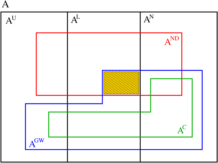
Figure 1: Lattice fermionic actions. Indicated are the sets with following properties: $A$ - hypercubic symmetries, gauge invariance, relativistic classical continuum limit; $A^{U}$ - ultralocal, $A^{L}$ - local but not ultralocal, $A^{N}$ - nonlocal, $A^{ND}$ - no doublers, $A^{C}$ - naive chiral symmetry, $A^{GW}$ - GWL symmetry.

We would also like to stress that weak non-ultralocality and strong non-ultralocality are two independent statements in the sense that one does not follow from the other. In this respect it should be pointed out that while non-ultralocality of GWL transformations applies regardless of doubling and does not apply for actions with naive chiral symmetry, non-ultralocality of GW actions is only necessary for doubler-free theories and actions with naive chiral symmetry represent no exception for this case.

Acknowledgements: I. H. and C. T. B. are grateful to William Fulton for his interest, help and support regarding Lemma 4. R. M. would like to acknowledge useful input and conversations with Dan Burghelea. I. H. benefited from communications with Pavel Bóna, Martin Niepel, František Marko, Arthur Mattuck and Andrei Rapinchuk, as well as from many pleasant discussions with Ziad Maassarani and Hank Thacker. We also thank Ziad for reading the manuscript.

Appendix A Local Symmetric Operators

The elements of the set ${{\twelvefrak G}^{sl}}$ satisfy three requirements defined below:

Definition 8

(Locality) Operator ${\bf G}$ is said to be local if there are positive real constants $c$, $\delta$ such that all its Clifford components ${\bf G}^{a}$ satisfy

$$|{\bf G}^{a}_{m,n}|\;<\;c\,e^{-\delta|m-n|}\qquad\quad\forall m,n$$

Here $|m-n|$ denotes the Euclidean norm of $m-n$.

Definition 9

(Translation Invariance) Operator ${\bf G}$ is said to be translationally invariant if all its Clifford components ${\bf G}^{a}$ satisfy

$${\bf G}_{m,n}^{a}={\bf G}_{0,n-m}^{a}\equiv g_{n-m}^{a}\qquad\quad\forall m,n$$

Definition 10

(Hypercubic Invariance) Let ${\cal H}$ be an element of the hypercubic group in defining representation and $H$ the corresponding element of the representation induced on hypercubic group by spinorial representation of $O(d)$. Operator ${\bf G}$ is said to have hypercubic invariance if for arbitrary ${\cal H}$, $m$, $n$ we have

$${\bf G}_{n,m}\;=\;H^{-1}{\bf G}_{{\cal H}n,{\cal H}m}\,H$$

In the Fourier space, we can directly define:

Definition 11

(Set ${{\twelvefrak G}^{sl}}$) Let $G^{a}(p),\;a=1,2,\ldots 2^{d}$, are the complex valued functions of real variables $p_{\mu}$, and let $G(p)$ be the corresponding matrix function constructed as in Eq. (3). We say that $G(p)$ belongs to the set ${{\twelvefrak G}^{sl}}$ if:

$(\alpha)$

Every $G^{a}(p)$ is an analytic function with period $2\pi$ in all $p_{\mu}$.

$(\beta)$

For arbitrary hypercubic transformation ${\cal H}$ it is true identically that

$$G(p)\;=\;\sum_{a=1}^{2^{d}}G^{a}(p)\Gamma^{a}\;=\;\sum_{a=1}^{2^{d}}G^{a}({\cal H}p)H^{-1}\Gamma^{a}H$$ (22)

Arbitrary hypercubic transformation ${\cal H}$ can be decomposed into products of reflections of single axis (${\cal R}_{\mu}$) and exchanges of two different axis (${\cal X}_{\mu\nu}$). Transformation properties of the elements of the Clifford basis are determined by the fact that $\gamma_{\mu}$ transforms as a vector. In particular

$$R_{\nu}^{-1}\gamma_{\mu}R_{\nu}\;=\;\cases{-\gamma_{\mu},&if $\mu=\nu$;\cr\gamma_{\mu},&if $\mu\neq\nu$\cr}$$

and

$$X_{\rho\sigma}^{-1}\gamma_{\mu}X_{\rho\sigma}\;=\;\cases{\gamma_{\sigma},&if $\mu=\rho$;\cr\gamma_{\rho},&if $\mu=\sigma$;\cr\gamma_{\mu},&otherwise\cr}$$

where $R_{\mu},X_{\mu\nu}$ are the spinorial representations of ${\cal R}_{\mu},{\cal X}_{\mu\nu}$. The elements of the Clifford basis naturally split into groups with definite transformation properties and the hypercubic symmetry thus translates into definite algebraic requirements on functions $G^{a}(p)$.

Appendix B Locality and Analyticity

Proposition 2

Let $G(p)$ be a complex function of single variable periodic with $2\pi$, and forming a Fourier pair with the sequence of complex numbers $\{g_{n}\,;\,n=0,\pm 1,\pm 2\ldots\}$, i.e.

$$G(p)\;=\;\sum_{n=-\infty}^{\infty}g_{n}e^{i\,n\,p}\;\equiv\;g_{0}+g_{1}e^{i\,p}+g_{-1}e^{-i\,p}+g_{2}e^{i\,2\,p}+g_{-2}e^{-i\,2\,p}+\ldots$$

and

$$g_{n}\;=\;{1\over{2\pi}}\int_{-\pi}^{\pi}dp\,e^{-i\,n\,p}\;G(p)$$

Then the following two statements are equivalent:

(a) There exist $c>0$,$\,\delta>0$ such that $\,\mid g_{n}\mid\;<\;c\,e^{-\delta\,|n|},\;\forall\,n$.

(b) There exists $\Delta>0$, such that $G(p)$ is analytic in the complex strip $\mid Im(p)\mid<\Delta$.

Proof. We first show that (a) implies (b). Consider the change of variables $z=e^{ip}$. Then $G=g(e^{ip})$ where the function $g$ is defined by

$$g(z)=g_{0}+g_{1}z+g_{-1}z^{-1}+g_{2}z^{2}+g_{-2}z^{-2}+\cdots$$

We split this up as $g(z)=h(z)+k(z)$ where

$$h(z)=g_{0}+g_{1}z+g_{2}z^{2}+\ldots\qquad\quad k(z)=g_{-1}z^{-1}+g_{-2}z^{-2}+\ldots$$

Condition (a) simply says that $|g_{n}|<c\beta^{-|n|}$ where $\beta>1$, implying that $h(z)$ has a radius of convergence strictly greater than $1$. Similarly, if we further change the variable $z=1/t$ in $k(z)$, so that $l(t)=k(1/t)$, we can infer that $l(t)$ too has a radius of convergence strictly greater than $1$. The above conclusions prove that $g(z)$ is analytic in an annulus containing the unit circle of the complex plane. Consequently, $G(p)=g(e^{ip})$ is a composition of two analytic maps, implying analyticity in the complex strip as desired in (b).

Next we show that (b) implies (a). Consider arbitrary $0<\rho<\Delta$. We will integrate in the complex plane along the rectangular contour ${\cal C}$ with the following line segments: ${\cal C}_{1}$ from point $(-\pi,0)$ to point $(\pi,0)$, $\,{\cal C}_{2}$ from $(\pi,0)$ to $(\pi,-\rho)$, $\,{\cal C}_{3}$ from $(\pi,-\rho)$ to $(-\pi,-\rho)$, and $\,{\cal C}_{4}$ from $(-\pi,-\rho)$ to $(-\pi,0)$.

Let us assume that $n\geq 0$. According to Cauchy theorem, we have

$$\int_{{\cal C}}dp\,e^{-i\,n\,p}\;G(p)\;=\;0\;=\;\int_{{\cal C}_{1}}\,+\,\int_{{\cal C}_{2}}\,+\,\int_{{\cal C}_{3}}\,+\,\int_{{\cal C}_{4}}$$

Since $G(p)$ is periodic with $2\pi$, the contributions from the integrals along ${\cal C}_{2}$ and ${\cal C}_{4}$ will cancel each other and we thus obtain

$$\int_{{\cal C}_{1}}dp\,e^{-i\,n\,p}\;G(p) = \int_{-\pi}^{\pi}dt\,e^{-i\,n\,t}\;G(t)\;=\;-\int_{{\cal C}_{3}}dp\,e^{-i\,n\,p}\;G(p)\;=\;$$

$$= \int_{-\pi}^{\pi}dt\,e^{-i\,n\,(t-i\rho)}\;G(t-i\rho)\;=\;e^{-n\,\rho}\,\int_{-\pi}^{\pi}dt\,e^{-i\,n\,t}\;G(t-i\rho)$$

Finally, $G(p)$ is bounded on the path of the last integral due to analyticity, and we thus have

$$\mid g_{n}\mid\quad=\quad\mid{1\over{2\pi}}\int_{-\pi}^{\pi}dt\,e^{-i\,n\,t}\;G(t)\mid\quad\leq\quad e^{-n\,\rho}\max_{t\in[-\pi,\pi]}\mid G(t-i\rho)\mid$$

Similarly if $n<0$, then we will use the rectangular integration contour in the upper half of the complex plane, yielding an analogous bound. Together, this then implies (a) as claimed.   

Appendix C Proof of Lemma 1

Proof. Let us denote the set of indices $u^{\rho}\equiv\{1,2\ldots\rho\}$ for arbitrary positive integer $\rho$. Clifford basis can be subdivided into non–intersecting subsets $\Gamma=\cup_{j}\Gamma_{(j)}$, where $\Gamma_{(j)}$, $j=0,1,\ldots,d$, contains the elements that can be written as the product of $j$ gamma-matrices. In particular, $\Gamma_{(0)}=\{\,{\twelvebb I}\,\}$, $\Gamma_{(1)}=\{\,\gamma_{\mu},\;\mu\in u^{d}\,\}$, and so on. With the appropriate convention on ordering of gamma–matrices in the definition of $\Gamma^{a}$, we can then rewrite the Clifford decomposition of $G(p)$ in the form

$$G(p)\;=\;\sum_{j=0}^{d}\sum_{\mu_{1},\mu_{2}\ldots\mu_{j}\atop\mu_{1}<\mu_{2}\ldots<\mu_{j}}F_{\mu_{1},\mu_{2}\ldots\mu_{j}}(p)\,\gamma_{\mu_{1}}\gamma_{\mu_{2}}\ldots\gamma_{\mu_{j}}\,,\qquad\quad\mu_{i}\in u^{d}$$ (23)

We will concentrate on contributions to ${\overline{G}}(q)$ originating from subsets $\Gamma_{(j)}$, where $j\geq 2$. Consider a single term in decomposition (23) from this group, specified by the set of indices $v\equiv\{\mu_{1},\mu_{2}\ldots\mu_{j}\}\neq u^{2}$. Then there exists element $\mu\in v$, such that $\mu\notin u^{2}$. Under reflection ${\cal R}_{\mu}$ through the corresponding axis, we have $R_{\mu}^{-1}\,\gamma_{\mu_{1}}\gamma_{\mu_{2}}\ldots\gamma_{\mu_{j}}\,R_{\mu}\,=\,-\gamma_{\mu_{1}}\gamma_{\mu_{2}}\ldots\gamma_{\mu_{j}}\,.$ Hypercubic symmetry of $G(p)$ then requires that $F_{\mu_{1},\mu_{2}\ldots\mu_{j}}({\cal R}_{\mu}p)=-F_{\mu_{1},\mu_{2}\ldots\mu_{j}}(p)\,.$ However, since $\mu\notin u^{2}$, the restricted variable $\overline{p}$ under $\Sigma^{2}$ satisfies ${\cal R}_{\mu}\overline{p}=\overline{p}$, and hence

$${\overline{F}}_{\mu_{1},\mu_{2}\ldots\mu_{j}}(q)\;\equiv\;F_{\mu_{1},\mu_{2}\ldots\mu_{j}}(\overline{p})\;=\;-F_{\mu_{1},\mu_{2}\ldots\mu_{j}}(\overline{p})\;=\;0$$

Consequently, the only Clifford element contributing from this group is $\gamma_{1}\gamma_{2}$ (when $v=u^{2}$), and the form (6) follows.

Analyticity, periodicity and relations (7-9) for functions $X(q),Y_{\mu}(q),Z(q)$ follow from corresponding properties of unrestricted operator.   

Appendix D Proof of Lemma 2

Proof. Since $G(p)$ is ultralocal, the Clifford components of ${\overline{G}}(q)$ have finite number of Fourier terms. Then there exists a non-negative integer $N$, such that when grouping together the Fourier terms related by reflection properties in (7-9) of Lemma 1, the Fourier expansions can be written in the form

$$X(q_{1},q_{2}) = \sum_{n_{1}=0}^{N}\sum_{n_{2}=0}^{N}x_{n_{1}n_{2}}\cos n_{1}q_{1}\cos n_{2}q_{2}$$

$$Y_{1}(q_{1},q_{2}) = \sum_{n_{1}=1}^{N}\sum_{n_{2}=0}^{N}y_{n_{1}n_{2}}\sin n_{1}q_{1}\cos n_{2}q_{2}\;=\;Y_{2}(q_{2},q_{1})$$

$$Z(q_{1},q_{2}) = \sum_{n_{1}=1}^{N}\sum_{n_{2}=1}^{N}z_{n_{1}n_{2}}\sin n_{1}q_{1}\sin n_{2}q_{2}$$

Furthermore, the exchange properties in (7) and (9) imply that $x_{n_{1},n_{2}}=x_{n_{2},n_{1}}$, while $z_{n_{1},n_{2}}=-z_{n_{2},n_{1}}$. Using the formulas for trigonometric functions of multiple arguments, namely

$$\sin nx\;=\;\sin x\,\Biggl{[}\,2^{n-1}\cos^{n-1}x - {{n-2}\choose 1}2^{n-3}\cos^{n-3}x\;+\;{{n-3}\choose 2}2^{n-5}\cos^{n-5}x$$

$$- {{n-4}\choose 3}2^{n-7}\cos^{n-7}x\;+\;\ldots\;\Biggr{]}$$

and

$$\cos nx\;=\;2^{n-1}\cos^{n}x - \frac{n}{1}\,2^{n-3}\cos^{n-2}x\;+\;\frac{n}{2}\,{{n-3}\choose 1}2^{n-5}\cos^{n-4}x$$

$$- \frac{n}{3}\,{{n-4}\choose 2}2^{n-7}\cos^{n-6}x\;+\;\ldots$$

the forms (10) directly follow, together with the exchange symmetry properties.   

Appendix E Refined Position of the Doubler

Proposition 3

Let $G(x,y,z)\in{\twelvebb C}\,[x,y,z]$ be homogeneous polynomial, such that $G(0,0,1)\neq 0$. Let further

$$B(x,y,z)\;\equiv\;x(z-x)\;G^{2}(x,y,z)+y(z-y)\;G^{2}(y,x,z)$$

If $F(x,y,z)P(x,y,z)\,=\,B(x,y,z)$ is arbitrary polynomial factorization such that

$$F(0,0,1)=0\qquad\qquad\quad P(0,0,1)\neq 0$$

then the projective algebraic curve $\Gamma_{F}$ passing through $(0,0,1)$ must also pass through $(1,1,1)$.

Proof. We are dealing with the special case of Proposition 1, given by $G_{1}(x,y)=G_{2}(y,x)=G(x,y)$, and all the arguments of the the proof in section 4.2.3 are valid here as well. Using the notation defined there and setting ${\mathbf{a}}_{1}=(0,0,1)\in\tilde{{\cal Z}}_{0}$ we have in particular

$$\sum_{{\mathbf{a}}\in\tilde{{\cal Z}}_{0}}i(\Gamma_{F},\Gamma_{F_{1}},{\mathbf{a}})\;=\;0\pmod{2}\qquad\qquad\qquad i(\Gamma_{F},\Gamma_{F_{1}},{\mathbf{a}}_{1})=1$$ (24)

We will show below that for ${\mathbf{a}}_{2}=(1,0,1),\,{\mathbf{a}}_{3}=(0,1,1)$ it is now true in addition that

$$i(\Gamma_{F},\Gamma_{F_{1}},{\mathbf{a}}_{2})\,+\,i(\Gamma_{F},\Gamma_{F_{1}},{\mathbf{a}}_{3})\,=\,0\pmod{2}$$ (25)

However, denoting ${\mathbf{a}}_{4}=(1,1,1)$ we have $\tilde{{\cal Z}}_{0}=\{{\mathbf{a}}_{1},{\mathbf{a}}_{2},{\mathbf{a}}_{3},{\mathbf{a}}_{4}\}$ and so (24), (25) imply that $i(\Gamma_{F},\Gamma_{F_{1}},{\mathbf{a}}_{4})=1\pmod{2}$. That proves the claim of the proposition.

To show (25), it is sufficient to concentrate on irreducible $\Gamma_{F}$. This is because such $\Gamma_{F}$ is unique and all the reducible ones will thus contain it. The uniqueness of irreducible $\Gamma_{F}$ follows from the fact that if there were at least two, then $\mathop{\rm ord}_{x,y}(B(x,y,z))$ would also have to be at least two, which is not the case. This also means that the corresponding $F(x,y,z)$ is symmetric in $x,y$. Indeed, if it were not, then the polynomial $F(y,x,z)$ would define another component of $\Gamma_{B}$ running through the point $(0,0,1)$ thus contradicting the uniqueness.

Assuming the above, consider arbitrary branch $\gamma=(\mu(t),\nu(t),1)$ of $\Gamma_{F}$, centered at ${\mathbf{a}}_{2}$. Due to symmetry in $x,y$ there is a corresponding branch $\gamma^{\prime}=(\nu(t),\mu(t),1)$ centered at ${\mathbf{a}}_{3}$. Using the fact that $\mathop{\rm ord}_{t}(\mu)=\mathop{\rm ord}_{t}(1-\nu)=0$ and $\mathop{\rm ord}_{t}(\nu)>0,\;\mathop{\rm ord}_{t}(1-\mu)>0$ we have

$$i(\gamma,\Gamma_{F_{1}},{\mathbf{a}_{2}})={\mathop{\rm ord}}_{t}(\mu(1-\mu))={\mathop{\rm ord}}_{t}(1-\mu)\qquad\quad i(\gamma^{\prime},\Gamma_{F_{1}},{\mathbf{a}_{3}})={\mathop{\rm ord}}_{t}(\nu(1-\nu))={\mathop{\rm ord}}_{t}(\nu)$$

while at the same time

$${\mathop{\rm ord}}_{t}(1-\mu)+{\mathop{\rm ord}}_{t}(\nu)\,=\,{\mathop{\rm ord}}_{t}(\mu(1-\mu)\nu(1-\nu))\,=\,{\mathop{\rm ord}}_{t}(F_{1}F_{2})\,=\,0\pmod{2}$$

The last two equalities relate to substituting $(x,y,z)\rightarrow(\mu(t),\nu(t),1)$ in $F_{1}\,,F_{2}$, and using eq. (13) which is valid for arbitrary branch $\gamma$ of $\Gamma_{F}$. It follows that $i(\gamma,\Gamma_{F_{1}},{\mathbf{a}}_{2})+i(\gamma^{\prime},\Gamma_{F_{1}},{\mathbf{a}}_{3})$ is even for arbitrary pair $(\gamma,\gamma^{\prime})$, implying (25).

References

- [1] L. Karsten and J. Smit, Nucl. Phys. B183 (1981) 103.
- [2] H. B. Nielsen and M. Ninomiya, Phys. Lett. B105 (1981) 219; Nucl. Phys. B185 (1981) 20[E: B195 (1982) 541].
- [3] P. Ginsparg and K. Wilson, Phys. Rev. D25 (1982) 2649.
- [4] P. Hasenfratz, Nucl. Phys. B525 (1998) 401.
- [5] S. Chandrasekharan, Phys.Rev. D60 (1999) 074503.
- [6] H. Neuberger, Phys. Lett B417 (1998) 141; Phys. Lett. B427 (1998) 353.
- [7] P. Hernández, K. Jansen and M. Lüscher, Nucl.Phys. B552 (1999) 363.
- [8] M. Lüscher, Phys. Lett. B428 (1998) 342.
- [9] I. Horváth, Phys. Rev. D60 (1999) 034510.
- [10] I. Horváth, Phys. Rev. Lett. 81 (1998) 4063.
- [11] I. Horváth, hep-lat/9912030.
- [12] W. Bietenholz, hep-lat/9901005 v3.
- [13] I. Horváth, hep-lat/0003030.
- [14] A. Seidenberg, “Elements of the Theory of Algebraic Curves”, Addison-Wesley, 1968.
- [15] B. L. van der Waerden, “Einführung in die Algebraische Geometrie”, Springer, Berlin, 1939.