SWAT/00/260

DESY 00-083

June 2000

NUMERICAL STUDY OF DENSE ADJOINT MATTER

IN TWO COLOR QCD

Simon Hands^a, István Montvay^b,c, Susan Morrison^a Manfred Oevers^d,

Luigi Scorzato^a and Jonivar Skullerud^b

^aDepartment of Physics, University of Wales Swansea,

Singleton Park, Swansea SA2 8PP, U.K.

^bTheory Division, DESY, Notkestrasse 85, D-22603 Hamburg, Germany.

^cCenter for Computational Physics, University of Tsukuba,

1-1-1 Tennodai, Tsukuba-shi, Ibariki-ken 305-8577, Japan.

^dDepartment of Physics and Astronomy, University of Glasgow,

Glasgow G12 8QQ, U.K.

Abstract

We identify the global symmetries of SU(2) lattice gauge theory with $N$ flavors of staggered fermion in the presence of a quark chemical potential $\mu$, for fermions in both fundamental and adjoint representations, and anticipate likely patterns of symmetry breaking at both low and high densities. Results from numerical simulations of the model with $N=1$ adjoint flavor on a $4^{3}\times 8$ lattice are presented, using both hybrid Monte Carlo and Two-Step Multi-Boson algorithms. It is shown that the sign of the fermion determinant starts to fluctuate once the model enters a phase with non-zero baryon charge density. HMC simulations are not ergodic in this regime, but TSMB simulations retain ergodicity even in the dense phase, and in addition appear to show superior decorrelation. The HMC results for the equation of state and the pion mass show good quantitative agreement with the predictions of chiral perturbation theory, which should hold only for $N\geq 2$. The TSMB results incorporating the sign of the determinant support a delayed onset transition, consistent with the pattern of symmetry breaking expected for $N=1$.

PACS: 11.10.Kk, 11.30.Fs, 11.15.Ha, 21.65.+f

Keywords: Monte Carlo simulation, chemical potential, diquark condensate

1 Introduction

In QCD it is believed that as the baryon density rises the degrees of freedom providing the most suitable description change from being “hadronic”, ie. composite states such as protons and neutrons, to being “partonic”, ie. quarks and gluons. This change may well be signalled by a phase transition as the appropriate thermodynamic variable, the baryon chemical potential $\mu$, is raised. Recent theoretical speculation [1, 2, 3] suggests that the ground state of strongly-interacting quark matter at high density may be more exotic than initially thought, for instance existing in a superconducting and/or superfluid state due to the condensation of diquark pairs at the Fermi surface via a BCS instability. In such a state the SU(3) color gauge group is spontaneously broken by a dynamical Higgs mechanism; in the language of condensed-matter physics this is the Meissner effect. As well as being of intrinsic theoretical interest, the behaviour of strongly-interacting matter at extreme densities is of fundamental importance both to nuclear physics and in understanding compact astrophysical objects such as neutron stars.

Unfortunately, it is difficult to apply the most reliable calculational tool for QCD, lattice gauge theory, directly to this problem. The reason is that once $\mu\not=0$, the anti-hermitian property of the Euclidian Dirac operator $D$ governing the motion of the quarks $q$ and anti-quarks $\bar{q}$ in the presence of the color field is spoiled, with the result that the functional measure $\mbox{det}M$, with $M\equiv D(\mu)+m$ where $m$ is the quark mass, is no longer positive definite. To apply the normal Monte Carlo method of importance sampling the path integral, the determinant must be split into a modulus and a phase; importance sampling is then done with respect to a measure $|\mbox{det}M|$, and $\mbox{arg(det}M)$ is incorporated with the observable:

$$\langle O\rangle={{\langle\langle O\,\mbox{arg(det}M)\rangle\rangle}\over{\langle\langle\mbox{arg(det}M)\rangle\rangle}},$$ (1.1)

where $\langle\langle\ldots\rangle\rangle$ denotes the expectation value with respect to the positive real measure. Now, the denominator of (1.1) is in effect a ratio of the partition functions of two different theories, one the true theory and the other an artificial one with a positive real measure: it should thus scale as $\exp(-\Delta F)$, where the free energy difference between the theories $\Delta F$ is an extensive quantity. The number of states to be sampled before estimators of observables converge therefore in general rises exponentially with the system volume. This is the origin of the notorious ‘sign problem’.

We can gain physical insight into the sign problem by considering standard QCD simulation algorithms such as the hybrid Monte Carlo (HMC) algorithm, which use a positive definite measure $\mbox{det}M^{\dagger}M$. The $M^{\dagger}$ has the effect of introducing “conjugate quarks” $q^{c}$ transforming in the conjugate representation of the color group [4]. In general the presence of light gauge invariant bound $qq^{c}$ states carrying net baryon number in the spectrum results in unphysical behaviour for $\mu\not=0$, eg. a premature “onset” transition between the vacuum and nuclear matter at $\mu_{o}\sim O(m_{\pi})$, the pion mass, which if chiral symmetry is spontaneously broken is much smaller than the constituent quark mass scale at which the transition is expected. There are, however, two strongly-interacting model theories where conjugate quarks can be tolerated. First consider the Nambu–Jona-Lasinio (NJL) model, long used as an effective theory for strong interactions; for sufficiently strong coupling it displays chiral symmetry breaking, signalled by a non-vanishing condensate $\langle\bar{q}q\rangle$ and the development of a constituent quark mass greatly exceeding the current quark mass $m$, together with a triplet of light mesonic (ie. $q\bar{q}$) pion states via Goldstone’s theorem. Conjugate quarks in numerical simulations of the NJL model are harmless because the diagrams responsible for the tight binding and small mass of the pions are only accessible in $q\bar{q}$ channels [5].

Next, consider non-abelian gauge theory in which the color group is SU(2) rather than the physical SU(3). Over the years “Two Color QCD” has been used to study the strong interaction in a variety of different contexts, the main motivation being that the computer effort required is appreciably less. Once quarks are introduced, however, important physical differences become apparent. Because the matter representations are all either real or pseudoreal, there is no gauge quantum number distinguishing $q$ from $\bar{q}$, resulting in enhanced global flavor symmetries in which both $q\bar{q}$ meson and $qq$ baryon states appear in the same multiplet [6], and chiral $\langle\bar{q}q\rangle$ and diquark $\langle qq\rangle$ condensates are related by global rotations [7, 8, 9]. The lightest baryon is therefore degenerate with the pion, and the onset chemical potential vanishes as $\mu_{o}\propto\surd m$ in the chiral limit. The same features ensure $\mbox{det}M(\mu)$ is real, and hence the theory simulable using standard algorithms [8, 10].

Our motivations for studying Two Color QCD with adjoint quarks are twofold. Firstly, as we shall demonstrate, the pattern of symmetry breaking anticipated for gauge theories with quarks in real or pseudoreal representations of the gauge group differs between continuum [9] and staggered lattice fermions [8]. There are good reasons, therefore, for considering the model with adjoint rather than fundamental quarks to be the most ‘QCD-like’ of the lattice models; in particular it has gauge invariant spin-$1\over 2$ states in its spectrum, for $N=1$ quark flavors no baryonic Goldstone modes are expected, and it could potentially have a superconducting ground state at high density. Secondly, for an odd number of flavors the functional measure, though real, is not positive definite. The model thus has a potential sign problem of a simpler form than QCD in that only sectors having opposite sign, rather than a continuum of phases, need be considered. It may thus be feasible to make progress using standard means, or at least expose physical distinctions between the two sectors.

Apart from the sign problem, which may almost be considered a problem of principle in the study of non-zero chemical potential, there are practical problems in using the HMC algorithm once $\mu\not=0$. For instance, the numerical effort required to invert the matrix $M(\mu)$ rises considerably as $\mu$ increases, due to the proliferation of complex eigenvalues with small modulus. This has encouraged us to study the performance of an alternative approach, the Two-Step Multi-Bosonic (TSMB) algorithm, in which $M$ is not inverted at all, but the effect of $\mbox{det}M$ incorporated by local Monte Carlo simulation over many auxiliary boson fields [11]. Our conclusion is that the TSMB algorithm may be by far the more effective approach, in terms of the cost to produce decorrelated configurations, in the high density phase. Moreover for the class of problem in which $\mbox{det}M$ is real but not positive our results suggest the HMC algorithm in its simplest form is not ergodic in the same region of parameter space, since it fails to change the sign of the determinant. The TSMB algorithm does not share this problem.

The remainder of the paper is organised as follows. In Section 2 we outline the global symmetries of the lattice model, and review the expected breaking pattern, for both adjoint and fundamental quarks. Operators for possible diquark condensates which form at high baryon density are discussed. We present a proof that $\mbox{det}M$ is real and positive for fundamental lattice quarks, but only real for adjoint. Finally issues concerning the continuum limit, which is problematic, are discussed. In section 3 we discuss both HMC and TSMB algorithms, and analyse their performance by considering the eigenvalue spectrum of $M$. It will be made clear that both sign problem and ergodicity are issues of practical importance once $\mu>\mu_{o}$, and that the TSMB approach is better suited to tackling them. In section 4 we present results of simulations using both algorithms. HMC simulations, confined to the sector of positive determinant, show clear evidence of an onset phase transition at $\mu_{o}\simeq m_{\pi}/2$ to a ground state with a non-zero density of baryon charge. The results moreover are in excellent agreement with analytic predictions obtained using chiral perturbation theory [9], which might be expected to hold for more than one quark flavor. By way of contrast the TSMB simulations, which take the determinant sign into account, show evidence that this onset transition is thereby delayed. Our conclusions and future plans are briefly outlined in Section 5.

2 Two Color QCD on the Lattice

2.1 Formulation and Symmetries at Low Density

In this section we review the formulation and symmetries of Two Color QCD with staggered lattice fermions in the presence of a chemical potential $\mu$, and compare them to those of the corresponding continuum models. In this way we hope to motivate the study of the model with $N=1$ flavor of adjoint quark as the most ‘QCD-like’ of the possibilities. The fermionic part of the lattice action is as follows:

$$S=\sum_{x,y}\bar{\chi}^{p}(x)D_{x,y}[U,\mu]\chi^{p}(y)+m\bar{\chi}^{p}(x)\delta_{x,y}\chi^{p}(y)\equiv\sum_{x,y}\bar{\chi}^{p}(x)M_{x,y}[U,\mu]\chi^{p}(y),$$ (2.1)

where the index $p$ runs over $N$ flavors of staggered quark, and $D$ is given by

$$D_{x,y}= {1\over 2} \sum_{\nu\not=0}\eta_{\nu}(x)\left(U_{\nu}(x)\delta_{x,y-\hat{\nu}}-U_{\nu}^{\dagger}(y)\delta_{x,y+\hat{\nu}}\right)$$ (2.2)

$$+ {1\over 2} \eta_{0}(x)\left(e^{\mu}U_{0}(x)\delta_{x,y-\hat{0}}-e^{-\mu}U_{0}^{\dagger}(y)\delta_{x,y+\hat{0}}\right).$$ (2.3)

The $\chi,\bar{\chi}$ are single spin component Grassmann objects, and the phases $\eta_{\mu}(x)$ are defined to be $(-1)^{x_{0}+\cdots+x_{\mu-1}}$.

In the case of fundamental quarks, the link matrices $U_{\mu}$ are complex $2\times 2$ matrices acting on isodoublet $\chi,\bar{\chi}$, and may be parametrised in terms of 3 real numbers $\alpha_{i}$ as $U=\exp(i\alpha_{i}\tau_{i})$, where $\tau_{i}$ are the Pauli matrices. Note that $\tau_{2}U\tau_{2}=U^{*}$. For adjoint quarks, the same group elements may be represented by real $3\times 3$ orthogonal matrices $O$ acting on isotriplet $\chi,\bar{\chi}$, given by

$$O_{ij}={1\over 2}\mbox{tr}(\tau_{i}U\tau_{j}U^{\dagger}).$$ (2.4)

In terms of the $\alpha_{i}$, $O=\exp(2i\alpha_{i}t^{i})$, where in this representation the generators $(t^{i})_{jk}=-i\varepsilon_{ijk}$ are hermitian, pure imaginary, and antisymmetric. For notational convenience we will continue to write the link variables as $U_{\mu}$ in either case.

On integration over $\chi$ and $\bar{\chi}$ the effective action $\exp(-S_{eff})=\mbox{det}^{N}M$ is obtained. Unlike three-color QCD with $\mu\not=0$, $\exp(-S_{eff})$ is real, since in the fundamental case $\mbox{det}M=\mbox{det}\tau_{2}M\tau_{2}=\mbox{det}M^{*}$, while in the adjoint case $M$ is manifestly real.

In the chiral limit $m=0$, the action has two manifest global symmetries:

$$\mbox{U}(N)_{e}:\;\;\;\chi_{e} \mapsto P\chi_{e}\;;\bar{\chi}_{o}\mapsto\bar{\chi}_{o}P^{\dagger}\;\;\;P\in\mbox{U}(N)$$

$$\mbox{U}(N)_{o}:\;\;\;\chi_{o} \mapsto Q\chi_{o}\;;\bar{\chi}_{e}\mapsto\bar{\chi}_{e}Q^{\dagger}\;\;\;Q\in\mbox{U}(N),$$ (2.5)

the $e/o$ subscripts denoting fields on even and odd sublattices respectively. However, it is straightforward to rearrange (2.1,2.3) using the Grassmann nature of $\chi,\bar{\chi}$ and the fact that $\eta_{\mu}(x\pm\hat{\mu})=\eta_{\mu}(x)$ to rewrite the action in this limit as

$$S={1\over 2}\sum_{xeven,\nu}\eta_{\nu}(x)\biggl{[}\bar{X}_{e}(x) \left(\matrix{e^{\mu\delta_{\nu,0}}&\cr&e^{-\mu\delta_{\nu,0}}\cr}\right) U_{\nu}(x)X_{o}(x+\hat{\nu})-$$ (2.6)

$$\bar{X}_{e}(x) \left(\matrix{e^{-\mu\delta_{\nu,0}}&\cr&e^{\mu\delta_{\nu,0}}\cr}\right) U_{\nu}^{\dagger}(x-\hat{\nu})X_{o}(x-\hat{\nu})\biggr{]}$$ (2.7)

where the fields $X,\bar{X}$ are given by

$$\bar{X}_{e}=(\bar{\chi}_{e},-\chi_{e}^{tr}\tau_{2})\;\;:\;\;X_{o}=\left(\matrix{\chi_{o}\cr-\tau_{2}\bar{\chi}_{o}^{tr}\cr}\right)$$ (2.8)

for fundamental quarks and

$$\bar{X}_{e}=(\bar{\chi}_{e},\chi_{e}^{tr})\;\;:\;\;X_{o}=\left(\matrix{\chi_{o}\cr\bar{\chi}_{o}^{tr}\cr}\right)$$ (2.9)

in the adjoint case. In the limit $\mu\to 0$ the U($N$)${}_{e}\otimes$U($N$)_o symmetry thus enlarges to U($2N$):

$$X_{o}\mapsto VX_{o}\;\;\bar{X}_{e}\mapsto\bar{X}_{e}V^{\dagger}\;\;\;V\in{\rm U}(2N).$$ (2.10)

Note that the U($2N$) group emerges because exact symmetries are non-anomalous in lattice formulations; for a continuum model with $N_{f}$ flavors the analogous symmetry enlargement is SU($N_{f})_{L}\otimes$SU($N_{f})_{R}\otimes$U(1)${}_{B}\to$SU($2N_{f}$) [6].

For a non-abelian gauge theory we expect spontaneous chiral symmetry breaking to occur at low density, signalled by the appearance of a chiral condensate $\langle\bar{\chi}\chi\rangle\not=0$, which in the first instance we will consider to have the same form as the bare quark mass term in (2.1). To determine the pattern of symmetry breaking it is helpful to recast the condensate in terms of $X,\bar{X}$: we find

$$\bar{\chi}\chi={1\over 2}\left[\bar{X}_{e}\left(\matrix{&1\kern-4.5pt1\cr 1\kern-4.5pt1&\cr}\right)\tau_{2}\bar{X}_{e}^{tr}+X_{o}^{tr}\left(\matrix{&1\kern-4.5pt1\cr 1\kern-4.5pt1&\cr}\right)\tau_{2}X_{o}\right]$$ (2.11)

in the fundamental case, and

$$\bar{\chi}\chi={1\over 2}\left[\bar{X}_{e}\left(\matrix{&1\kern-4.5pt1\cr-1\kern-4.5pt1&\cr}\right)\bar{X}_{e}^{tr}-X_{o}^{tr}\left(\matrix{&1\kern-4.5pt1\cr-1\kern-4.5pt1&\cr}\right)X_{o}\right]$$ (2.12)

for the adjoint. Here $1\kern-4.5pt1$ denotes the $N\times N$ unit matrix. The residual symmetry left unbroken by the condensate is that which leaves invariant respectively the symmetric/antisymmetric $2N\times 2N$ form. For $\mu=0$ we thus find

$$\mbox{fundamental}:\;\;\;\mbox{U}(2N)\to\mbox{O}(2N)\;\;\;\;\;\;\mbox{adjoint}:\;\;\;\mbox{U}(2N)\to\mbox{Sp}(2N).$$ (2.13)

This is remarkable in that it is the opposite of the breakdown in the continuum [6]:

$$\mbox{fundamental}:\;\;\;\mbox{SU}(2N_{f})\to\mbox{Sp}(2N_{f})\;\;\;\;\;\;\mbox{adjoint}:\;\;\;\mbox{SU}(2N_{f})\to\mbox{O}(2N_{f}).$$ (2.14)

In effect the rôles of fundamental and adjoint representations are reversed for staggered lattice fermions, a fact which has been noted several times over the years [12].

Next we identify the massless modes arising in the $m,\mu\to 0$ limit as a result of Goldstone’s theorem. For the fundamental case, the number of broken generators predicted by (2.13) is $N(2N+1)$. The case of $N=1$ fundamental quark has been analysed in [8] by considering infinitesimal rotations of the condensate (2.11) by $V_{\delta}=1\kern-4.5pt1+i\delta\lambda$, with $\lambda$ one of the U(2) generators $\{1\kern-4.5pt1,\tau_{i}\}$, and identifying the Goldstone mode with the coefficient of $O(\delta)$. The three Goldstones thus found are the familiar mesonic $0^{-}$ pion $\bar{\chi}\varepsilon\chi$ (where $\varepsilon(x)=(-1)^{x_{0}+x_{1}+x_{2}+x_{3}}$), and two scalar $0^{+}$ diquark states $\chi^{tr}\tau_{2}\chi,\,\bar{\chi}\tau_{2}\bar{\chi}^{tr}$. The $\pm$ superscripts here denote the symmetry of the state under the following lattice ‘parity’ symmetry:

$$x=(x_{0},x_{1},x_{2},x_{3}) \mapsto x^{\prime}=(x_{0},1-x_{1},1-x_{2},1-x_{3})$$ (2.15)

$$\chi(x)\mapsto(-1)^{x_{1}^{\prime}+x_{3}^{\prime}}\chi(x^{\prime}) \bar{\chi}(x)\mapsto(-1)^{x_{1}^{\prime}+x_{3}^{\prime}}\bar{\chi}(x^{\prime}).$$ ; (2.16)

For $m\not=0$, the three states remain degenerate [8], gaining masses $m_{\pi}\propto\surd m$ in accordance with standard PCAC arguments. In the case of adjoint quarks, the pattern (2.13) predicts $N(2N-1)$ Goldstones in general, and for $N=1$ the only Goldstone mode is the $0^{-}$ mesonic pion. The corresponding analysis for the continuum models has been performed for $N_{f}\geq 2$ with some care in [9]; the Goldstone counts are found to be $N_{f}(2N_{f}-1)-1$ (fundamental) and $N_{f}(2N_{f}+1)-1$ (adjoint). Modulo the mode destroyed by the U(1) axial anomaly, the reversal of fundamental and adjoint cases is clear. Another important distinction is that in the continuum the Goldstone spectrum always contains diquark states; in this respect the $N=1$ lattice adjoint model is special.

Now consider the effect of increasing $\mu$ from zero. The chemical potential has the effect of promoting a ground state containing baryonic matter, signalled by a non-zero value for the baryon number density

$$n={1\over 2}\left\langle\bar{\chi}(x)\eta_{0}(x)[e^{\mu}U_{0}(x)\chi(x+\hat{0})+e^{-\mu}U_{0}^{\dagger}(x-\hat{0})\chi(x-\hat{0})]\right\rangle.$$ (2.17)

At zero temperature $n$ thus serves as an order parameter for an onset phase transition occuring at some $\mu_{o}$ separating the vacuum from a state containing matter. A naive energetic argument would suggest that the onset transition should occur for a value of $\mu_{o}$ equal to the mass per baryon charge of the lightest particle carrying non-zero baryon number. For the models discussed in the previous paragraph in which some of the Goldstone modes are diquark states, those states will be the lightest baryons in the spectrum. Generically then, we expect $\mu_{o}\simeq m_{\pi}/2$ for most variants of Two Color QCD, which should be contrasted with the much larger value $m_{nucleon}/3$ expected in physical QCD. The exception is the lattice adjoint model with $N=1$. The fact that the lightest baryons are Goldstone modes and thus amenable to analysis by using Chiral Perturbation Theory ($\chi$PT) on an effective sigma model has been exploited in [9, 13] to calculate both Goldstone spectrum and equation of state of the continuum models as functions of $\mu$; the principal result is the prediction $\mu_{o}=m_{\pi}/2$.

2.2 Diquark Condensation at High Density

For a sufficiently high density of baryon charge, regardless of the nature of the bound states in the low energy spectrum, the fermionic nature of the quarks should ensure that the dominant degrees of freedom are governed by a Fermi-Dirac distribution. At zero temperature, all states will be occupied up to the Fermi energy $E_{F}$, which coincides with $\mu$ in the limit where inter-quark interactions can be neglected (for an asymptotically free theory we expect this approximation to improve as $\mu$ rises). The question now arises as to whether this simple description is unstable with respect to condensation of diquark pairs situated at antipodal points on the Fermi surface, resulting in an energy gap between the ground state and the lowest spin-$1\over 2$ excitation. For large $\mu$ this instability is generic provided the quark-quark interaction is attractive; that this is so for non-abelian gauge theories has been argued as arising from either gluon exchange [1], or instanton effects [2]. Physically, diquark condensation implies that fermion number and/or baryon charge is no longer conserved, and the ground state is a superfluid. For physical QCD, diquark pairs cannot be color singlet, so the condensation results in the phenomenon of color superconductivity, rendering some or all of the gluons massive via a dynamical Higgs mechanism [2, 3].

We now consider possible diquark condensates that might form in Two Color QCD. There are many possible diquark states that can be written down, and in the absence of a detailed dynamical calculation we have to proceed by making some ad hoc assumptions. We might imagine that the wavefunction of the $qq$ condensate should ideally be gauge invariant, spacetime scalar, and in the case of the lattice model, as local as possible in the $\chi$ fields, since non-local wavefunctions require the insertion of link variables to maintain gauge invariance, whose fluctuations will weaken the condensation. The most important consideration (and the only one which is inviolate [2, 14]) is that the condensate respects the Pauli Exclusion Principle, implying that the operator be antisymmetric with respect to exchange of quantum numbers between the quarks.

For Two Color Lattice QCD with fundamental quarks, a diquark operator which satisfies all of the above requirements is

$$qq_{\bf 2}={1\over 2}\left[\chi^{tr}(x)\tau_{2}\chi(x)+\bar{\chi}(x)\tau_{2}\bar{\chi}^{tr}(x)\right].$$ (2.18)

In fact [8], $qq_{\bf 2}$ is related to the chiral condensate $\bar{\chi}\chi$ by the U($2N$) symmetry (2.10), and as $\mu$ increases the chiral condensate (2.11) is in effect rotated into the diquark one. There is, however, a physical distinction between high and low density phases; with $N$ set to 1 and $m,\mu>0$ the U(2) symmetry is reduced to U(1)_B which is associated with conservation of baryon number. Condensation of $qq_{\bf 2}$ spontaneously breaks this residual symmetry resulting in an exactly massless Goldstone mode. Because of the change in the number of massless modes, there is a true phase separation between either the vacuum or a low density normal phase, and a high density superfluid phase. Preliminary Monte Carlo simulations have revealed a transition as $\mu$ is increased [8], and the associated condensation of $qq_{\bf 2}$ has been confirmed [15]. A superfluid condensate at high density is also found in both fundamental and adjoint continuum models [9]; here the sigma model approach permits a calculation of the spectrum and equation of state as a function of $\mu/m$, and predicts that $\langle qq\rangle$ and $n$ become non-zero at the same critical $\mu_{o}=m_{\pi}/2$, ie. there is no normal phase. Another important result is that for $\mu\gg m$ the pseudo-Goldstone states, which would have been massless in the SU(2$N_{f}$) symmetric limit, have mass $2\mu$ [9, 13].

Next we discuss the possibilities for Two Color Lattice QCD with adjoint quarks [16]. For $N\geq 2$, a diquark operator satisfying all of our ideal requirements can always be written down: for $N=2$ it reads

$$qq_{\bf 3}={i\over 2}\left[\chi^{p\,tr}(x)\varepsilon^{pq}\chi^{q}(x)+\bar{\chi}^{p}(x)\varepsilon^{pq}\bar{\chi}^{q\,tr}(x)\right],$$ (2.19)

where $p,q=1,2$ are explicit flavor indices. In fact, just as in the fundamental case, $qq_{\bf 3}$ is related to the adjoint chiral condensate (2.12) by a global symmetry, in this case the U(4) rotation given by

$$V={1\over 2}\left(\matrix{\phantom{i}P&iP^{tr}\cr iP&\phantom{i}P^{tr}\cr}\right)\;\;\;\mbox{with}\;\;\;P=\left(\matrix{1&-1\cr 1&\phantom{-}1\cr}\right).$$ (2.20)

Condensation of $qq_{\bf 3}$ breaks U(1)_B but leaves unbroken an SU(2) of isospin. Since there are diquark states among the 6 Goldstones expected from the breaking U(4) $\to$ Sp(4), we expect the usual scenario to apply, with a transition to a superfluid phase at $\mu_{o}=m_{\pi}/2$.

For $N=1$ the Exclusion Principle prevents us from writing a diquark operator satisfying all the requirements, since $\chi^{tr}(x)\chi(x)\equiv 0$. We have considered two possibilities. Firstly, a non-local operator which is gauge invariant and scalar under (2.16) is

$$qq_{\bf 3}^{\prime}={1\over 16}\sum_{\pm\mu}\eta_{\mu}(x)(-1)^{x_{\mu}}\left[\chi^{tr}(x)U_{\mu}(x)\chi(x+\hat{\mu})-\bar{\chi}(x)U_{\mu}(x)\bar{\chi}^{tr}(x+\hat{\mu})\right].$$ (2.21)

The $(-1)^{x_{\mu}}$ factor ensures that $qq_{\bf 3}^{\prime}$ is antisymmetric with respect to spatial exchange of $\chi$ fields. In terms of the $X,\bar{X}$ fields,

$$qq_{\bf 3}^{\prime}={1\over 8}\sum_{\pm\mu}\eta_{\mu}(x)(-1)^{x_{\mu}}\bar{X}_{e}(x)U_{\mu}(x)\left(\matrix{&-1\cr 1&\cr}\right)X_{o}(x+\hat{\mu}).$$ (2.22)

In the $m,\mu\to 0$ limit the global symmetries left unbroken by $\langle qq_{\bf 3}^{\prime}\rangle\not=0$ are a U(1)_ε symmetry,

$$X\mapsto e^{-i\alpha}X\;\;\;;\;\;\;\bar{X}\mapsto\bar{X}e^{i\alpha},$$ (2.23)

which is broken when $m\not=0$, and an O(2) symmetry rotating $\chi$ into $\bar{\chi}$:

$$X\mapsto QX\;\;\;;\;\;\;\bar{X}\mapsto\bar{X}Q^{tr}\;\;\;;\;\;\;Q=\left(\matrix{\phantom{-}\cos\theta&\sin\theta\cr-\sin\theta&\cos\theta\cr}\right).$$ (2.24)

The pattern of symmetry breaking is thus U(2)$\to$U(1)$\otimes$U(1)_ε, leaving two unbroken generators and hence two Goldstone modes, which turn out to be parity even meson and diquark states, the diquark remaining massless once $m,\mu>0$. Since for $m\not=0$ there are no exact Goldstones in the low density phase where chiral symmetry is broken, we once again predict a phase separation between a low density phase and a high density superfluid. Recalling, however, that the only Goldstone at low density is a $q\bar{q}$ meson, we are unable to apply the effective theory arguments of [9, 13], and in this case do not expect $\mu_{o}=m_{\pi}/2$.

Secondly, consider an operator which is local but not gauge-invariant:

$$qq_{sc}^{i}={1\over 2}\left[\chi^{tr}(x)t^{i}\chi(x)+\bar{\chi}(x)t^{i}\bar{\chi}^{tr}(x)\right],$$ (2.25)

whose consistency with the Exclusion Principle is now due to the antisymmetry of the generators $t^{i}$. Under a gauge transformation, $qq_{sc}^{i}$ transforms in the adjoint representation of SU(2),

$$qq_{sc}^{i}\mapsto O_{ij}qq_{sc}^{j},$$ (2.26)

which follows from the property $U^{-1}\lambda^{i}U=O_{ij}\lambda^{j}$, true for arbitrary representations generated by $\lambda^{i}$. Therefore $qq_{sc}^{i}$ acts like an adjoint Higgs field, and its condensation breaks the SU(2) color group to U(1), as in the Georgi-Glashow model of electroweak physics [17]. As the subscript implies, this is therefore a superconducting solution; ironically, in this case the superconducting phase is characterised (at least in perturbation theory) by a massless photon. Once again, because of the change in the number of massless particles between the low density confined phase and the high density superconducting phase, a true phase separation is expected, which is consistent with general properties of gauge theories with Higgs fields in the adjoint representation [19], and in possible contrast with the ‘color-flavor locked’ state anticipated in three-flavor QCD [3], where continuity between high and low density phases has been postulated [20].

2.3 The Sign of the Determinant

As discussed in subsection 2.1, it is straightforward to show that the path integral measure, proportional to $\mbox{det}M$, is real. To determine whether it is positive definite requires a more subtle argument. Let us first make some general observations:

• Lemma 1: let $M$ be any diagonalisable operator and $K$ be the complex conjugation operator. If there exists a unitary operator $T$ such that $[KT,M]=0$, then $\mbox{det}M$ is real.

• Proof: let $\psi$ be an eigenvector of $M$ with eigenvalue $\lambda$; then $\tilde{\psi}=KT\psi$ is an eigenvector with eigenvalue $\lambda^{*}$:

  $$M\psi=\lambda\psi\;\Rightarrow\;KTM\psi=KT\lambda\psi\;\Rightarrow\;MKT\psi=\lambda^{*}KT\psi\;\Rightarrow\;M\tilde{\psi}=\lambda^{*}\tilde{\psi};$$

  hence $\mbox{det}M$ is real, since the product over eigenvalues can be organised in complex conjugate pairs.

Now this does not imply that $\mbox{det}M$ is positive, since for real $\lambda$, $\tilde{\psi}$ might be proportional to $\psi$, and hence we cannot exclude the possible existence of non-degenerate real eigenvalues which may include an odd number of negative ones. To prove that $\psi$ and $\tilde{\psi}$ are linearly independent, we need $KT$ to have another property.

• Lemma 2: if $(KT)^{2}=-1$, $\psi$ and $\tilde{\psi}$ are linearly independent.

• Proof:

  $$\langle\psi|\tilde{\psi}\rangle=\langle\psi|KT\psi\rangle=\langle T\psi|TKT\psi\rangle=\langle(KT)^{2}\psi|KT\psi\rangle=-\langle\psi|\tilde{\psi}\rangle=0,$$

  where we have used $\langle\phi|\psi\rangle=\langle K\psi|K\phi\rangle$.

Hence if $[KT,M]=0$ and $(KT)^{2}=-1$, all real eigenvalues are doubly degenerate, and $\mbox{det}M>0$.

The square of the anti-unitary operator $KT$ determines the Dyson index $\beta$ of $M$, the case $(KT)^{2}=1$ implying $\beta=1$ and $(KT)^{2}=-1$ implying $\beta=4$ [9]. Physical QCD with three colors and fundamental quarks has no operator equivalent to $KT$, corresponding to $\beta=2$. Now let us identify the operator $T$ for both continuum and for staggered lattice fermions. In the continuum,

$$M=(\partial_{\nu}+ig\lambda^{i}A_{\nu}^{i})\gamma_{\nu}+\mu\gamma_{0}+m,$$ (2.27)

with $A_{\nu}^{i}$ the gauge potential and $\lambda^{i}$ the generator appropriate to the quark representation. We find

$$\mbox{fundamental:}\;\;\;T = C\gamma_{5}\otimes\tau_{2},\;\;(KT)^{2}=1\;\;\Rightarrow\beta=1;$$

$$\mbox{adjoint:}\;\;\;T = C\gamma_{5}\otimes 1\kern-4.5pt1,\;\;(KT)^{2}=-1\;\;\Rightarrow\beta=4.$$ (2.28)

Here, $C$ is the charge conjugation matrix defined by its operation on Euclidean hermitian $\gamma$-matrices: $C\gamma_{\mu}C^{-1}=-\gamma_{\mu}^{*}$. For staggered lattice fermions $M$ is given by (2.1,2.3), and

$$\mbox{fundamental:}\;\;\;T = \tau_{2},\;\;(KT)^{2}=-1\;\;\Rightarrow\beta=4;$$

$$\mbox{adjoint:}\;\;\;T = 1\kern-4.5pt1,\;\;(KT)^{2}=1\;\;\Rightarrow\beta=1.$$ (2.29)

Once again, we see the rôles of fundamental and adjoint representations reversed for staggered lattice fermions. We thus have a proof that the functional integral measure is positive definite for continuum adjoint quarks and fundamental lattice quarks. There is no such proof for continuum fundamental quarks and lattice adjoint quarks, and as we shall demonstrate in section 3.1, there are indeed isolated real eigenvalues and hence a sign problem for the adjoint lattice model at large chemical potential $\mu$.

2.4 The Continuum Limit

In this paper our viewpoint will be to study the lattice model in its own right, that is as a strongly coupled theory with the potential to show superfluid or superconducting properties at high density, and not to attempt either continuum or chiral limits. We have therefore focussed on the global symmetries appropriate to staggered fermions. This should not obscure the fact, however, that there are interesting issues related to the continuum limit whose resolution is still not clear. The model with $N$ flavors of staggered fermion should correspond to a continuum theory with $N_{f}=4N$ physical quark flavors. For the model with fundamental quarks, therefore, we expect the U(2$N$) global symmetry to enlarge to SU(8$N$), which is spontaneously broken by a chiral condensate to Sp(8$N$): for the adjoint model the corresponding pattern is SU(8$N)\to\mbox{O}(8N)$. Does the rôle reversal of fundamental and adjoint representations cease at some point? Since the behaviour of both is qualitatively similar in the continuum formulation, this is plausible [9]. On the other hand, we have argued that the lattice model with $N=1$ staggered flavor exhibits a distinct behaviour, with no premature onset transition, and the possibility of a superconducting condensate. If this were the case, would the superconducting phase survive the continuum limit? Above we also argued that the sign of the fermion determinant $\mbox{det}M$ is not positive in all cases, implying that it is important whether $N$ is even or odd, and once again continuum and lattice models have distinct behaviour.

Let us outline a possible route to resolving these issues. First consider the effect of extending the continuum operator $T$ of eqn. (2.3) by including the effects of a four-index flavor structure. One can then consider an operator

$$T^{\prime}=T\otimes\Gamma$$ (2.30)

where $\Gamma$ is a $4\times 4$ matrix acting on flavor; the case $\Gamma=C\gamma_{5}$ has the property that $(KT^{\prime})^{2}=-(KT)^{2}$, which would render the fermion determinant for 4 fundamental continuum flavors positive (as must clearly be the case). Next consider the form of the lattice $T$ operator (2.3) in a basis of fields $q^{\alpha a},\bar{q}^{\alpha a}$ carrying both a spinor index $\alpha$ and a flavor index $a$ (implicit in the staggered fermion approach), each taking values from 1 to 4 [21]. The appropriate structure is

$$T_{q}=C\gamma_{5}\otimes C\gamma_{5}\otimes\left\{\matrix{\tau_{2}\cr 1\kern-4.5pt1\cr}\right\},$$ (2.31)

where the first $C\gamma_{5}$ acts on the spinor index, the second on flavor, and the final $\tau_{2}$ ($1\kern-4.5pt1$) acts on color in the case of fundamental (adjoint) quarks. At non-zero lattice spacing, due to a term which is formally $O(a)$ when $M$ is expressed in the $q,\bar{q}$ basis [21], this is the only exact symmetry of the form (2.3,2.3); as we saw, $(KT_{q})^{2}=1$ for adjoint quarks, implying a possible sign problem. However, in the continuum limit we expect flavor symmetry to be restored, implying that $T^{\prime}_{q}$ with the second $C\gamma_{5}$ substituted by arbitrary $\Gamma$ will also define symmetries of $M$. The existence of merely one $T^{\prime}_{q}$ with $(KT^{\prime}_{q})^{2}=-1$ (eg. $\Gamma=1\kern-4.5pt1$) suffices to prove $\mbox{det}M$ positive due to degeneracy of real eigenvalues; we expect as a consequence an enlargement of the Goldstone manifold to recover the continuum symmetry prediction. Away from the continuum limit, these extra baryonic Goldstone modes remain massive due to lattice artifacts.

We can also examine the diquark condensates postulated in subsection 2.2 in terms of $q,\bar{q}$ [14]. In this representation the local diquark operators (2.18, 2.19, 2.26) take the form

$$qq={1\over 2}\left[q^{tr}(C\gamma_{5}\otimes C\gamma_{5}\otimes T)q+\bar{q}(C\gamma_{5}\otimes C\gamma_{5}\otimes T)\bar{q}^{tr}\right],$$ (2.32)

where the first operator in the tensor product in each term acts on spinor indices, the second on flavor, the third on gauge indices (or explicit flavor indices in the case of (2.19)), and all three are antisymmetric matrices. In the same basis the parity transformation (2.16) reads

$$q(x)\mapsto(\gamma_{0}\otimes\gamma_{5}\otimes 1\kern-4.5pt1)q(x^{\prime})\;\;\;;\;\;\;\bar{q}(x)\mapsto\bar{q}(x^{\prime})(\gamma_{0}\otimes\gamma_{5}\otimes 1\kern-4.5pt1).$$ (2.33)

We thus confirm that the first $C\gamma_{5}$ is consistent with the local condensates being spacetime scalars, the second $C\gamma_{5}$ implying that the condensates transform in the antisymmetric tensor representation of the continuum flavor SU(4) symmetry expected away from the chiral limit, which has dimension 6. The situation is different for the non-local condensate (2.21), which reads

$$qq_{\bf 3}^{\prime}=\sum_{\mu}q^{tr}(C\otimes C\gamma_{\mu}^{*}\otimes 1\kern-4.5pt1)q-\bar{q}(C\otimes C\gamma_{\mu}^{*}\otimes 1\kern-4.5pt1)\bar{q}^{tr}.$$ (2.34)

Invariance of $qq_{\bf 3}^{\prime}$ under parity depends on the non-trivial action of (2.33) on flavor, and in fact the spacetime structure of the operator implies that this condensate is pseudoscalar. The symmetry of $qq_{\bf 3}^{\prime}$ may be checked noting that $C\gamma_{\mu}^{*}$ is a symmetric matrix, in turn implying that this condensate transforms as a symmetric 10 of flavor SU(4). Without further detailed dynamical input, it is difficult to proceed; it may well prove that the route to the continuum is complicated, with several distinct phases found as the parameters $\beta$, $m$ and $\mu$ are tuned.

Finally, we note that because adjoint sources screen color four times more effectively than fundamental ones, asymptotic freedom is lost in Two Color QCD with $N_{f}$ massless adjoint quarks for $N_{f}=4N>11/4$, ie. even for $N=1$. Therefore in the chiral limit even the location of the continuum limit is a priori unknown; possible behaviours include a continuum limit described by a non-perturbative renormalisation group fixed point at some finite value of the gauge coupling $\beta_{c}$, or no interacting continuum limit existing at all. In section 4 we will demonstrate that these considerations are irrelevant at the values of $\beta$ and $m$ considered in our work.

2.5 Summary

In this section we have reviewed the formulation and symmetries of Two Color lattice QCD at length, and compared and contrasted it with corresponding continuum models. We conclude that the version of Two Color QCD which is most ‘QCD-like’ with respect to non-zero chemical potential $\mu$ and hence worthy of study, is that with $N=1$ flavor of staggered lattice fermion in the adjoint representation, for the following reasons:

• There are no Goldstone diquarks in the spectrum at zero density, and hence no reason to expect a premature onset transition at $\mu_{o}\simeq m_{\pi}/2$.

• The spectrum in the confined phase should contain gauge invariant fermionic bound states, either of a quark and a gluon, or of an odd number of quarks. Hence there is the possibility of a nuclear liquid phase, and the formation of a Fermi surface, before the restoration of chiral symmetry expected as $\mu$ is increased.

• The path integral measure is real but not positive definite for any odd $N$; that of QCD is complex. It may prove possible to expose the importance of configurations with non-positive definite $\mbox{det}M$ in the path integral with $\mu\not=0$.

• There is a possibility of a gauge-variant diquark condensation at high densities, leading to color superconductivity. No other lattice model capable of being studied with $\mu\not=0$ appears to share this feature [8, 14, 15].

It is conceivable that some or all of these factors are intimately linked.

3 Simulation Algorithms

We have studied Two Color lattice QCD with adjoint staggered fermions using two different simulation algorithms, the hybrid Monte Carlo (HMC) algorithm [22], and a Two-Step Multi-Bosonic (TSMB) algorithm [23]. Here we outline the two methods, and point out some important features of each.

3.1 The Hybrid Monte Carlo Algorithm

The HMC algorithm starts from an expression for the action $S$ in terms of bosonic auxiliary pseudofermion variables $\Phi$:

$$S={1\over 2}\sum_{x,y}\sum_{p=1}^{N}\Phi^{p\,tr}(x)(M^{tr}M)^{-1}_{x,y}[U,\mu]\Phi^{p}(y)-{\beta\over 2}\sum_{x,\mu<\nu}\mbox{Tr\,}U_{\mu\nu}(x),$$ (3.1)

where the fermion matrix $M$ is defined in (2.1,2.3), $\beta$ is the gauge coupling constant, and the trace over the plaquette is taken in the fundamental representation. In contrast to QCD, the $\Phi$ may be taken real, since $M$ is real. Gaussian integration over $\Phi$, which is convergent since the eigenvalues of $(M^{tr}M)^{-1}$ are real and positive, yields a factor proportional to

$$\exp(-S_{eff})=(\sqrt{\mbox{det}M^{tr}M})^{N}=|\mbox{det}M|^{N}.$$ (3.2)

This coincides with the correct functional measure $\mbox{det}^{N}M$ if $\mbox{det}M$ is positive. In this case HMC correctly simulates $N=1$ flavor of staggered lattice fermion. Note that for $\mu\not=0$, the usual trick of evaluating $(M^{tr}M)^{-1}$ on just even lattice sites, thus reducing the effective number of fermion degrees of freedom by a further factor of two, is not available since the chemical potential spoils the anti-hermitian form of $D$, the off-diagonal part of $M$.

It is instructive to analyse the performance of the algorithm by considering the eigenvalue spectrum of $M$. Because $D$ only connects even sites with odd and vice-versa, if $\psi(x)$ is an eigenvector with eigenvalue $\lambda=m+\kappa$, then so is $\varepsilon(x)\psi(x)$, with eigenvalue $\lambda=m-\kappa$. Because $D$ is a real matrix, if $\psi$ is an eigenvector with eigenvalue $\lambda$ then so is $\psi^{*}$ with eigenvalue $\lambda^{*}$. Now for $\mu=0$, the matrix $D$ is anti-hermitian, implying its eigenvalues are pure imaginary; we deduce that in this case the spectrum of $M$ lies along the line $\lambda=m+iz$, with $z$ real. For $\mu\not=0$, the symmetries between $\lambda$, $\lambda^{*}$ and $2m-\lambda$ persist, but now the spectrum swells out to occupy a roughly elliptical region of the complex plane, whose horizontal dimension grows with increasing $\mu$.

Figure 1: Eigenvalue spectrum from a $4^{3}\times 8$ lattice with $\beta=2.0$, $m=0.1$ and $\mu=0.35$. Note the mismatch in scale between real and imaginary axes.

The spectrum from a representative configuration is shown in Fig. 1. A feature of interest is that even once the spectrum has swelled out, an appreciable fraction of the eigenvalues remain on the line $\lambda=m+iz$; this contrasts with behaviour observed in three-color QCD, where all eigenvalues leave the line once $\mu\not=0$ [24], but is similar to the spectrum of the random matrix Dirac operator with $\mu\not=0$ and Dyson index $\beta=1$ (corresponding to a matrix $D$ with off-diagonal elements chosen from a chiral Gaussian Orthogonal Ensemble) [25]. Secondly, for this particular value of $\mu=0.35$ the spectrum has broadened sufficiently for the extremal eigenvalues to have negative real parts.

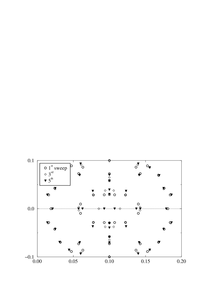
Figure 2: Spectral flow under HMC evolution.

The HMC algorithm works by evolving the $\{U\}$ fields in fictitious time $\tau$ for a period called a trajectory, whereupon the resulting configuration is accepted or rejected via a Metropolis step; the acceptance probability is related to how well the pseudo-Hamiltonian flow conserves energy. At the start of each trajectory the pseudofermion and conjugate momentum fields are refreshed from a Gaussian heat-bath, which ensures ergodicity in most cases. The trajectory length may be held constant or picked at random, but is usually chosen to be $O(1)$. We find, however, that once the eigenvalue occupation region has swelled to include the origin, the resulting presence of very small eigenvalues causes numerical instabilities, and necessitates smaller trajectory lengths — the data of Fig. 1 were generated using an average trajectory length of 0.18. An HMC update step acts on the configuration as a whole, and high acceptance is maintained by making a sequence of small changes: HMC is thus a small step-size algorithm. In Fig. 2 we show the spectral flow under HMC evolution in a small region close to the origin, starting from the configuration of Fig. 1 and evolving for five very short trajectories of length 0.003. For clarity only the eigenvalues from the first, third and fifth steps are shown. Note that there are a few eigenvalues which are real: a pair close to 0.1$\pm$0.08 on the first configuration, which increases to eight by the fifth. Close inspection reveals that between the first and third configurations a pair of eigenvalues jumps from the line $\lambda=m+iz$ at approximately $0.1\pm 0.03i$ to the real axis at $\simeq 0.1\pm 0.02$ — such processes change the number of real eigenvalues by $\pm 2$, and the number on the line $\lambda=m+iz$ by $\mp 2$. Between the third and fifth configurations, two pairs of conjugate eigenvalues coalesce and then move independently along the real axis at $\simeq 0.1\pm 0.04$ — this process changes the number of real eigenvalues by $\pm 4$. Finally between the third and fifth configurations we can also see pairs of eigenvalues coalesce and then move independently along $m+iz$ at $\simeq 0.1\pm 0.04i$, changing the number of eigenvalues on this line by $\pm 4$. All other eigenvalues in the region, at generic points in the complex plane, merely exhibit small fluctuations under HMC evolution. The symmetries between $\lambda$, $\lambda^{*}$ and $2m-\lambda$ are maintained at all times.

Fig. 2 demonstrates unambiguously the existence of non-degenerate real eigenvalues of $\lambda$, and the fact that there is always an even number of them. There is no obstruction in principle to there being an odd number of negative real eigenvalues, resulting in $\mbox{det}M<0$. However, since the processes discussed in the previous paragraph always create real eigenvalues in pairs at the same point, the only route to $\mbox{det}M<0$ can be if an isolated eigenvalue moves along the real axis and through the origin, forcing $\mbox{det}M$ to evolve smoothly through zero. In the neighbourhood of such a point the effective action $S_{eff}$ diverges, implying a strong repulsive force in the Hamiltonian flow, and hence a large kinetic barrier to changing the determinant’s sign. This barrier is a feature of any model in which $\mbox{det}M$ is real; in QCD, which has $\mbox{det}M$ complex, it should be straightforward to change the sign by moving through a sequence of configurations in which the phase of the determinant gradually increases from 0 to $\pi$.

Figure 3: Evolution of $|\ln\mbox{det}M|\times\mbox{sign}(\mbox{det}M)$ using HMC, quenched and TSMB updates on a $4^{3}\times 8$ lattice at $\beta=2.3$, $m=0.1$ and $\mu=0.6$.

In Fig. 3 we show evolution of $\ln\mbox{det}M$ for 40 representative configurations, each separated by 50 trajectories of average length 0.05. The simulation parameters have been chosen such that the left-hand edge of the spectrum extends well beyond the imaginary axis, so that we expect a non-vanishing probability of obtaining negative real eigenvalues. We see on inspection of the first, solid curve that HMC evolution does not appear to change the sign of $\mbox{det}M$. This could in principle be because the volume of configuration space with an odd number of real negative eigenvalues is very small; we can eliminate this possibility by considering a comparable sequence of quenched updates (dotted curve). In this case the sign of $\mbox{det}M$ is seen to change frequently, confirming that such configurations exist and are relatively easy to find. Moreover, if one of the configurations with $\mbox{det}M<0$ is then reequilibrated with HMC and allowed to evolve, we see that once again the sign remains stable and negative (dot-dashed curve); this behaviour is observed to persist for both signs for approaching 20000 trajectories. We reach two important conclusions:

• There are regions of parameter space with $\mu\not=0$ for which $\mbox{det}M$ can take negative values, ie. there is a sign problem.

• The kinetic barrier at the origin prevents the HMC algorithm from changing the sign of $\mbox{det}M$, and therefore from exploring the whole of the system’s configuration space: in other words, the HMC algorithm is not ergodic in this region of parameter space.

The sign problem is well-known [26] and can be addressed, at least in principle, by including the sign of $\mbox{det}M$ with the observable as in (1.1); this may be expected to be effective provided the average sign is significantly different from zero. The problem with ergodicity is less well-known — it can be anticipated in any model where $M$ is real but its eigenvalues $\lambda$ complex; another example which would be interesting to study is the lattice Gross–Neveu model with discrete Z₂ chiral symmetry [27]. Note that it remains a problem of principle for even $N$, since we can still classify a configuration by the number of negative real eigenvalues of $M$. It is an interesting open question whether or not the absence of transitions between odd and even sectors is of practical importance.

Despite its problems, we have made an extensive study of Two Color QCD using the HMC algorithm, and the results will be surveyed in section 4. We next turn to an algorithm which has the potential to overcome the ergodicity problem.

3.2 The Two-Step Multi-Bosonic Algorithm

For the Two-Step Multi-Bosonic algorithm [23] we also need a hermitian fermion matrix. First one might consider

$$\tilde{Q}(\mu)\equiv\varepsilon M(\mu)=\tilde{Q}(-\mu)^{\dagger},$$ (3.3)

but for non-zero chemical potential this is still not hermitian. Hermiticity may be achieved by doubling the matrix size:

$$\hat{Q}(\mu)\equiv\left(\begin{array}[]{cc}0&\tilde{Q}(-\mu)\\ \tilde{Q}(\mu)&0\end{array}\right)=\hat{Q}(\mu)^{\dagger}\ .$$ (3.4)

Following from

$$\hat{Q}(\mu)^{2} = \left(\begin{array}[]{cc}\tilde{Q}(-\mu)\tilde{Q}(\mu)&0\\ 0&\tilde{Q}(\mu)\tilde{Q}(-\mu)\end{array}\right)$$ (3.7)

$$= \left(\begin{array}[]{cc}M(\mu)^{\dagger}M(\mu)&0\\ 0&M(-\mu)^{\dagger}M(-\mu)\end{array}\right)$$ (3.10)

and noting that

$$\det M(\mu)=\det M(\mu)^{*}=\det M(-\mu),$$ (3.11)

(where the first equality holds because $M=D+m$ is real, the second because $D^{tr}(\mu)=-D(-\mu)$, and the spectrum of $D$ is symmetric about zero), we deduce

$$\det\hat{Q}(\mu)^{2}=\left\{\det M(\mu)\right\}^{4}\ ,\hskip 20.00003pt|\det M(\mu)|=\left\{\det\hat{Q}(\mu)^{2}\right\}^{1\over 4}\ .$$ (3.12)

In multi-bosonic representations of the fermion determinant [11] polynomials are used to approximate the necessary inverse powers of $x\equiv\hat{Q}(\mu)^{2}$ over some prescribed range $x\in[\epsilon,\lambda]$:

$$\frac{1}{x^{1\over 4}}\simeq P(x)\ ,\hskip 20.00003pt|\det M(\mu)|\simeq\frac{1}{\det P\left(\hat{Q}(\mu)^{2}\right)}\ .$$ (3.13)

This shows that in the present case the same polynomial approximations can be used as in recent numerical simulations of supersymmetric Yang Mills theory [28].

The usual way to represent the determinant of the polynomial in (3.13) is by functional integration over complex pseudofermion boson fields. Since the fermion matrix is real, it is also possible to use a real multi-bosonic representation, just as in the HMC case. For this we need a different polynomial approximation:

$$\frac{1}{x^{1\over 2}}\simeq\bar{P}(x)\ ,\hskip 20.00003pt|\det M(\mu)|\simeq\frac{1}{\left\{\det\bar{P}\left(\hat{Q}(\mu)^{2}\right)\right\}^{1\over 2}}\ .$$ (3.14)

Since the polynomial $\bar{P}(x)$ is supposed to have complex conjugate pairs of roots, one can decompose it, with an overall factor $r_{0}$, as

$$\bar{P}(\hat{Q}(\mu)^{2})=r_{0}\prod_{j}[\hat{Q}(\mu)^{2}+r_{j}]=r_{0}\prod_{j}[(\hat{Q}(\mu)+\mu_{j})^{2}+\nu_{j}^{2}]\ ,$$ (3.15)

with $\mu_{j}$, $\nu_{j}$ real. In order to achieve this form one has to choose the signs of the square roots of two complex conjugate roots appropriately: $r_{j}=(i\mu_{j}+\nu_{j})^{2},\ r_{j+1}=r_{j}^{*}=(-i\mu_{j}+\nu_{j})^{2}$. The multi-bosonic representation with real pseudofermion fields is then

$$\frac{1}{\left\{\det\bar{P}\left(\hat{Q}(\mu)^{2}\right)\right\}^{1\over 2}}\propto\int[d\Phi]\exp\left(-\sum_{jyx}\Phi_{y}^{j\,tr}[(\hat{Q}(\mu)+\mu_{j})^{2}+\nu_{j}^{2}]_{yx}\Phi_{x}^{j}\right)\ .$$ (3.16)

The polynomial orders for a sufficiently good approximation in (3.14) are typically somewhat higher than in (3.13) but the use of real fields has the advantage of taking half the storage and roughly half the arithmetic.

In the TSMB algorithm the polynomials in eqs. (3.13) and (3.14) are obtained by a product of lower order polynomials. The multi-bosonic representation is taken for the first factor $P^{(1)}_{n_{1}}(x)$ with a relatively low order $n_{1}$. This diminishes the storage requirements and improves autocorrelations. A better approximation of the fermion determinant is achieved by a second polynomial factor $P^{(2)}_{n_{2}}(x)$ of order $n_{2}$. In the gauge field update the effect of $P^{(2)}$ is taken into account stochastically. Another auxiliary polynomial $P^{(3)}_{n_{3}}(x)$ is also needed in this stochastic correction. The final precision in the approximation is achieved by reweighting the gauge configurations when evaluating expectation values. There a fourth polynomial $P^{(4)}_{n_{4}}(x)$ is used. For appropriate algorithms to obtain the necessary optimized polynomial approximations see [29]. A detailed description of the TSMB algorithm can be found in [30].

There are two reasons why the TSMB algorithm can overcome the ergodicity problem related to the zero of the fermion determinant discussed in section 3.1. First, the gauge field updates are performed by some large step-size algorithm, in our case the Metropolis algorithm. Second, the imperfect approximations near the zero of the determinant open a “hole” where the tunnelling between the sectors of differing determinant sign is facilitated. The small error in the evaluation of expectation values due to the imperfection of the approximation can be removed by the reweighting step [31]. In Fig. 3 we show as a dashed line the evolution of $|\ln\mbox{det}M|\times\mbox{sign(det}M)$ (for the uncorrected $M$), using a TSMB algorithm and similar simulation parameters to the other algorithms in the figure. The algorithm appears to be capable of changing the sign of the determinant if anything slightly more effectively than the quenched updates.

A possible procedure to tune the parameters of the TSMB algorithm is as follows: since the HMC algorithm is also available, one can determine the smallest ($\lambda_{min}$) and largest ($\lambda_{max}$) eigenvalues of $\hat{Q}^{2}$ on typical gauge configurations from a HMC run. The lower and upper limits of the approximation interval $[\epsilon,\lambda]$ can be chosen as $\epsilon\simeq 0.5\lambda_{min}$ and $\lambda\simeq 1.5\lambda_{max}$.

The order of the polynomial for the noisy correction $n_{2}$ can be taken to be roughly the same as the average number of iterations in the inversions of HMC. The third polynomial used in the noisy correction should have an order $n_{3}$ which is typically 10-30% larger than $n_{2}$. (A good test for $n_{3}$ is that the noisy correction should ideally always accept an unchanged gauge configuration. An acceptance of about 99% is sufficient in practice.) After fixing $n_{2}$ one can optimise the order of the first polynomial by tuning the average acceptance of the noisy correction step. An acceptance of about 60-70% turned out to be optimal in most cases. Note that the quality of approximation of the fermion determinant is practically independent of $n_{1}$ once $n_{2}$ is fixed.

An interesting parameter in the optimization of the autocorrelation is the ratio of update sweeps performed on the bosonic pseudofermion fields versus gauge fields. This depends on the lattice parameters and also on the machine, code optimization, compiler etc. In our case we typically found it better to choose two or three times as many gauge updates as pseudofermion updates. This differs from the experience in supersymmetric Yang-Mills theory [30] where it is better to have relatively more boson field updates.

The final step is to check the approximation of the fermion determinant by calculating the reweighting factors on the measured gauge configurations. This can be done by determining a few (say, 8 or 16) of the smallest eigenvalues of $\hat{Q}^{2}$ and calculating the reweighting factor explicitly for them, and afterwards multiply by the stochastic reweighting factor obtained by a large order ($n_{4}$) polynomial on the orthogonal subspace. In practice the reweighting does not change the averages if the reweighting factors are within a few percent of unity. In runs with large condition numbers $\lambda/\epsilon$, up to $\lambda/\epsilon\simeq 10^{7}$ for our parameters, this is not the case and the reweighting is important. In fact, in these cases it is not optimal to try to increase $n_{2}$ so long as the reweighting is negligible, since the very high orders required would slow down the updating too much. It is better to increase $n_{2}$ only up to the level that the reweighting factors are typically $O(1)$. The final precision is then achieved by reweighting and this has to be done typically only on (more or less) independent configurations.

Note that if HMC is not available for starting the optimisation one can first consider a point with heavy fermions where low order polynomials are sufficient and gradually decrease the mass to the point of interest.

Let us mention a technical point which turns out to be important for dealing with large order polynomials, especially in case of a single precision (32 bit) computation. The relevant variable for the polynomials is the condition number $\lambda/\epsilon$. The actual values of $\lambda$ and $\epsilon$ can be reached by rescaling. This enables very large or very small numbers appearing in the expansion coefficients of the polynomials to be avoided. It turns out that choosing, for instance, $\lambda=4$ keeps these numbers within a reasonable range. The required rescaling factor can then be included in the recursive evaluation of the polynomials. In this way a single precision calculation becomes possible even for polynomial orders $n=O(1000)$.

4 Results

4.1 Studies at $\mu=0$

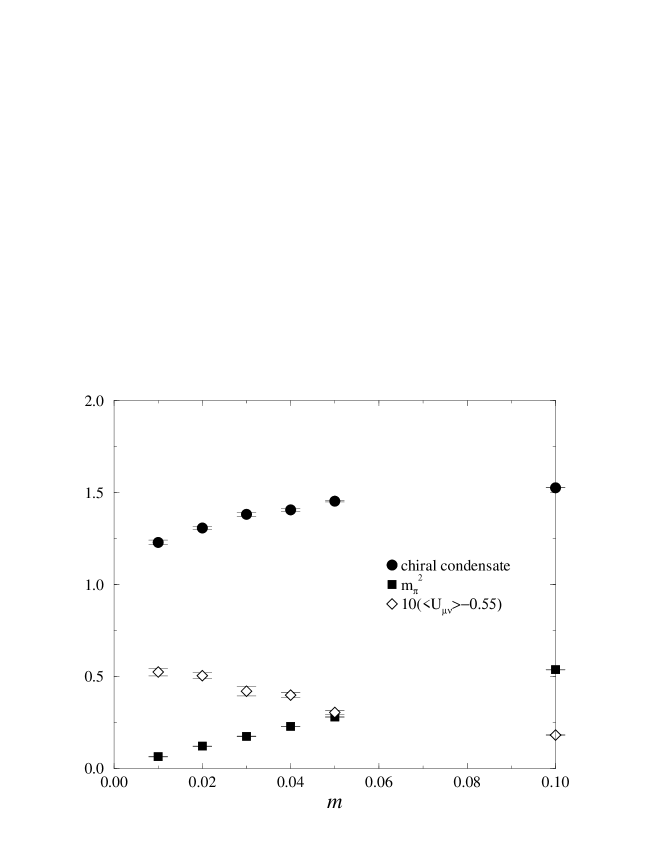
Figure 4: Results of HMC simulations at $\beta=2.0$ on a $4^{3}\times 8$ lattice.

We have performed the bulk of our simulations in this initial study on a $4^{3}\times 8$ lattice with gauge coupling $\beta=2.0$ and quark masses $m=0.1$, 0.05 and 0.01. It is important first to address the issue raised in subsection 2.4, namely whether the model exhibits confinement and chiral symmetry breaking with these parameters at $\mu=0$, or whether the quarks are already sufficiently light to destroy asymptotic freedom and perhaps send the theory into a different phase.

Table 1: Results from simulations with $\mu=0$

$m$	$\langle\bar{\chi}\chi\rangle$	$m_{\pi}$	$\Box$
0.10	1.526(1)	0.7327(4)	0.5682(4)
0.05	1.453(4)	0.5298(16)	0.5805(11)
0.04	1.405(6)	0.4778(14)	0.5899(15)
0.03	1.381(11)	0.4181(15)	0.5921(26)
0.02	1.307(10)	0.3482(18)	0.6004(16)
0.01	1.228(8)	0.2541(25)	0.6033(14)

Fig. 4 shows results obtained by HMC simulation at $\mu=0$ as a function of $m$. The observables monitored, tabulated in Table 1, are the chiral condensate $\langle\bar{\chi}\chi\rangle$ measured using a stochastic estimator, the pion mass $m_{\pi}$ estimated using a standard cosh fit to all 8 timeslices of the pion propagator, and the average plaquette $\Box={1\over 2}\mbox{Tr\,}\langle U_{\mu\nu}\rangle$, which has been rescaled for the convenience of the plot. The data clearly support a scenario with $\lim_{m\to 0}\langle\bar{\chi}\chi(m)\rangle\not=0$ and $m_{\pi}\propto\surd m$ in the same limit. This suggests that simulations with $m\geq 0.01$ fall safely within the regime where chiral symmetry is broken; this suffices for our purposes, since chiral symmetry restoration is the main physical issue at high density. The increase in the value of the plaquette as $m$ is reduced shows nonetheless that color screening due to dynamical fermion effects is clearly observable.

4.2 Autocorrelation Analysis

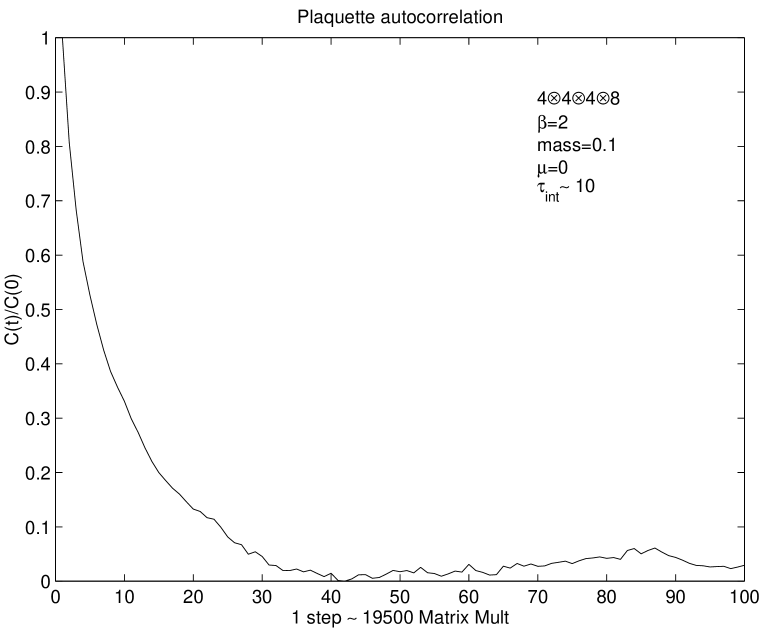
Figure 5: Plaquette autocorrelation function for HMC at $\mu=0.0$

Figure 6: Plaquette autocorrelation function for TSMB at $\mu=0.0$

Before exploring the phase diagram we performed some long runs in order to determine the decorrelation time of both algorithms. A crucial question is how the simulation effort changes for both HMC and TSMB as one follows the $\mu$ axis. To be able to compare two different algorithms we need a common unit of measure for the simulation time necessary to obtain two independent configurations. A convenient choice is the number of matrix multiplications (appropriately corrected with a factor that takes into account that TSMB spends more time in other kinds of operation). For HMC the number of matrix multiplications between two successive data takings is given by:

$$[({{T^{trj}}\over{d\tau}})(I_{cg}^{H})+(I_{cg}^{M})]\times 2\times 2$$ (4.1)

Here $T^{trj}$ is the average trajectory length and $d\tau$ the elementary step length for the hamiltonian deterministic evolution. $I_{cg}^{H}$ is the average number of conjugate gradient iterations for a single step in the hamiltonian evolution, and $I_{cg}^{M}$ is the one needed in the Metropolis selection step. One factor 2 is there because each conjugate gradient iteration implies 2 matrix multiplications, the other because the data are printed out every 2 trajectories.

The corrected number of matrix multiplications to perform a TSMB step is:

$$(n_{2}+n_{3})\times{I_{M}\over 2}\times F$$ (4.2)

Here $I_{M}$ is the number of Metropolis iterations in a single TSMB step and $F$ is the correction factor mentioned above: in practice $F$ is found to depend on every parameter in the simulation, but has typical values $1.2<F<2$.

Since we found the plaquette to be the observable with by far the longest autocorrelation we concentrated on that for the following analysis. First we considered a point at $\mu=0$. The autocorrelation function for a run with HMC is shown in Fig. 5. We deduce an integrated autocorrelation time of the order of $2\times 10^{5}$ matrix multiplications. The corresponding plot for a TSMB run is displayed in Fig. 6. In this case an optimal choice of parameters was found (following the prescription described above) to be $n_{1}=24$, $n_{2}=90$, $n_{3}=110$, $I_{M}=12$. The integrated autocorrelation time turns out to be about $3.2\times 10^{5}$ matrix multiplications.

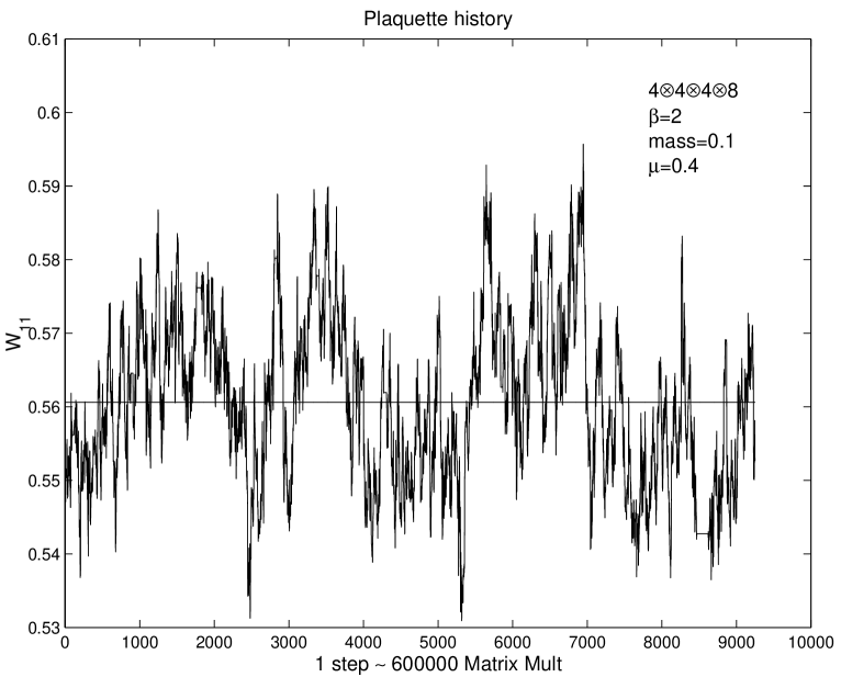
Figure 7: Plaquette time history for HMC at $\mu=0.4$

Figure 8: Plaquette time history for TSMB at $\mu=0.4$

For large values of the chemical potential things get much more difficult for both algorithms. For the representative point at $m=0.1$, $\mu=0.4$ we cannot give a precise determination of the integrated autocorrelations, due to the impracticability of accumulating sufficient statistics. However we can see two typical histories in Figs. 7 and 8. The plots look superficially similar; however one can see from the number of matrix multiplications that the HMC history is much longer, consisting of approximately 15 times more matrix multiplications. This suggests an estimate of the slowing down of HMC with respect to TSMB at that point of about one order of magnitude. The relatively poor performance of HMC in this region arises from the need to reduce $d\tau$ dramatically (values as small as 0.0002 were needed at the highest $\mu$ values explored) to maintain reasonable acceptance. These results strongly suggest that TSMB may be the algorithm of choice in the high density region, independent of the ergodicity considerations discussed in section 3.

Since the integrated autocorrelation time is not available in the high density region, and also because the determinant sign and reweighting factor need to be taken into account, in the following we will quote the jackknife error. For purely gluonic observables such as the plaquette this is probably a considerable underestimate of the true value, and possibly explains why the mean values we present are not really in agreement between the two algorithms. Another factor which may be relevant is the lack of ergodicity of HMC, implying that the two algorithms may be exploring distinct phase spaces; in subsection 4.4 we will show that this is the case for some of the fermionic observables.

4.3 Physics Results from HMC

Next we report on the results of simulations performed using the HMC algorithm for $\mu\not=0$. We used three distinct quark masses on the $4^{3}\times 8$ lattice at $\beta=2.0$, and explored values of $\mu$ up to and including 0.5 for $m=0.1$, $\mu=0.45$ for $m=0.05$, and $\mu=0.3$ for $m=0.01$. Our results for the chiral condensate $\langle\bar{\chi}\chi\rangle$ and the baryon number density $n$ (2.17) are shown as a function of $\mu$ in Fig.  9.

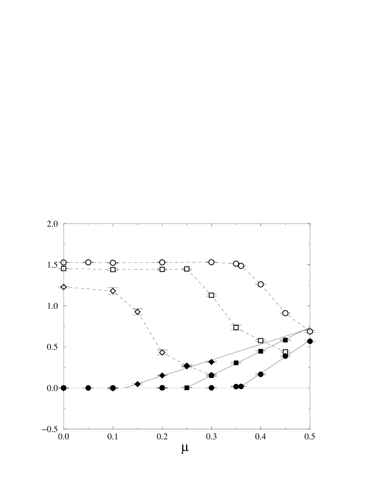
Figure 9: $\langle\bar{\chi}\chi\rangle$ (open symbols) and $n$ (filled symbols) vs. $\mu$, for masses $m=0.1$ (circles), $m=0.05$ (squares) and $m=0.01$ (diamonds).

The results for $m=0.1,0.05$ show the condensates remaining unchanged as $\mu$ increases from zero up to a rather sharply-defined $\mu_{o}$, which we identify with the onset transition discussed in section 2.1. At this point the chiral condensate begins to fall sharply from its zero-density value, and the baryon density begins to rise linearly from zero. The results for $m=0.01$, while less clear-cut, are consistent with this picture. The lines through the filled points are a straight line fit to the non-zero values, the details of which are given in Table 2. The onset value $\mu_{o}$, corresponding to the $x$-intercept of the fit, coincides quite well with the value of $\mu$ for which the edge of the eigenvalue spectrum of $M(\mu)$ crosses the imaginary axis, as illustrated in Fig. 1.

Table 2: Linear fits to $n(\mu)$ in the vicinity of the onset transition

$m$		$x$-Intercept	$x$-Intercept	Slope	Slope
		($\chi$PT)	(measured)	($\chi$PT)	(measured)
0.10		0.3664(2)	0.356(8)	4.548(6)	3.96(6)
0.05		0.2649(8)	0.249(5)	4.141(28)	2.94(4)
0.01		0.1271(13)	0.117(11)	3.044(69)	1.84(8)

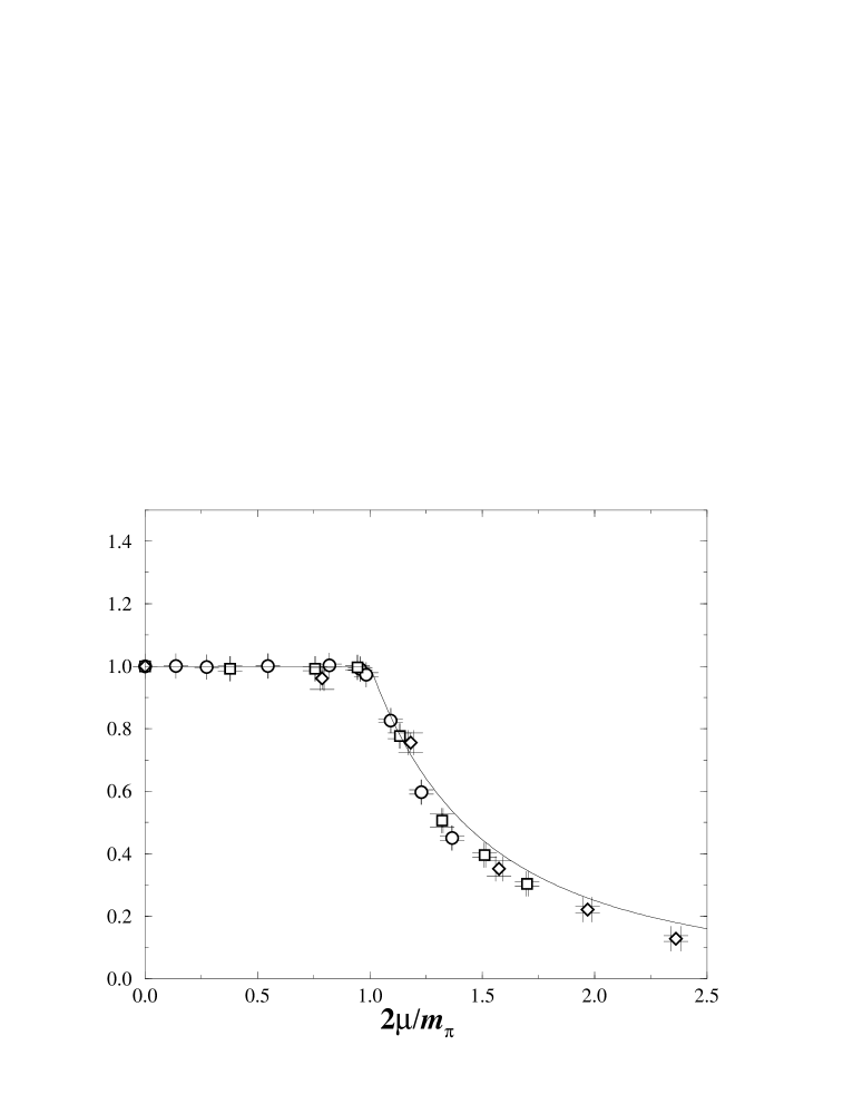
Figure 10: Chiral condensate vs. chemical potential using the rescaled variables of eq. (4.3). The symbols are the same as those of Fig. 9

The picture is qualitatively very similar to the predictions displayed in figure 4 of [9]. We can make the comparison more quantitative by replotting the data in terms of rescaled variables $x=2\mu/m_{\pi 0}$, $y=\langle\bar{\chi}\chi\rangle/\langle\bar{\chi}\chi\rangle_{0}$, and $\tilde{n}=m_{\pi 0}n/8m\langle\bar{\chi}\chi\rangle_{0}$, where the 0 subscript denotes values at zero chemical potential. The predictions from $\chi$PT [9] are then that all data should fall on the lines

$$y=\cases{1&$x<1$,\cr\cr\displaystyle{{1\over x^{2}}}&$x>1$;\cr}\;\;\;\;\;\;\;\;\tilde{n}=\cases{0&$x<1$,\cr\cr\displaystyle{{x\over 4}\left(1-{1\over x^{4}}\right)}&$x>1$.\cr}$$ (4.3)

Using the data of Fig. 9 and Table 1 we plot $y$ vs. $x$ in Fig. 10 and $\tilde{n}$ vs. $x$ in Fig. 11.

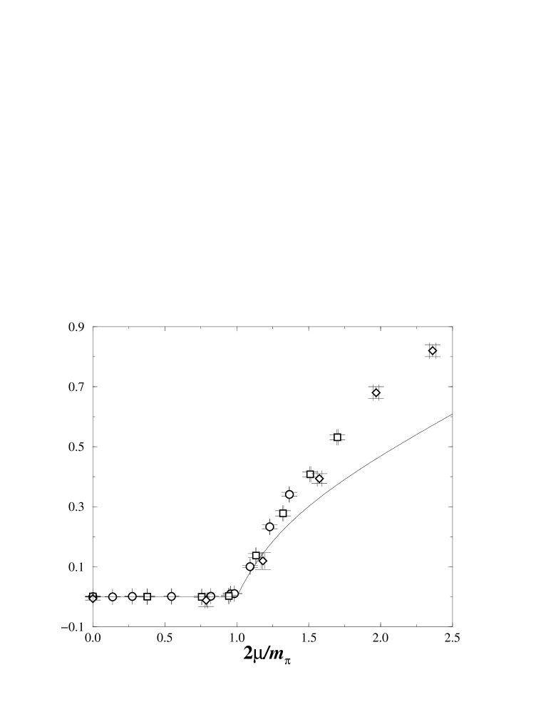
Figure 11: Baryon density vs. chemical potential using the rescaled variables of eq. (4.3).

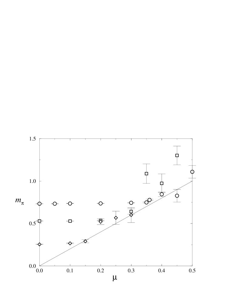
Figure 12: $m_{\pi}$ vs. $\mu$, for masses $m=0.1$ (circles), $m=0.05$ (squares) and $m=0.01$ (diamonds). Also shown is the line $m_{\pi}=2\mu$.

The data collapse very nicely onto a universal curve, corresponding quite closely to the prediction (4.3). The systematic departures from the theoretical curves, downwards for the condensate data and upwards for the baryon density, may well be explicable by higher order corrections in $\chi$PT. In Table 2 we also list $\chi$PT predictions for the slope and $x$-intercept of the linear fit to the baryon density, using a linearised approximation to (4.3):

$$n\simeq 16{{m\langle\bar{\chi}\chi\rangle_{0}}\over m_{\pi 0}^{2}}\left(\mu-{m_{\pi 0}\over 2}\right),$$ (4.4)

The match between theory and measurement is excellent for the intercept and strongly supports the identification $\mu_{o}\simeq m_{\pi}/2$; that for the slope less so. In any case, the agreement between theory and measurement is remarkable for data taken on such a small lattice, relatively far from the continuum limit, with quark masses ranging over an order of magnitude.

It seems reasonable to deduce that the high density phase for $\mu>\mu_{o}$ is superfluid, characterised by a non-zero diquark condensate of the form $qq_{\bf 3}$ (2.19), similar to that observed in lattice simulations of Two Color QCD with fundamental fermions [15]. Work to establish this by direct measurement is in progress. Whilst the quantitative agreement between our results and the theoretical predictions of [9] is gratifying, it also contradicts the symmetry-based arguments of section 2.1 that there are no baryonic Goldstones for $N=1$ staggered flavor, and no gauge-invariant local diquark condensate. We believe that this is because the HMC simulations fail to take into account of the determinant sign (or indeed even to change it) ie. that simulations with functional weight $|\mbox{det}M|$ yield broadly similar results to those with weight $\mbox{det}^{2}M$; the premature onset at $\mu_{o}=m_{\pi}/2$ is therefore a direct manifestation of the sign and/or ergodicity problems.

Next, we investigate $m_{\pi}$ as a function of $\mu$. Recall that for $\mu\not=0$, the pion timeslice propagator is defined as

$$G_{\pi}(t)=\sum_{\vec{x}}M^{-1}_{0,\vec{0}:t,\vec{x}}(\mu)M^{tr-1}_{0,\vec{0};t,\vec{x}}(-\mu),$$ (4.5)

necessitating two inversions of $M$. We implemented (4.5) using a source site and color chosen at random and summing over sink color, performing a simple cosh fit to the resulting $G_{\pi}$ over all 8 timeslices. The fits were stable in the low-density phase, but above the onset transition $G_{\pi}$ became markedly noisier and the fit less convincing, suggesting that perhaps a different functional form is more suitable. Our results for $m_{\pi}$ are shown in Fig. 12. For $\mu<\mu_{o}$ $m_{\pi}$ is constant to quite high precision; for $\mu>\mu_{o}$ it begins to rise. Qualitatively similar behaviour has been observed in the Gross–Neveu model [32]; however in the present case we also have the theoretical treatment of [9], which predicts that in the high density phase the state with the quantum numbers of the pion has mass $m_{\pi}=2\mu$. Whilst the large errors in the dense phase preclude a precise comparison, the clustering of the points just above the line $m_{\pi}=2\mu$ is striking.

The issue of whether chiral symmetry is restored in the dense phase, ie. whether $\lim_{m\to 0}\langle\bar{\chi}\chi(m)\rangle\not=0$, is complicated by the sensitivity of $\mu_{o}$ to $m\propto m_{\pi}^{2}$. Eq. (4.3) suggests that $\langle\bar{\chi}\chi\rangle$ should decrease as $\mu^{-2}$ for $\mu>\mu_{o}$, approaching zero only asymptotically as $\mu\to\infty$. This follows from the idea that the chiral condensate is gradually rotated into a diquark condensate as $\mu$ increases. Fig. 10 shows the first hints of this behaviour. We can, however, take a more pragmatic (as well as more physical) approach and plot $\langle\bar{\chi}\chi(m)\rangle$ at fixed $n$ rather than at fixed $\mu$. This has been done for $n=0.1$ 0.2 and 0.3 using the linear fit to $n(\mu)$ of Table 2 and a simple-minded linear interpolation of the chiral condensate data. The result is shown in Fig. 13.

Figure 13: $\langle\bar{\chi}\chi\rangle$ vs. $m$ for various fixed baryon densities.

Clearly data from more values of $m$ would be needed to make a definitive statement, but there is a suggestion that chiral symmetry is not completely restored, particularly at the lowest density $n=0.1$.

Finally we turn to the effect of the chemical potential on the gauge fields. Since this can only be communicated via fermion loops, any effect we see can be ascribed with certainty to dynamical fermions (we cannot exclude the possibility that all our other observations could have been made for a fraction of the cost in the quenched approximation). Gluonic observables, however, are also much more prone to auto-correlations as described in section 4.2, particularly as the quark mass is reduced. Systematic changes with $\mu$ are therefore quite difficult to observe. In this initial HMC study we have only measured the average plaquette; the results are shown in Fig. 14.

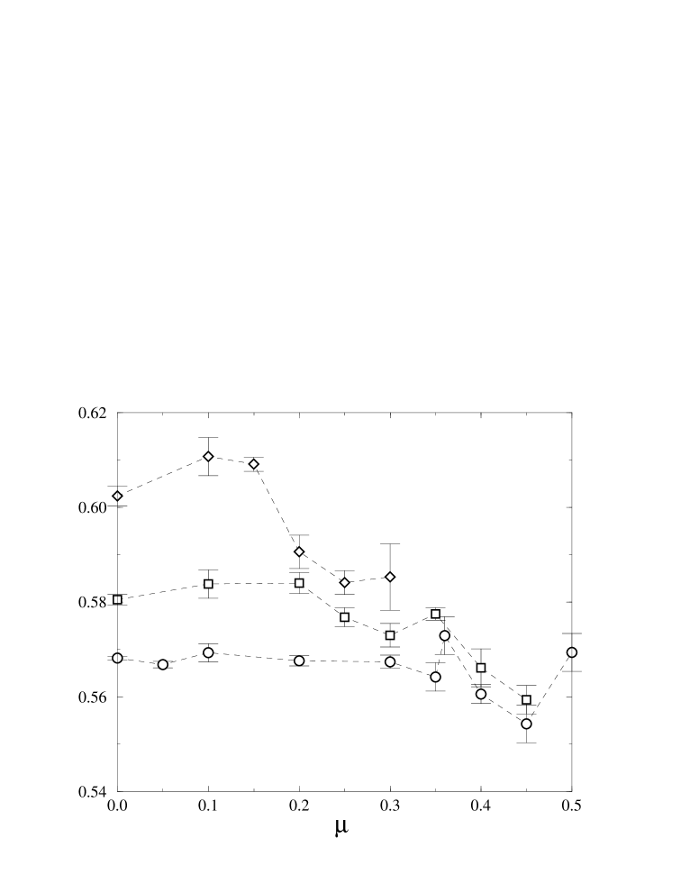
Figure 14: Average plaquette $\Box$ vs. $\mu$ for $m=0.1$ (circles), 0.05 (squares) and 0.01 (diamonds).

The data for $m=0.1$, 0.05 show the plaquette remaining roughly constant for $\mu<\mu_{o}$, before beginning to decrease. The $m=0.01$ data are consistent with this picture within admittedly large errors. We interpret it as follows: for temperature $T=0$, all values of $\mu<\mu_{o}$ are physically equivalent corresponding to the same physical state, namely the vacuum. We only expect an effect on gluonic observables in the presence of matter, ie. for $\mu>\mu_{o}$. To the extent that the results are constant for $\mu<\mu_{o}$ we can be confident that our simulation has an effective $T\simeq 0$. The decrease in the plaquette for $\mu>\mu_{o}$ may be due to the decrease in the number of virtual quark–anti-quark pairs which may form due to the Exclusion Principle — an effect known as Pauli Blocking. This results in a decrease of screening via vacuum polarisation, and hence an effective renormalisation of the gauge coupling $\beta$ and consequent decrease of the plaquette. In the large-$\mu$ limit the lattice should become saturated with one quark of each color per site, and the plaquette assume its quenched value; this has been verified at strong gauge coupling [16].

4.4 Physics Results from TSMB

Each TSMB simulation is characterised by a vector $n_{i}$ specifying the polynomial orders at each stage, as described in section 3.2. For each configuration generated, a reweighting factor $r$ and the sign of $\mbox{det}M$ must be determined. On the relatively small lattices considered here, it is possible to compute $\mbox{det}M$ directly using standard numerical methods; on larger lattices one can use the ‘spectral flow method’ [30] as a function of $m$ and/or $\mu$. The expectation value of an observable $O$ is then determined by the ratio

$$\langle O\rangle={{\langle O\times r\times sign\rangle}\over{\langle r\times sign\rangle}}.$$ (4.6)

Here we present results from runs on a $4^{3}\times 8$ lattice with $\beta=2.0$, $m=0.1$ at three values of chemical potential: $\mu=0.0$ with polynomials $n_{i}=(64,250,300)$; $\mu=0.36$ with both $n_{i}=(64,300,350,500)$ and $n_{i}=(80,300,350,500)$; and $\mu=0.4$ with $n_{i}=(160,1000,1100,1200)$ (reweighting was not performed at $\mu=0.0$). Note that the polynomial orders required increase with $\mu$. The point at $\mu=0$ was chosen to enable the TSMB algorithm to be tested against HMC, since both should yield identical results. The $\mu\not=0$ points were chosen so as to have one value just past the HMC onset transition, where the edge of the eigenvalue distribution just overlaps the line $\mbox{Re}\lambda=0$ and a small percentage of negative determinant configurations are expected, so that hopefully the sign problem is not too severe, and one value fairly deep in the high density phase.

Our results for the standard observables, together with the corresponding HMC results, are summarised in Table 3. For TSMB at $\mu\not=0$ we also include observables determined separately in each sign sector, defined by $\langle O\rangle_{\pm}=\langle O\times r\rangle_{\pm}/\langle r\rangle_{\pm}$. The observables at $\mu=0.36$ and 0.4 result from runs on 32 separate configurations with a few thousand update cycles each. At $\mu=0.0$ the results quoted for $\langle\bar{\chi}\chi\rangle$ and $n$ come from a run on 128 configurations with $\sim$1500 update cycles. Autocorrelation studies reveal that these may not be fully thermalised or decorrelated, which may account for the slight discrepancies between TSMB and HMC. The plaquette at $\mu=0.0$, by far the slowest observable to decorrelate, is taken from a long run of $\sim$25000 update cycles on a single configuration with the same $n_{i}$, with measured autocorrelations taken into account, but ignoring reweighting (reweighting, including $\mbox{sign}(\mbox{det}M)$ has not been observed to have a significant effect on the plaquette). For $\mu=0.0$ and 0.4 the second number quoted results from long runs with 40000 update cycles at $n_{i}=(24,90,120)$ and 19000 at $n_{i}=(140,1000,1100)$ — these runs have been used to obtain Figs. 6 and 8 respectively. Even so, at $\mu=0.4$ the long autocorrelation time implies that the errors are likely to be underestimated, which perhaps explains the large discrepancy between the plaquette value including the measured autocorrelation and the other plaquette values (note also that the HMC plaquette value at $\mu=0.36$ appears to lie outside the trend of Fig. 14).

	$\mu$	TSMB			HMC
		$\langle O\rangle$	$\langle O\rangle_{+}$	$\langle O\rangle_{-}$
$\langle\bar{\chi}\chi\rangle$	0.0	1.510(4)			1.526(1)
	0.36	1.562(18)	1.538(15)	1.240(58)	1.485(9)
	0.4	1.26(15)	1.24(4)	1.23(4)	1.253(10)
$n$	0.0	-0.0018(26)			-0.0002(3)
	0.36	-0.005(14)	0.015(12)	0.263(52)	0.0172(28)
	0.4	0.09(13)	0.17(3)	0.21(3)	0.1667(90)
$\Box$	0.0	0.5765(58)			0.5682(4)
		0.5667(17)
	0.36	0.5541(12)	0.5542(11)	0.5551(18)	0.5729(40)
	0.4	0.588(7)	0.5791(14)	0.5746(15)	0.5612(30)
		0.5523(46)

Table 3: A comparison of results between TSMB and HMC

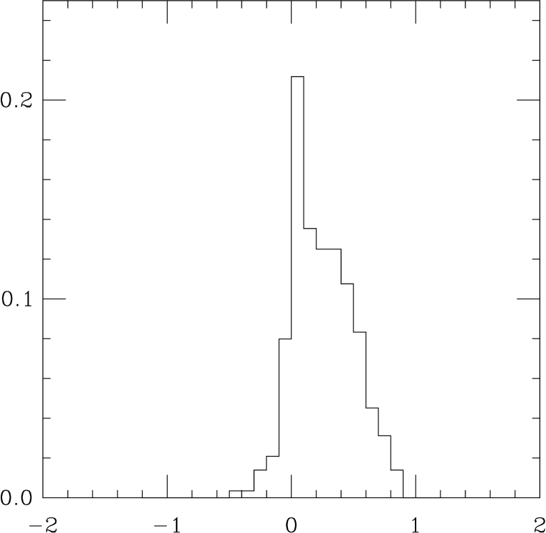
Figure 15: Histogram of $r\times sign$ for $\mu=0.36$ with $n_{i}=(64,300,350,500)$.

Figure 16: Histogram of $r\times sign$ for $\mu=0.40$ with $n_{i}=(200,1000,1100,1200)$.

At $\mu=0.0$ the plaquette results in the second row provide reassurance that the two algorithms agree, and that we have some degree of control over errors. Only once $\mu>\mu_{o}$ (as determined by HMC) do we anticipate the two should differ as a result of HMC’s failure to explore the negative determinant sector. In Figs. 15 and 16 we plot distributions of $r\times sign$ obtained at $\mu=0.36$, 0.4 respectively. For $\mu=0.36$ there is a small fraction of negative determinant configurations; for $\mu=0.4$ the distribution is much more symmetrical between + and –, although the precise shape is found to be sensitive to the choice of $n_{i}$, and $n_{2}$ in particular. The severity of the sign problem in numerical simulations is usually expressed in terms of the average sign $\langle sign\rangle$; generically this decreases towards zero as the system volume increases until its relative error becomes so large that accurate estimates of $\langle O\rangle$ are impracticable. For TSMB the corresponding quantity is not uniquely defined; eg. for the data of Fig. 15 we could specify the fraction of negative determinant configurations (12%), $\langle r\times sign\rangle/\langle r\rangle=0.910$, or $(\langle r\rangle_{+}-\langle r\rangle_{-})/(\langle r\rangle_{+}+\langle r\rangle_{-})=0.491$.

A signal for physical effects associated with the inclusion of the sign of the determinant in the functional measure following (4.6) is that $\langle O\rangle_{+}\not=\langle O\rangle_{-}$. The centre columns of table 3 reveal evidence for such an effect in the fermionic obsevables for $\mu=0.36$. As a result, the full average over both sectors for $\langle\bar{\chi}\chi\rangle$ is significantly greater than the HMC result, and perhaps even consistent with $\langle\bar{\chi}\chi\rangle_{0}$. More spectacularly, the average baryon density $n$ is consistent with zero. These observations imply that at this value of $\mu$ the system is still in the low density phase, and hence $\mu_{o\,TRUE}>\mu_{o\,HMC}$. This is in accord with our symmetry-based arguments that for $N=1$ flavors of adjoint staggered fermion there are no baryonic Goldstones and hence no early onset. Note that similar effects seen at $\mu=0.4$ are statistically far less significant, and should at this stage be considered preliminary.

We have seen that TSMB simulations give evidence for a delayed onset, giving us confidence that the algorithm correctly samples the two sign sectors and thus correctly describes a single flavor. This is the principal result of our initial TSMB studies.

5 Conclusions

To our knowledge this has been the first study of Two Color QCD with adjoint quarks, and the first TSMB study both to use staggered fermions, and to set $\mu\not=0$. The highlights of this work are the following:

• We have outlined the global symmetries and anticpated patterns of symmetry breaking for SU(2) lattice gauge theory with staggered fermions and a non-zero chemical potential in both fundamental and adjoint representations. The case of $N=1$ adjoint flavor seems especially interesting, being the most ‘QCD-like’.

• We have studied the model using both conventional hybrid Monte Carlo (HMC) and Two-Step Multi-Bosonic (TSMB) algorithms. The HMC simulations slow down dramatically, both in terms of number of matrix inversions required, and in terms of autocorrelation, once the eigenvalue distribution includes some with negative real part, which begins to occur once baryon density $n>0$. We have confirmed the existence of isolated real negative eigenvalues at large $\mu$ and hence a sign problem. The HMC algorithm is unable to change the sign of the determinant, and hence is not ergodic in this region. The TSMB algorithm, by reason of the approximate way in which it treats small eigenvalues, is able to change the determinant sign — our first studies also indicate it decorrelates more effectively than HMC in the dense phase.

• Simulations using HMC over a range of $m$ and $\mu$ show good quantitative agreement with a chiral perturbation theory treatment — data spanning an order of magnitude in quark mass collapsing onto a simple universal curve whose parameters are completely determined by physical quantities measured at $\mu=0$. In particular a second order phase transition (see Fig. 11) at $\mu=m_{\pi}/2$ separates the vacuum from a phase with $n>0$, which can be interpreted as a fluid of mutually repelling diquark bosons [9]. The $\chi$PT analysis should only hold for the global symmetries of the model with $N\geq 2$ flavors, implying that the failure to explore the negative determinant sector of the model results in the ‘wrong’ physics.

• Measurements made using TSMB simulations which take the determinant sign into account give evidence for a delayed onset, ie. $n$ remains consistent with zero even for $\mu>m_{\pi}/2$. This is in accord with the symmetry breaking pattern anticipated for $N=1$.

In the future we plan to extend our simulations of the dense phase using both algorithms, with the following goals:

• We wish to examine the spectrum of the model at $\mu=0$ in greater detail, in order to establish the masses of baryonic states such as vector diquarks, $qg$ fermions, etc, which may be associated with further thresholds as they are induced into the ground state as $\mu$ is raised. We expect the $\chi$PT treatment, which does not include such states, to cease to be accurate at some point. This may be signalled either by the breakdown of universality of data with different $m$, or by further phase transitions.

• We wish to probe larger values of $\mu$, up to the saturation point $n\simeq 3$ quarks per lattice site, to see whether any new phases emerge. Perhaps at some point a sharp Fermi surface will appear.

• We wish to explore gluodynamics in the dense medium [10], by studying (in order of sophistication) Pauli Blocking, the static quark potential, the gluon propagator, and the spatial and size distribution of instantons. These studies will require a sizeable increase in lattice volume.

• We wish to explore signals for diquark condensation in the dense phase, both in superfluid and superconducting channels. This latter exotic phenomenon will require good quantitiative control over the determinant sign fluctuations, and hence high statistics (though probably not a large volume).

References

- [1] D. Bailin and A. Love, Phys. Rep. 107 (1984) 325.
-
[2]
M. Alford, K. Rajagopal and F. Wilczek, Phys. Lett. B422
(1998) 247;
R. Rapp, T. Schäfer, E.V. Shuryak and M. Velkovsky, Phys. Rev. Lett. 81 (1998) 53. - [3] M. Alford, K. Rajagopal and F. Wilczek, Nucl. Phys. B537 (1999) 443.
-
[4]
A. Gocksch, Phys. Rev. D37 (1988) 1014, Phys. Rev.
Lett. 61 (1988) 2054;
M.A. Stephanov, Phys. Rev. Lett. 76 (1996) 4472. - [5] I.M. Barbour, S.J. Hands, J.B. Kogut, M.-P. Lombardo and S.E. Morrison, Nucl. Phys. B557 (1999) 339.
- [6] M.E. Peskin, Nucl. Phys. B175 (1980) 197.
-
[7]
E. Dagotto, F. Karsch and A. Moreo, Phys. lett. B169
(1986) 421;
E. Dagotto, A. Moreo and U. Wolff, Phys. Lett. B186 (1987) 395. - [8] S.J. Hands, J.B. Kogut, M.-P. Lombardo and S.E. Morrison, Nucl. Phys. B558 (1999) 327.
- [9] J.B. Kogut, M.A. Stephanov, D. Toublan, J.J.M. Verbaarschot and A. Zhitnitsky, hep-ph/0001171.
- [10] M.-P. Lombardo, hep-lat/9907025.
- [11] M. Lüscher, Nucl. Phys. B 418 (1994) 637.
-
[12]
H. Kluberg-Stern, A. Morel and B. Petersson, Nucl. Phys.
B215 (1983) 527;
J.B. Kogut, H. Matsuoka, M. Stone, H.W. Wyld, S. Shenker, J. Shigemitsu and D.K. Sinclair, Nucl. Phys. B225 (1983) 93;
S.J. Hands and M. Teper, Nucl. Phys. B347 (1990) 819;
J.J.M. Verbaarschot, Phys. Rev. Lett. 72 (1994) 2531. - [13] J.B. Kogut, M.A. Stephanov and D. Toublan, Phys. Lett. B464 (1999) 183.
- [14] S.J. Hands and S.E. Morrison, Phys. Rev. D59:116002 (1999).
- [15] S.E. Morrison and S.J. Hands, proceedings of Strong and Electroweak Matter ’98, Copenhagen, 2nd-5th December 1998, eds. J. Ambjørn et al, p. 364, hep-lat/9902012.
- [16] S.J. Hands and S.E. Morrison, proceedings of Understanding Deconfinement in QCD, ECT∗ Trento, 1st-13th March 1999, eds. D. Blaschke et al, p. 31, hep-lat/9905021.
- [17] H. Georgi and S.L. Glashow, Phys. Rev. Lett. 28 (1972) 1494.
- [18] A. Hart, O. Philipsen, J.D. Stack and M. Teper, Phys. Lett. B396 (1997) 217.
- [19] E. Fradkin and S. Shenker, Phys. Rev. D19 (1979) 3682.
- [20] T. Schäfer and F. Wilczek, Phys. Rev. Lett. 82 (1999) 3956.
- [21] H. Kluberg-Stern, A. Morel, O. Napoly and B. Petersson, Nucl. Phys. B220 [FS8] (1983) 447.
- [22] S. Duane, A.D. Kennedy, B.J. Pendleton and D. Roweth, Phys. Lett. B195 (1987) 216.
- [23] I. Montvay, Nucl. Phys. B 466 (1996) 259.
-
[24]
I.M. Barbour, N. Behilil, E. Dagotto, F. Karsch, A. Moreo, M.
Stone and H.W. Wyld, Nucl. Phys. B275 [FS17] (1986) 296;
C.T.H. Davies and E.G. Klepfish, Phys. Lett. B256 (1991) 68. - [25] M. Halasz, J. Osborn and J. Verbaarschot, Phys. Rev. D56 (1997) 7059.
- [26] S. Chandrasekharan and U.-J. Wiese, Phys. Rev. Lett. 83 (1999) 3116.
-
[27]
S.J. Hands, A. Kocić and J.B. Kogut, Nucl. Phys.
B390 (1993) 355;
J.B. Kogut, M.A. Stephanov and C.G. Strouthos, Phys. Rev. D58 (1998) 096001;
S. Chandrasekharan, J. Cox, K. Holland and U.-J. Wiese, Nucl. Phys. B576 (2000) 481;
J. Cox and K. Holland, hep-lat/0003022 - [28] R. Kirchner, I. Montvay, J. Westphalen, S. Luckmann and K. Spanderen, Phys. Lett. B446 (1999) 209.
-
[29]
I. Montvay, Comput. Phys. Commun.109 (1998) 144;
I. Montvay, talk at Interdisciplinary Workshop on Numerical Challenges in Lattice QCD, Wuppertal, Germany, Aug. 1999, hep-lat/9911014. - [30] I. Campos, R. Kirchner, I. Montvay, J. Westphalen, A. Feo, S. Luckmann, G. Münster and K. Spanderen, Eur. Phys. J. C11 (1999) 507.
- [31] R. Frezzotti and K. Jansen, Phys. Lett. B402 (1997) 328.
- [32] S.J. Hands, S. Kim and J.B. Kogut, Nucl. Phys. B442 (1995) 364.