Physical Results from Unphysical Simulations

Abstract

We calculate various properties of pseudoscalar mesons in partially quenched QCD using chiral perturbation theory through next-to-leading order. Our results can be used to extrapolate to QCD from partially quenched simulations, as long as the latter use three light dynamical quarks. In other words, one can use unphysical simulations to extract physical quantities—in this case the quark masses, meson decay constants, and the Gasser-Leutwyler parameters $L_{4}-L_{8}$. Our proposal for determining $L_{7}$ makes explicit use of an unphysical (yet measurable) effect of partially quenched theories, namely the double-pole that appears in certain two-point correlation functions. Most of our calculations are done for sea quarks having up to three different masses, except for our result for $L_{7}$, which is derived for degenerate sea quarks.

UW/PT 00-10

hep-lat/0006017

I Introduction

A major obstacle to direct simulations of lattice QCD is the difficulty in simulating with light dynamical quarks. In particular, the up and down quarks must be reached by a chiral extrapolation. In present simulations one must do this extrapolation from roughly $m_{s}/2$, where $m_{s}$ is the physical strange quark mass. This is far from the light quark masses ($\overline{m}=(m_{u}+m_{d})/2\approx m_{s}/25$).

The aim of this paper is to provide formulae which can aid in this extrapolation. To do this we use chiral perturbation theory (ChPT) at next-to-leading order (NLO). The parameters of the chiral Lagrangian that enter at this order are the Gasser-Leutwyler (GL) coefficients, $L_{1}-L_{10}$. An alternative way to view the extrapolation to QCD is that, by fitting numerical results in a region where quark masses are considerably larger than the physical light quarks, but small enough that NLO chiral perturbation theory is sufficiently accurate, one determines the relevant $L_{i}$. These are physical parameters of QCD, governing many different physical properties (e.g. pion masses and scattering amplitudes). With the $L_{i}$ in hand, one can then extrapolate to QCD, and, in particular, determine the physical light quark masses. For example, as has been stressed in Refs. [1, 2], determining the combination $2L_{8}-L_{5}$ with only moderate accuracy might allow one to rule out the interesting possibility that $m_{u}=0$. The accuracy of extrapolation depends, of course, on the reliability of NLO chiral perturbation theory. This can be studied by seeing how well the numerical data fit the expected forms, including the curvature predicted by chiral logarithms.

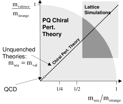
FIG. 1.: Schematic representation of the space of PQ theories for “light” quarks (defined as lighter than the physical strange quark mass). The approximate range of present simulations is shown. The shape of this region is determined by the fact that critical slowing down is less severe for valence quarks than for sea quarks.

An observation of practical importance is that one can make use of partially quenched (PQ) simulations to aid in the extrapolation to QCD [2, 1]. In partially quenched simulations, one changes the mass of the valence quarks (typically reducing them), while holding the dynamical (or “sea”) quark masses fixed. The situation is illustrated schematically in Fig. 1. This leads one into a space of unphysical theories, from which one might expect to obtain only qualitative information about QCD. It turns out, however, that, if all quark masses (valence and sea) are small enough, one can use PQ theories to obtain quantitative information about unquenched theories. Since it is computationally less demanding to reduce valence quark masses, PQ simulations are often used to obtain approximate information on QCD. Our point here is that they can be used to obtain exact information about QCD.

This observation follows from the structure of chiral perturbation theory (ChPT) generalized to partially quenched theories—PQChPT [3]. The key point is that there is a subspace of quark masses (corresponding to the diagonal line in Fig. 1) where PQChPT is completely equivalent to chiral perturbation theory for unquenched, QCD-like theories. Since the quark mass dependence in PQChPT is explicit, as in ChPT, it follows that the parameters of the PQ chiral Lagrangian (with 3 light sea quarks) are the same as those of QCD. These parameters do, however, depend on the number of sea quarks, $N$. This means that PQ simulations with $N=3$ light sea quarks, whatever their precise masses, give information about the parameters of the chiral Lagrangian of QCD. On the other hand PQ simulations with $N=2$ or $N=4$, the values used in most simulations to date, do not give direct information about QCD, even after extrapolation.

These comments motivate the calculation of the NLO chiral corrections to physically interesting quantities in PQ theories. Some results already exist in the literature: those for charged pion masses and decay constants with degenerate sea quarks [4, 5], heavy-light meson properties [8], vector and tensor meson properties [6], baryons masses at large $N_{c}$ [7], and electroweak amplitudes [5]. We provide here two new results. First, charged pion masses and decay constants are considered for non-degenerate sea quarks (having up to three different masses). This completes the calculations of simple pion properties for any theory that is likely to be simulated. It allows one to determine $L_{4-6}$ and $L_{8}$. Note that, although non-degenerate sea quarks are not necessary in order to extract these GL coefficients, as has been stressed in Refs. [1, 2], there is no drawback to using them. Indeed, someone might prefer to extrapolate using more “QCD-like” simulations with two degenerate “light” dynamical quarks and one dynamical quark with mass fixed close to the physical strange quark mass. Our formulae apply for such a theory.

Our second new result concerns the GL coefficient $L_{7}$. In QCD, this contributes only to neutral meson masses, and does so proportional to $(m_{s}-\overline{m})^{2}$. To determine $L_{7}$ using meson masses from unquenched simulations thus requires non-degenerate quarks. At first sight, PQ simulations do not improve the situation: neutral meson masses are still independent of $L_{7}$ when the sea quarks are degenerate. We find, however, that one can determine $L_{7}$ from the coefficient of the double-pole in the propagators of neutral valence mesons, even for degenerate sea quarks. This is a nice example of the utility of PQ theories. Although the double-pole is itself an indicator that these theories are unphysical, its effects can nevertheless be measured in lattice simulations, and its inferred coefficient turns out to be related to a physical quantity.

Throughout our calculations, we treat the $\eta^{\prime}$ as a heavy particle, and integrate it out, following Ref. [4]. This greatly simplifies the resulting expressions, since it removes the dependence on additional $\eta^{\prime}$ coupling constants. It raises, however, two important issues. First, is the $\eta^{\prime}$ heavy enough that removing it is appropriate? The answer depends on the number of light sea quarks, $N$, and the number of colors, $N_{c}$. For the physical values of these parameters, $N=N_{c}=3$, we know from experiment that $M_{\eta^{\prime}}\approx 1\;$GeV. Since this is the scale at which chiral perturbation theory breaks down, it is appropriate to integrate out the $\eta^{\prime}$ for these theories. We stress, however, that our formulae are only valid when the dynamical quarks are light enough that all pseudo-Goldstone bosons, including those composed only of sea quarks, satisfy $M_{PGB}^{2}\ll M_{\eta^{\prime}}^{2}$. For further discussion of this point, and of the limitations of the approach taken here, see Ref. [5].

The second issue is more technical. How does one integrate out the $\eta^{\prime}$ in PQ theories? In this paper we follow Ref. [4] and do this by hand, working only at tree level. This is unsatisfactory, since, as we know from QCD, $\eta^{\prime}$ loops to all orders give contributions of the same order in chiral perturbation theory. In other words, the $\eta^{\prime}$ must be integrated out non-perturbatively. We return to this issue in a companion paper, where we demonstrate that the approach adopted here is equivalent to integrating out the $\eta^{\prime}$ non-perturbatively in the PQ theory [9].

This paper is organized as follows. In the following section we recall the formalism of PQ chiral perturbation theory, and explain our calculational procedure. After presenting a simple form for the neutral meson propagator in Sec. III, we give our results for charged pion properties in Sec. IV. We analyze these results in Sec. V, paying particular attention to the convergence of the chiral expansion and the importance of non-analytic terms. In Sec. VI we explain how to extract $L_{7}$ using PQ theories. We end with some conclusions. Two appendices deal with technical issues in the calculation of the neutral meson propagator.

Some parts of this work have been reported previously in Ref. [2].

II Theoretical framework

We consider partially quenched theories with the following quark complement: $N_{1}+N_{2}+N_{3}=N$ sea quarks, $N_{i}$ each of mass $m_{i}$; two valence quarks with masses $m_{A}$ and $m_{B}$; and two corresponding ghost quarks with masses $m_{\tilde{A}}=m_{A}$ and $m_{\tilde{B}}=m_{B}$. The ghosts are needed to cancel the determinant arising from the valence quark functional integral [10]. In the chiral limit, this theory has an $SU(N+2|2)_{L}\otimes SU(N+2|2)_{R}$ symmetry group [3]. If $N_{1}=N_{2}=N_{3}=1$, and $m_{1}=m_{u}$, $m_{2}=m_{d}$ and $m_{3}=m_{s}$, then the sea-quark sector is QCD. Generalizing to arbitrary numbers $N_{i}$ covers most other theories that are likely to be simulated in an effort to shed light on QCD.

An important property of PQ theories, which follows trivially from their definition, is that the sea-quark sector decouples from the valence sector. To be precise, all correlation functions composed of only sea-quark fields are identical to those in the unquenched sea-quark theory. There is no “back-reaction” from the valence sector. The same result must also hold for the low energy chiral Lagrangian describing the PQ theory: correlators of pseudo-Goldstone mesons composed of sea quarks should be the same as in the chiral Lagrangian describing the unquenched theory. This was shown to be true in Ref. [3]. In practice, however, one might view all correlation functions that are calculated as being those of valence quarks, and so it is more useful to reformulate this property as follows. When each of the valence quarks is assigned a mass that is equal to one of the sea quark masses, sea and valence quarks become indistinguishable, and the cancelations of the “doubled” quark species against their ghost counterparts trivially render the theory the same as an unquenched theory containing only the “original” sea quarks. That this is so was also shown in Ref. [3], and it has important consequences in the following.

At low energies, the partially quenched chiral effective theory is expressed in terms of the fields [3]

$$\Sigma = \exp({2i\Phi}/{f})\,,$$ (1)

$$\Phi = \left(\Phi_{ab}\right)=\frac{1}{\sqrt{2}}\left(\pi_{ab}\right),\ a,b\in\{A,B,1,2,\ldots,N,\tilde{A},\tilde{B}\}\,,$$ (2)

$$\Phi_{0} = \mbox{str}\,\Phi/\sqrt{N}\,,$$ (3)

and the quantity

$$\chi=2\mu m=2\mu\mbox{ diag}(m_{A},m_{B},\underbrace{m_{1},\ldots,m_{1}}_{N_{1}},\underbrace{m_{2},\ldots,m_{2}}_{N_{2}},\underbrace{m_{3},\ldots,m_{3}}_{N_{3}},m_{A},m_{B})\,.$$ (4)

where $m$ is the quark mass matrix. In the following we use the notation $\chi_{A}=2\mu m_{A}$, $\chi_{1}=2\mu m_{1}$, etc. The constants $f$ and $\mu$ are unknown parameters. The fields $\pi_{ab}$ describe the pseudo-Goldstone particles of the theory—we refer to them generically as mesons even though some are fermionic. Because of the anomaly, arbitrary functions of the field $\Phi_{0}$ (the super-$\eta^{\prime}$) can appear in the Lagrangian.

The partially quenched chiral effective Lagrangian is expanded in powers of $\epsilon^{2}\sim M^{2}/\Lambda^{2}\sim p^{2}/\Lambda^{2}$, where $M$ is a typical pseudoscalar meson mass, $p$ the momentum, and $\Lambda\sim 1\;$GeV is the scale beyond which the theory breaks down.

The parts of the Euclidean Lagrangian contributing to meson masses and decay constants at one-loop order are:

$${\mathcal{L}}_{\rm LO} = \frac{f^{2}}{4}\mbox{str}\left(\partial_{\mu}\Sigma\partial_{\mu}\Sigma^{\dagger}\right)-\frac{f^{2}}{4}\mbox{str}\left(\chi\Sigma^{\dagger}+\Sigma\chi\right)+\alpha\partial_{\mu}\Phi_{0}\partial_{\mu}\Phi_{0}+m_{0}^{2}\Phi_{0}^{2}$$ (5)

$${\mathcal{L}}_{\rm NLO,1} = L_{4}\,\mbox{str}\left(\partial_{\mu}\Sigma\partial_{\mu}\Sigma^{\dagger}\right)\mbox{str}\left(\chi\Sigma^{\dagger}+\Sigma\chi\right)+L_{5}\,\mbox{str}\left[\partial_{\mu}\Sigma\partial_{\mu}\Sigma^{\dagger}\left(\chi\Sigma^{\dagger}+\Sigma\chi\right)\right]$$ (7)

$$\mbox{ }-L_{6}\left[\mbox{str}\left(\chi\Sigma^{\dagger}+\Sigma\chi\right)\right]^{2}-L_{8}\,\mbox{str}\left(\chi\Sigma^{\dagger}\chi\Sigma^{\dagger}+\Sigma\chi\Sigma\chi\right)$$

$${\mathcal{L}}_{\rm NLO,2} = -L^{\prime}_{7}\left[\mbox{str}\left(\chi\Sigma^{\dagger}-\Sigma\chi\right)\right]^{2}+v_{1}\Phi_{0}^{2}\mbox{str}\left(\partial_{\mu}\Sigma\partial_{\mu}\Sigma^{\dagger}\right)$$ (9)

$$\mbox{ }+v_{2}\Phi_{0}^{2}\mbox{str}\left(\chi\Sigma^{\dagger}+\Sigma\chi\right)$$

The coefficients $\alpha$, $m_{0}$, $L_{i}$ and $v_{i}$ are further unknown parameters of the low energy theory. The $L_{i}$ depend, in general, on the renormalization scale. The NLO Lagrangian is broken into two parts because flavor off-diagonal mesons receive contributions only from ${\mathcal{L}}_{\rm NL0,1}$.

At this point we can make clear the relationship between the partially quenched chiral Lagrangian and that describing low energy QCD. The latter is obtained by setting $N=3$, and “unquenching” — i.e. assigning $m_{A}$ and $m_{B}$ values from $\{m_{1},m_{2},m_{3}\}$. It follows that the unknown coefficients in ${\mathcal{L}}$ are, for $N=3$, identical to those in the QCD chiral Lagrangian. This shows that these constants also govern the chiral behavior of PQ extensions of QCD.

In QCD, one can take a further step and “integrate out” the $\eta^{\prime}$. This is appropriate since it is not a pseudo-Goldstone boson, having $M_{\eta^{\prime}}^{2}\approx m_{0}^{2}+O(m)\approx 1\;{\rm GeV}^{2}$. Technically, the matching between theories with and without the $\eta^{\prime}$ is non-perturbative, since loops involving the $\eta^{\prime}$ are not suppressed by powers of $M^{2}$ or $p^{2}$. Thus in the standard approach one simply writes down the Lagrangian without the $\eta^{\prime}$, and it has the same form as Eqs. (5)-(9), except that $\Phi$ is traceless. It follows that $\alpha$, $m_{0}$ and the $v_{i}$ are irrelevant, and the only NLO coefficients are the $L_{i}$. It is in fact in this theory that the $L_{i}$—the Gasser-Leutwyler coefficients—are conventionally defined.

In previous work on PQQCD, the step of integrating out the $\eta^{\prime}$ has been done by hand, i.e. at the level of individual diagrams rather than the Lagrangian [4]. We summarize the procedure here—details will become apparent in the following section.

• Loop diagrams involving the $\eta^{\prime}$ are dropped, since these lead to shifts in the parameters $L_{i}$ which are automatically included if we use the $L_{i}$ from the QCD Lagrangian without the $\eta^{\prime}$.

• Couplings special to the $\eta^{\prime}$, such as the $v_{i}$ in Eq. (9), are treated as small, of $O(\epsilon^{2})$, and thus appear only at tree level. The justification for this treatment is that these couplings are suppressed by powers of $1/N_{c}$, in this case $1/N_{c}^{2}$.

• On the other hand, the parameter $m_{0}^{2}$ is treated non-perturbatively since it is known to be $\sim\Lambda^{2}$, despite the fact that it is proportional to $1/N_{c}$. In particular, we treat $M^{2}/m_{0}^{2}$ as $O(\epsilon^{2})$ (with $M$, as above, a typical meson mass). For convenience, we also treat $\alpha$ non-perturbatively.

While this procedure may be accurate enough for phenomenological purposes, it is theoretically unsatisfactory because the $\eta^{\prime}$ should be integrated out non-perturbatively. As noted in the introduction, we will address this concern in a separate paper [9]. In particular, we will argue that the procedure adopted here in fact leads to results that are equivalent to those obtained from integrating out the $\eta^{\prime}$ non-perturbatively.

We close this section by deriving a result needed in Sec. VI. We claimed above that discarding $\eta^{\prime}$ loops allows us to write our results in terms of the standard GL coefficients, i.e. those in an effective Lagrangian without the $\eta^{\prime}$. This is not quite correct. Tree diagrams involving an intermediate $\eta^{\prime}$, which we keep, lead to a shift in $L_{7}$ proportional to $M^{2}/m_{0}^{2}$. Thus we are not using the conventional $L_{7}$, but rather that defined in the effective theory containing the $\eta^{\prime}$, which we denote $L^{\prime}_{7}$ [as anticipated in Eq. (9)]. In order to express our results in terms of conventional parameters, we need to relate $L^{\prime}_{7}$ to $L_{7}$ within the approximations of our procedure.

To determine this relation we need consider only the sea-quark sector, and thus work with the conventional (unquenched) chiral Lagrangian. The $\eta^{\prime}$ field in this theory is the restriction to the sea sector of the “super-$\eta^{\prime}$” field $\Phi_{0}$. To make the $\eta^{\prime}$ dependence explicit, we decompose $\Sigma$ into pseudo-Goldstone and $\eta^{\prime}$ parts:

$$\Sigma=U\exp(\frac{2i\Phi_{0}}{f\sqrt{N}})\,;\qquad U\in SU(N)\,,$$ (10)

and substitute into the chiral Lagrangian. The result is the original form with $\Sigma\to U$ and $\Phi_{0}\to 0$, i.e. the standard QCD chiral Lagrangian, plus the following terms

$${\cal L}_{\Phi_{0}} = c_{1}\Phi_{0}+c_{2}\Phi_{0}^{2}+c_{3}(\partial\Phi_{0})^{2}+O(\Phi_{0}^{3})$$ (11)

$$c_{1} = if\mbox{tr}(\chi U^{\dagger}-\chi U)/(2\sqrt{N})+O(\chi^{2})$$ (12)

$$c_{2} = m_{0}^{2}+O(\chi)$$ (13)

$$c_{3} = 1+\alpha+O(\chi)$$ (14)

Only the leading order terms in the chiral expansion of the coefficients are shown, since higher order terms give contributions to the conventional chiral Lagrangian of orders $\epsilon^{6}$ and higher, too high to effect the matching of the GL coefficients which appear at order $\epsilon^{4}$. For the same reason, the $(\partial\Phi_{0})^{2}$ term can be dropped. Keeping the $\eta^{\prime}$ in tree graphs amounts to doing the functional integral over $\Phi_{0}$ keeping only linear and quadratic terms. The result is a contribution to the conventional chiral Lagrangian of order $\epsilon^{4}$ with the same form as the $L_{7}$ term:

$$-{f^{2}\over 16Nm_{0}^{2}}[\mbox{tr}(\chi U-\chi U^{\dagger})]^{2}(1+O(\chi))\,.$$ (15)

Thus we find, within our approximations, the relation

$$L_{7}=L^{\prime}_{7}-{f^{2}\over 16Nm_{0}^{2}}\,.$$ (16)

III Calculation

Expanding ${\mathcal{L}}_{LO}$ to quadratic order, we obtain the meson propagators. For “charged” mesons (i.e. flavor off-diagonal states) these are

$$G^{C}_{ab}(p)\equiv\int d^{4}xe^{-ip\cdot x}\langle\pi_{ab}(x)\pi_{ba}(0)\rangle={\epsilon_{b}\over p^{2}+(\chi_{a}+\chi_{b})/2}\quad(a\neq b)\,,$$ (17)

where the signature vector is

$$\epsilon_{a}=\left\{\begin{array}[]{cl}1&a\in\{A,B,1,2,3,\dots,N\}\\ -1&a\in\{\tilde{A},\tilde{B}\}\end{array}\right..$$ (20)

The propagators for “neutral” (flavor-diagonal) mesons include the contributions of the super-$\eta^{\prime}$ interactions. A general expression has been given in Ref. [3], but we find it convenient to use an alternative form. The propagator is a matrix acting on the space of neutral meson fields, $\pi_{aa}$, $a=1,N+4$. In app. A we show that

$$G^{N}_{ab} \equiv \int d^{4}xe^{-ip\cdot x}\langle\pi_{aa}(x)\pi_{bb}(0)\rangle$$ (21)

$$= \frac{\epsilon_{a}\delta_{ab}}{p^{2}+\chi_{a}}-\frac{(m_{0}^{2}+\alpha p^{2})/N}{\left(p^{2}+\chi_{a}\right)\left(p^{2}+\chi_{b}\right)}\frac{\left(p^{2}+\chi_{1}\right)\left(p^{2}+\chi_{2}\right)\left(p^{2}+\chi_{3}\right)}{(1+\alpha)\left(p^{2}+M_{\pi_{0}}^{2}\right)\left(p^{2}+M_{\eta}^{2}\right)\left(p^{2}+M_{\eta^{\prime}}^{2}\right)}\;.$$ (22)

Here the ${\pi_{0}}$, $\eta$ and ${\eta^{\prime}}$ are neutral mesons in the sea-quark sector. For $N=3$ they are the usual neutral mesons of QCD; for $N>3$ they are the appropriate generalizations, as explained in the appendix. Their masses are functions of the sea-quark masses, and of the $N_{i}$, as given explicitly in Eqs. (A25)-(A27).

The neutral propagator shows explicitly the unphysical nature of the PQ theory. For example, if $a=b=A$, the second term has a double-pole at $p^{2}=-\chi_{A}$. These double-poles are absent, however, in the physical, sea-quark, sector. This was shown in Ref. [3], but is particularly transparent with our result. For example if $a=b=1$ (or equivalently if $a=b=A$ and $\chi_{A}=\chi_{1}$), then the $(p^{2}+\chi_{1})$ in the numerator reduces the double-pole to a single-pole.

For calculations, it is preferable to rewrite the propagator as a sum of (single or double) poles. For simplicity, we discuss the case when $a\neq b$ and $\chi_{a}\neq\chi_{b}$, for then $G^{N}_{ab}$ has only single poles. For uniformity of notation, we introduce the definitions

$$\chi_{\pi}=M_{\pi_{0}}^{2}\,,\quad\chi_{\eta}=M_{\eta}^{2}\,,\quad\chi_{\eta^{\prime}}=M_{\eta^{\prime}}^{2}\,.\quad$$ (23)

in terms of which

$$G_{ab}^{N} = -\frac{1}{N}\sum_{x=a,b,\pi_{0},\eta,\eta^{\prime}}{R_{x}\over p^{2}+\chi_{x}}\qquad(a\neq b)\,,$$ (24)

$$R_{x} = {(m_{0}^{2}-\alpha\chi_{x})\prod_{i=1,3}(\chi_{i}-\chi_{x})\over(1+\alpha)\prod_{y\neq x}(\chi_{y}-\chi_{x})}\,,$$ (25)

where $x$ and $y$ run over $a,b,\pi,\eta,\eta^{\prime}$. The degenerate limit $\chi_{a}=\chi_{b}$ or $a=b$, which, in general, has double poles is straightforward to obtain.

At this point we are in a position to integrate out the $\eta^{\prime}$ by hand, bearing in mind that this propagator appears in loops. First, as discussed above, we drop the $\eta^{\prime}$ pole. Second, we expand the residues of the remaining poles in powers of $\chi_{x}/m_{0}^{2}$, $x\neq\eta^{\prime}$, and drop all but the leading term. This is justified since we use the neutral propagator in one-loop diagrams, which already give NLO contributions. The only exception is in our discussion of $L_{7}$ in Sec. VI, where the neutral propagator appears at tree-level. With these changes, the residues become

$$R_{x}={\prod_{i=1,3}(\chi_{i}-\chi_{x})\over\prod_{y=a,b,\pi,\eta\atop y\neq x}(\chi_{y}-\chi_{x})}\,.$$ (26)

Note that both $m_{0}^{2}$ and $\alpha$ disappear from the neutral propagator.

IV NLO results

In this section we calculate the properties of a meson composed of two valence quarks to NLO. We use dimensional regularization, and subtract the poles following the conventions of Ref. [12].

Its mass, $M_{AB}$, is obtained from the diagrams of Fig. 2. We find

$$M_{AB}^{2} = \frac{\chi_{A}+\chi_{B}}{2}\left(1+\delta^{M}_{\rm tree}+\delta^{M}_{\rm loop}\right)$$ (27)

$$\delta^{M}_{\rm tree} = \frac{8N}{f^{2}}\left(2L_{6}-L_{4}\right)\bar{\chi}+\frac{4}{f^{2}}\left(2L_{8}-L_{5}\right)(\chi_{A}+\chi_{B})$$ (28)

$$\delta^{M}_{\rm loop} = \frac{1}{16f^{2}\pi^{2}N}\left\{R_{A}\chi_{A}\log\chi_{A}+R_{B}\chi_{B}\log\chi_{B}+R_{\pi}\chi_{\pi}\log\chi_{\pi}+R_{\eta}\chi_{\eta}\log\chi_{\eta}\right\}$$ (29)

Here $\bar{\chi}$ is the average sea-quark mass,

$$\bar{\chi}=\frac{1}{N}\sum_{i=1,3}N_{i}\chi_{i}\,,$$ (30)

and the residues are defined in Eq. (26). For concreteness we quote two explicit examples

$$R_{A} = \frac{\left(\chi_{A}-\chi_{1}\right)\left(\chi_{A}-\chi_{2}\right)\left(\chi_{A}-\chi_{3}\right)}{\left(\chi_{A}-\chi_{B}\right)\left(\chi_{A}-\chi_{\pi}\right)\left(\chi_{A}-\chi_{\eta}\right)}\,,$$ (31)

$$R_{\pi} = \frac{\left(\chi_{\pi}-\chi_{1}\right)\left(\chi_{\pi}-\chi_{2}\right)\left(\chi_{\pi}-\chi_{3}\right)}{\left(\chi_{\pi}-\chi_{A}\right)\left(\chi_{\pi}-\chi_{B}\right)\left(\chi_{\pi}-\chi_{\eta}\right)}\,.$$ (32)

$R_{B}$ is obtained from $R_{A}$ by interchanging $A$ and $B$, and $R_{\eta}$ is obtained from $R_{\pi}$ by interchanging $\pi$ and $\eta$.

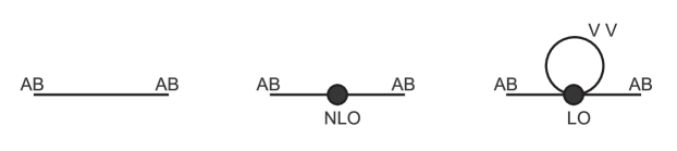
FIG. 2.: Diagrams contributing to $M_{AB}$. The letters next to the lines denote the flavor indices of the propagating mesons. “VV” stands for Valence-Valence meson with $V=A,B$. “LO” and “NLO” describe the order of the vertex that makes the diagram contribute at 1 loop.

The renormalization scale is implicit in the logarithms and the $L_{i}$. Using the result

$$\sum_{x=A,B,\pi,\eta}\chi_{x}R_{x}=(\chi_{A}+\chi_{B}-\bar{\chi})+O(\chi^{2}/m_{0}^{2})$$ (33)

we see that a change in renormalization scale can be absorbed by shifting the $L_{i}$. We have checked (for $N=3$) that the scale dependence of the $L_{i}$ in QCD does render $M^{2}_{AB}$ independent of the renormalization scale.

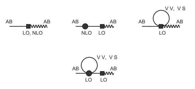
FIG. 3.: diagrams contributing to $f_{AB}$. The wavy line represents the insertion of the axial current operator $j_{5AB}^{\mu}(p)$. “VS” stands for Valence-Sea mesons with $V=A,B$ and $S=1,2,3$.

To determine the meson decay constant, $f_{AB}$, the axial current $j_{5AB}^{\mu}$ is calculated to NLO, and then we evaluate the matrix element

$$\left<0|j_{5AB}^{\mu}|\pi_{AB}(p)\right>=i\sqrt{2}f_{AB}\,p^{\mu},$$ (34)

using the diagrams of Fig. 3. The result is

$$f_{AB} = f\left(1+\delta^{f}_{\rm tree}+\delta^{f}_{\rm VS\ loop}+\delta^{f}_{\rm VV\ loop}\right)$$ (35)

$$\delta^{f}_{\rm tree} = \frac{4N}{f^{2}}\bar{\chi}L_{4}+\frac{2}{f^{2}}(\chi_{A}+\chi_{B})L_{5}$$ (36)

$$\delta^{f}_{\rm VS\ loop} = -\sum_{i=1,3}N_{i}\frac{1}{16\pi^{2}f^{2}}\frac{\chi_{A}+\chi_{i}}{8}\log\left({\chi_{A}+\chi_{i}\over 2}\right)\ +\ \left(A\leftrightarrow B\right)$$ (37)

$$\delta^{f}_{\rm VV\ loop} = \frac{1}{4N}\frac{1}{16\pi^{2}f^{2}}\left\{-D_{A}-D_{B}\right.$$ (40)

$$+{\log(\chi_{A}/\chi_{B})\over(\chi_{A}-\chi_{B})}\left[\chi_{A}D_{A}+\chi_{B}D_{B}+(\chi_{A}-\chi_{B})^{2}\right]$$

$$\left.+\left(\chi_{\pi}R_{\pi}(\chi_{B}\!-\!\chi_{A})\left[{\log(\chi_{\pi}/\chi_{A})\over\chi_{A}-\chi_{\pi}}-{\log(\chi_{\pi}/\chi_{B})\over\chi_{B}-\chi_{\pi}}\right]+\left(\pi\leftrightarrow\eta\right)\right)\right\}$$

where

$$D_{A}={\prod_{i=1,3}(\chi_{i}-\chi_{A})\over(\chi_{\pi}-\chi_{A})(\chi_{\eta}-\chi_{A})}\,,$$ (41)

and $D_{B}$ obtained by $\left(A\leftrightarrow B\right)$, are the coefficients of the double poles in the neutral propagators. It is straightforward to see that the scale dependence can be absorbed by shifts in $L_{4}$ and $L_{5}$, and we have checked that these shifts are consistent with standard results for $N=3$.

As noted in the introduction, our formulae can be used to extract the GL coefficients by fitting to results from simulations. PQ simulations allow one to vary the valence and sea-quark masses independently, and thus to separately determine $L_{4-6}$ and $L_{8}$. In fact, since the NLO analytic terms, Eqs. (28) and (36), depend on the quark masses only through the combinations $\chi_{A}+\chi_{B}$ and $\bar{\chi}$, one need only consider degenerate sea quarks. Indeed, to extract $2L_{8}-L_{5}$, the combination which determines whether $m_{u}=0$, it is sufficient to use a single sea quark mass (as long as it is light enough that the formulae apply), and vary the valence quark masses. By contrast, with unquenched simulations, one would have to use non-degenerate sea quarks to separately determine all four $L$’s.

The most likely practical applications of these results are for simulations done with 2 rather than 3 types of nondegenerate sea quarks. For QCD this would correspond to the limit of exact isospin symmetry. The results for this case can be obtained from those given above by carefully taking the limit $\chi_{2}\to\chi_{1}$. When two types of quark are degenerate, one of the neutral sea-quark eigenstates becomes an exact flavor non-singlet, and we choose this to be the pion. Thus we have $\chi_{\pi}=\chi_{1}=\chi_{2}$. The remaining neutral state has mass $\chi_{\eta}=\chi_{1}+\chi_{3}-\bar{\chi}$. In this limit, the residues simplify, e.g.

$$R_{A} \longrightarrow \frac{\left(\chi_{A}-\chi_{1}\right)\left(\chi_{A}-\chi_{3}\right)}{\left(\chi_{A}-\chi_{B}\right)\left(\chi_{A}-\chi_{\eta}\right)}$$ (42)

$$R_{\pi} \longrightarrow 0$$ (43)

$$R_{\eta} \longrightarrow \frac{\left(\chi_{\eta}-\chi_{1}\right)\left(\chi_{\eta}-\chi_{3}\right)}{\left(\chi_{\eta}-\chi_{A}\right)\left(\chi_{\eta}-\chi_{B}\right)}$$ (44)

with a similar cancelation in the $D_{A,B}$. With these changes, the formulae given above still hold.

We have checked our results in two ways. First, if we take all sea quarks to be degenerate, we obtain the results of Ref. [4]. Second, we can consider the unquenched limit. By choosing $\chi_{A}$ and $\chi_{B}$ to be equal to combinations of $\chi_{1-3}$ we obtain the correct one-loop form for the masses of the $\pi^{+}$, $K^{+}$ and $K^{0}$.

The residues $R_{x}$ and $D_{x}$ are singular when pairs of the $\chi$’s become degenerate, e.g. $\chi_{A}\to\chi_{B}$ and $\chi_{A}\to\chi_{\pi}$. As expected, however, these singularities cancel in the full expressions for $M_{AB}$ and $f_{AB}$, which are analytic functions of the quark masses except in the massless limit.

In Ref. [4], it was emphasized that the one-loop corrections can diverge when the valence-quark masses are sent to zero at fixed sea-quark mass, leading to a breakdown of chiral perturbation theory. This discussion was based on the results for degenerate sea quarks, and we can now generalize it to non-degenerate sea-quarks. For the meson masses, the possibly divergent contribution is $\delta^{M}_{\rm loop}$, and we see that this only diverges if both $m_{A}$ and $m_{B}$ vanish, in fixed ratio, but not if only one vanishes. For the decay constant the pattern is opposite: $\delta^{f}_{\rm VV\ loop}$ diverges if one of the valence masses vanishes, but not if both do in fixed ratio. This is the same pattern of divergences as for degenerate sea quarks; the sea quark masses only influence the coefficients of the divergent $\log\chi_{A}$ and $\log\chi_{B}$ terms. In the following section we discuss the practical implications of these divergences.

It was also noted in Ref. [4] that one can form combinations of the squared meson masses and decay constants from which the analytic correction terms ($\delta_{\rm tree}$) cancel. One thus predicts these combinations in terms of the quark masses and the leading order chiral coefficients $\mu$ and $f$, up to NNLO corrections. Studying these combinations in simulations allows one to test the applicability of NLO chiral perturbation theory. What we want to point out here is that exactly the same quantities can be used for non-degenerate sea-quarks: the $L_{i}$ still cancel. We do not, however, give the explicit expressions since they are lengthy and unilluminating.

Finally, we discuss to what extent our formulae can be applied to lattice results obtained at non-zero lattice spacing. For definiteness, we first consider a calculation using Wilson fermions, in which we work at a fixed bare coupling and vary the bare valence and sea quark masses. Meson properties are of course calculated in lattice units, i.e. we obtain $M_{\pi}a$ and $f_{\pi}a$.

There are two effects of working at a non-zero lattice spacing. The first is that chiral symmetry, upon which our calculation is based, is broken explicitly. This symmetry breaking can, however, be incorporated into the chiral Lagrangian framework, as shown in Ref. [13]. The result is that all effects of the explicit symmetry breaking are of $O(a)$, except for the additive renormalization of the quark masses. Because of this, our formulae are valid, up to corrections of $O(a)$, as long as one uses so-called vector or axial Ward identity quark masses.

Note that the corrections of $O(a)$ cannot be incorporated into our formulae by simply introducing $a$ dependence into the parameters of the chiral Lagrangian parameters, $f$, $\mu$ and the $L_{i}$. There are additional unknown constants which enter.

The second effect is that the lattice spacing itself depends on the quark masses, at fixed bare coupling. This introduces an additional mass dependence into quantities expressed in lattice units. We note, however, that the mass dependence of $a$ is a discretization effect of $O(am)$ induced by the explicit chiral symmetry breaking [14]. Indeed, for non-perturbatively on-shell-improved Wilson fermions one can calculate this dependence, with the result

$$a(m)=a(m\!=\!0)[1-c\,a\overline{m}+\dots]\,,\qquad c={g\ b_{g}(g)\over 2\beta_{\rm LAT}(g)}\,,$$ (45)

where $\overline{m}$ is the average sea-quark mass, $b_{g}(g)\propto g^{2}+O(g^{4})$ is an improvement coefficient introduced in Ref. [14], and $\beta_{\rm LAT}=-dg/d\ln a\propto g^{3}+O(g^{5})$ is the lattice $\beta$-function. Note that this $O(a)$ effect can be absorbed by shifting the GL coefficients as follows:

$$L_{4,6}\rightarrow L_{4,6}-{caf^{2}\over 8N\mu}\,.$$ (46)

Alternatively, one could adjust the bare coupling as the quark masses are varied so as to keep the lattice spacing fixed.

In summary, our formulae are approximately valid for meson properties expressed in lattice units, with the errors being of $O(a)$. Some, but not all, of these discretization errors can be absorbed into $a$ dependence of the parameters of the chiral Lagrangian. With staggered or overlap fermions the errors would instead be of $O(a^{2})$. Since discretization errors can still be substantial at present lattice spacings, it may be better to extrapolate first to $a=0$, and then fit to the predicted forms.

V Behavior of the Chiral Expansion

In the framework of chiral perturbation theory (regardless of quenching) one assumes that for any quantity calculated to a given order in the chiral expansion, higher order terms are smaller. Once the unknown couplings and parameters of the theory are determined (e.g. by experiment, or by fitting to lattice data) the consistency of the computation can be checked numerically. This is the main purpose of the current section.

We can make this check because, using experimental data, we have reasonable estimates for the actual values of some of the Gasser-Leutwyler coefficients. Thus we can use our results to predict the meson masses and decay constants in PQ simulations. Of course, these predictions are approximate because we only know the $L_{i}$ approximately—this is where the lattice results themselves come in—but they give us a reasonable idea of how the chiral expansion behaves.

We consider QCD with exact isospin symmetry, i.e. $N_{1}=N_{2}=N_{3}=1$ and $m_{1}=m_{2}=m_{u}$ and $m_{3}=m_{s}$. The meson masses and decay constants then depend on the seven parameters $f$, $\chi_{u}$, $\chi_{s}$, $L_{4-6}$ and $L_{8}$. We want to choose these parameters so that the four charged meson quantities $M_{\pi}$, $M_{K}$, $f_{\pi}$ and $f_{K}$ take their experimental values. In order to match the number of parameters and observables, we take as starting values the GL coefficients quoted in Ref. [12]. These are based on experimental results ($L_{5}(M_{\eta})\approx 2.3\ 10^{-3},\ L_{8}(M_{\eta})\approx 1.2\ 10^{-3}$) and the large $N_{c}$ limit ($L_{4}(M_{\eta})\approx L_{6}(M_{\eta})\approx 0$). We then take our four free parameters to be $f$, $\chi_{u}$, $\chi_{s}$ and the scale, $\Lambda_{L}$, at which $L_{i}$ take the values just quoted. In effect, this moves us through the space of $L_{i}$ on a particular path, which, when $\Lambda_{L}\approx M_{\eta}$, is consistent with our knowledge about the $L_{i}$. We claim no fundamental basis for this path—we use it for simplicity. It allows us to determine the dimensionless quantities $f/\Lambda_{L}$, $\chi_{u}/f^{2}$ and $\chi_{s}/f^{2}$ by fitting the ratios $M_{\pi}/f_{K},\ M_{K}/f_{K}$ and $f_{K}/f_{\pi}$, and then to determine $\Lambda_{L}$ by requiring, say, $M_{\pi}=140\;$MeV. We find $\Lambda_{L}=M_{\eta}(1-.0021)$ (using $M_{\eta}=547\;$MeV), so that the fitted $L_{i}$’s are, in fact, close to the inputs. The other outputs are $f=85$MeV, $\chi_{u}/\chi_{s}=0.044$ and $\chi_{s}=(673\mbox{MeV})^{2}$.

We stress that we are not claiming that we have found a unique set of parameters. There is a region in the space of the $L_{i}$ which can describe the experimental observables, and for which it turns out that the chiral expansion is under reasonable control. We have picked, somewhat arbitrarily, one point in this region.

We can now explore the behavior of the chiral expansion as a function of the four quantities

$$\left({\chi_{A}\over\chi_{s}},\,{\chi_{B}\over\chi_{s}},\,{\chi_{1}\over\chi_{s}},\,{\chi_{3}\over\chi_{s}}\right)\,.$$ (47)

We have chosen to normalize the various quark masses relative to the physical strange quark mass, so that a ratio of unity represents the outer limit of where one would expect chiral perturbation theory to be reliable. We consider two types of two-dimensional cross-section of the parameter space: $(y,y,x,1)$ and $(y,1,x,1)$. In both cases $y$ corresponds to a valence mass while $x$ is proportional to a sea quark mass. We name these cross-sections the “$\pi$-plane” and the “$K$-plane” because the unquenched line $y=x$ in the former describes a pion-like meson made up of two identical light quarks, whereas, in the latter, $y=x$ corresponds to a kaon-like meson.

We examine the relative size of the NLO contributions by plotting

$$(M_{AB}^{2})_{\mbox{NLO}}/(M_{AB}^{2})_{\mbox{LO}}=(\delta^{M}_{\rm tree}+\delta^{M}_{\rm loop})\equiv\delta^{M}$$ (48)

and

$$(f_{AB})_{\mbox{NLO}}/(f_{AB})_{\mbox{LO}}=\delta^{f}_{\rm tree}+\delta^{f}_{\rm VS\ loop}+\delta^{f}_{\rm VV\ loop}\equiv\delta^{f}$$ (49)

[see Eqs. (27), (35)]. In each plane, these functions are plotted along rays emerging from the origin at angles $15^{\circ},\ 30^{\circ},\ 45^{\circ},\ 60^{\circ}$ and $75^{\circ}$ with respect to the $x$-axis, confined to the unit square (Fig. 4). The $45^{\circ}$ line corresponds to unquenched theories, the other lines to PQ theories. The plots are shown in Figs. 5-8. We also show a contour plot of $\delta^{f}$ in the K-plane in Fig. 9.

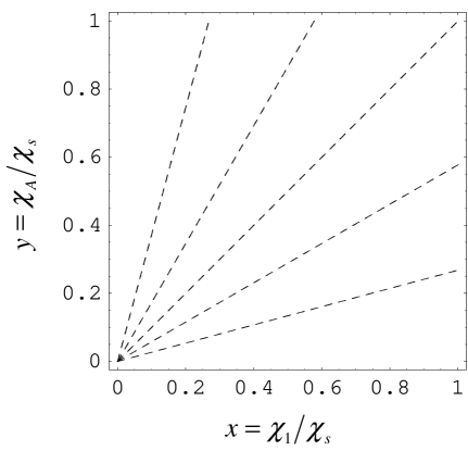
FIG. 4.: The dashed lines are rays in the $\pi$-plane or $K$-plane along which $\delta^{f}$ and $\delta^{M}$ are plotted in Figs. 5-8.

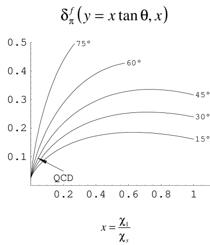
FIG. 5.: $\delta^{f}$ in the $\pi$-plane, $(y,y,x,1)$, is plotted along rays of angle $\theta$ with respect to the $x$-axis (see Fig. 4). The values of theta in degrees are indicated next to the corresponding curves. The point that corresponds to the “physical” pion, $(\chi_{u},\chi_{u},\chi_{u},\chi_{s})$ is labeled “QCD”.

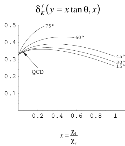
FIG. 6.: Plots of $\delta^{f}$ in the $K$-plane.

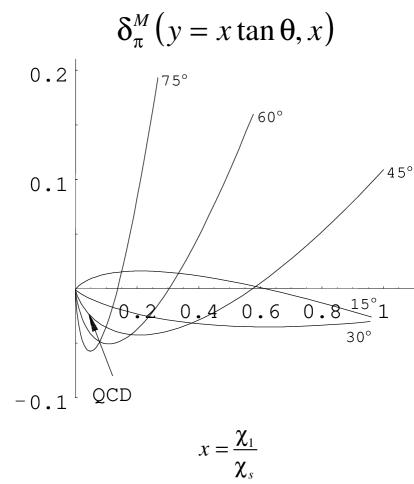
FIG. 7.: Plots of $\delta^{M}$ in the $\pi$-plane.

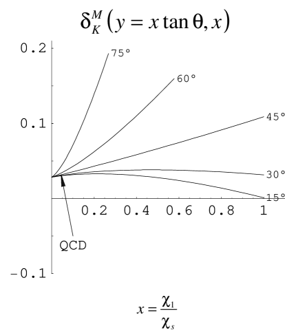
FIG. 8.: Plots of $\delta^{M}$ in the $K$-plane.

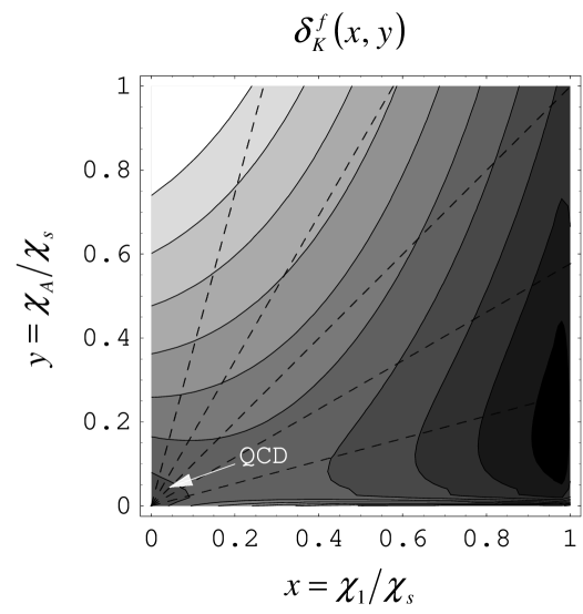
FIG. 9.: Contours of $\delta^{f}_{K}$. The values of $\delta^{f}_{K}$ range from $<.275$ in the black region on the right up to values $>.5$ in the white region. There is a difference of .025 between the values of $\delta^{f}_{K}$ on adjacent contours

The first conclusion that can be drawn from these figures is that chiral perturbation theory for QCD to one-loop order is reasonably convergent throughout the PQ region defined by $\chi_{x}<\chi_{s}$, $x=A,B,1,3$. With our parameters, the least convergent quantity is $f_{K}$. We also note that, generally speaking, the expansion is better behaved when one increases the masses along the lines at small angles. In other words, the expansion may be more reliable when valence masses are smaller than sea-quark masses, and vica-versa. This is good news for simulations, since pushing to small valence quark masses is relatively cheap.

Of course, as noted in the previous section, the valence quark masses cannot be pushed too low at fixed sea masses. At some point the corrections $\delta^{M}$ (in the $\pi$-plane) and $\delta^{f}$ (in the K-plane) diverge. This is not apparent, however, from Fig. 9. To observe the divergence we show in Fig. 10 the region close to the $x$-axis, which does reveal the expected features. Though of theoretical interest, it seems that the breakdown of the chiral expansion due to enhanced chiral logarithms occurs only in a tiny region of parameter space and is therefore of little or no practical significance.

Our final comment concerns the importance of including the non-analytic terms in fits to PQ data. The tree level contributions alone would have produced only straight lines in Figs. 5-8. The curvature seen in the graphs is due to the logarithms originating in loop diagrams. An attempt to model data collected in the heavy quark mass region with only the tree level terms will clearly lead to a significant systematic errors in the extrapolations to QCD values.

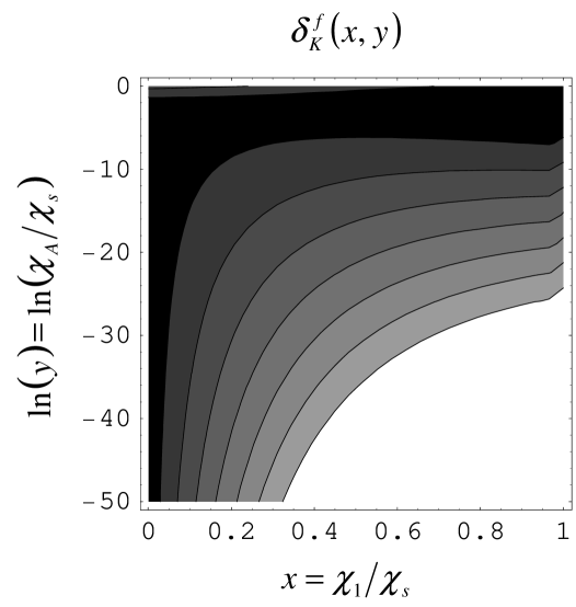
FIG. 10.: Breakdown of the chiral expansion for small values of valence quark mass and a fixed sea quark mass. In the white region, the expansion breaks down as the NLO term in the expression for $f_{K}$ becomes greater than the LO term ($\delta^{f}_{K}>1$). The following contours mark changes of .1 in $\delta^{f}_{K}$, so that the darkest region corresponds to $\delta^{f}_{K}<.4$

VI Determining $L_{7}$

As noted above, the GL coefficients $L_{4}$, $L_{5}$, $L_{6}$ and $L_{8}$ can be obtained using PQ simulations with degenerate sea quarks. Simulations with non-degenerate sea quarks are useful but not essential. In this section we consider the other coefficient which enters into the NLO expressions for the physical meson masses, namely $L_{7}$. This contributes only to flavor-diagonal mesons, i.e. the $\eta$ and $\pi_{0}$ in QCD. Since the contribution is proportional to quark mass differences, the largest effect is on the ${\eta}$ mass. This is conveniently isolated using the violation of the mesonic Gell Mann–Okubo relation [12]

$$4m_{K}^{2}-m_{\pi}^{2}-3m_{\eta}^{2} = {8\over f^{2}}{4(m_{K}^{2}-m_{\pi}^{2})^{2}\over 3}(L_{5}-6L_{8}-12L_{7})$$ (51)

$$\mbox{}+{\left[3m_{\eta}^{4}\log(m_{\eta}^{2})-m_{\pi}^{4}\log(m_{\pi}^{2})-4m_{K}^{4}\log(m_{K}^{2})\right]\over 16\pi^{2}f^{2}}\,.$$

Here we have given the result in the isospin-symmetric limit, i.e. with two degenerate quarks of mass $\overline{m}=(m_{u}+m_{d})/2$, and a single strange quark.

Thus one method for determining $L_{7}$ is to calculate $m_{\eta}$, $m_{K}$ and $m_{\pi}$ in unquenched simulations with non-degenerate sea quarks and fit to the result in Eq. (51). In this section we show how one can obtain $L_{7}$ using degenerate sea quarks by taking advantage of PQ simulations.

A clue on how to proceed is provided by the fact that the ${\eta}$ propagator contains contractions in which the quark propagators are disconnected (“hairpin” contractions). Close to the degenerate limit, these contractions are proportional to $(m_{s}-\overline{m})^{2}$, due to cancelations between light and strange quark propagators. Comparing to Eq. (51), and noting that $m_{K}^{2}-m_{\pi}^{2}\propto m_{s}-\overline{m}$, it is plausible that the $L_{7}$ contribution is related to the disconnected contraction, and that by studying this contraction in the PQ theory one can determine $L_{7}$. This is indeed what we find.

First, we recall the general form of the tree level propagators. In section III we showed that the propagators for flavor off-diagonal mesons, $G_{ab}^{C}$, have an ordinary single pole at the meson mass [Eq. (17)], while $G_{ab}^{N}$, the “neutral” or flavor-diagonal propagators, have a double pole at the same mass if $a=b$ or $m_{a}=m_{b}$ [Eq. (22)]. As we show below, these general forms prevail also at NLO:

$$G_{AB}^{C}(p)\big{|}_{m_{A}=m_{B}} = {{\cal Z_{A}}\over p^{2}+M_{AA}^{2}}+\mbox{non-pole}\,,$$ (52)

$$G_{AB}^{N}(p)\big{|}_{m_{A}=m_{B}} = {{\cal Z_{A}}{\cal D}\over(p^{2}+M_{AA}^{2})^{2}}+\mbox{single-pole}+\mbox{non-pole}\,,$$ (53)

$$G_{AA}^{N}(p) = G_{AB}^{N}(p)\big{|}_{m_{A}=m_{B}}+G_{AB}^{C}\big{|}_{m_{A}=m_{B}}$$ (54)

$$= {{\cal Z_{A}}{\cal D}\over(p^{2}+M_{AA}^{2})^{2}}+\mbox{single-pole}+\mbox{non-pole}\,.$$ (55)

Here $M_{AA}$ is a shorthand for $M_{AB}(m_{A}=m_{B})$, and its NLO expression is given in Eq. (27). Note that these equations are valid only if $A$ and $B$ are partially quenched rather than unquenched (i.e. $m_{A}\neq m_{i}$), and apply only close to the poles at $p^{2}=M_{AA}^{2}$. In particular, the neutral propagators have additional poles, at the masses of the neutral sea-quark mesons. These are not of interest here.

The quantity we propose to use to determine $L_{7}$ is ${\cal D}$, the (suitably normalized) coefficient of the double pole in the neutral propagators. An equivalent definition in terms of lattice observables is

$${\int d^{3}x\langle\pi_{AA}(t,\vec{x})\pi_{BB}(0)\rangle\over\int d^{3}x\langle\pi_{AB}(t,\vec{x})\pi_{BA}(0)\rangle}\bigg{|}_{m_{A}=m_{B}}{\longrightarrow\atop{\rm t\to\infty}}\ {{\cal D}t\over 2M_{AA}}\,.$$ (56)

Here the flavor indices are chosen to select the “disconnected” (numerator) and “connected” (denominator) contractions contributing to the $\pi_{AA}$ propagator. At large times, the denominator is dominated by the single-pole contribution of the pseudo-Goldstone boson of mass $M_{AA}$. Only double-pole contributions to the numerator lead to the ratio growing linearly with $t$, and ${\cal D}$ measures their size. We note also that our ratio is the standard one used in studies of artifacts in the quenched theory.

We claim that ${\cal D}$ is a “physical” quantity in the PQ theory, on a par with the valence meson masses such as $M_{AA}$. In support of this claim, we note that ${\cal D}$ is determined from the long distance properties of correlators, and is independent of the choice of interpolating fields (because it is determined by a ratio). In particular, we claim that ${\cal D}$ can be calculated using the effective low-energy theory with the same level of reliability as the meson masses. We stress that the coefficients of the single poles, unlike the double pole, do depend on the choice of interpolating fields and are not quantities which can be predicted using chiral perturbation theory.

In PQChPT, we obtain ${\mathcal{D}}$ by calculating the propagators $G^{C}_{ab}$ and $G^{N}_{ab}$ at NLO and using Eqs. (52)-(55). The tree level result for ${\cal D}$ can be read off from Eqs. (17) and (22)

$${\cal D}=-{1\over N}{(\chi_{1}-\chi_{A})(\chi_{2}-\chi_{A})(\chi_{3}-\chi_{A})\over(\chi_{\pi}-\chi_{A})(\chi_{\eta}-\chi_{A})}$$ (57)

Note that the residue of the double-pole vanishes whenever the valence quark mass equals any of the sea quark masses. This must be the case since one is then considering a correlator which could be constructed entirely from sea quarks, and thus is physical, and cannot contain double poles.

The dependence of ${\cal D}$ on $L_{7}$ begins at one-loop order. We have calculated ${\cal D}$ to this order only for the case of degenerate sea quarks ($m_{1}=m_{2}=m_{3}$). Details are given in app. B. The result is

$${\cal D} = -{1\over N}(M_{SS}^{2}-M_{AA}^{2})-{16\over f^{2}}\left(L^{\prime}_{7}-{f^{2}\over 16Nm_{0}^{2}}+{L_{5}\over 2N}\right)(M_{SS}^{2}-M_{AA}^{2})^{2}$$ (59)

$$\mbox{}+{1\over 16\pi^{2}f^{2}}\left({1\over 2}[\chi_{S}-\chi_{A}]^{2}\log\chi_{SA}+\chi_{A}^{2}\log(\chi_{A}/\chi_{SA})+\chi_{S}^{2}\log(\chi_{S}/\chi_{SA})\right)\,,$$

where we use $S$ to denote the sea-quark, and $\chi_{SA}=(\chi_{S}+\chi_{A})/2$. The first term is the same as the tree-level result with one-loop corrected meson mass-squareds replacing quark masses. The second term is the analytic term containing the $L^{\prime}_{7}$ dependence. As advertised, $L^{\prime}_{7}$ and $m_{0}^{2}$ appear in the appropriate combination to be combined into the standard $L_{7}$ [Eq. (16)]. The logarithmic terms, from wavefunction renormalization and from loop diagrams, combine into a fairly simple form. One check on the result is that the anomalous dimension of $L_{5}$ is such that it cancels the dependence on the choice of the scale in the logarithm (for $N=3$, where the anomalous dimension is known). Another is that it vanishes when $m_{1}=m_{A}$.

Thus, from the coefficient of the double pole, one can extract the combination $2NL_{7}+L_{5}$. Combined with the results of the previous sections this allows a determination of $L_{7}$.

VII Conclusions

Partially quenched theories can play an important role in determining physical parameters of QCD. Our results show how one can use them to simplify the extrapolation to QCD and the determination of the GL parameters $L_{4-8}$. In particular, it is sufficient, though not necessary, to use degenerate sea quarks. One must, however, use three sea quarks.

Our approach relies on chiral perturbation theory at next-to-leading order. An important issue is how light the sea quarks need to be for our formulae to be sufficiently accurate. A conservative approach is to work down to masses where the NLO corrections themselves are 10% of the leading order result, so that the missing NNLO terms are very small [15]. This requires working down to $m_{\rm sea}\approx m_{s}/8$. Another approach is to look at our figures and see what mass range is required to observe the predicted curvature. To do so appears to require working down to at least $m_{\rm sea}\approx m_{s}/4$. In the end, this issue can be resolved using simulations themselves, including partially quenched simulations, to check the reliability of the NLO predictions.

This exercise will also shed light on the question of whether the physical strange quark mass is light enough that NLO chiral perturbation theory is applicable for QCD. Even if the strange quark turns out to be too heavy, the results presented here still apply to the light-quark sector, if we set $N=2$.

It is often observed that linear fits are adequate for the mass dependence of physical quantities in the range $m_{\rm sea}=m_{s}/2-m_{s}$. Our results make clear, however, that extending such linear fits to the chiral limit, i.e. leaving out the curvature due to chiral logarithms, can lead to a significant error in the determination of physical parameters. This is most clearly illustrated by Fig. 6.

All the formulae we present are for infinite volume, and thus apply for box sizes such that $M_{\pi}L\gg 1$. As pion masses decrease, this requires working in boxes of increasing size. This should not, however, be necessary. Chiral perturbation theory remains valid for finite $M_{\pi}L$, as long as $\Lambda_{\rm QCD}L\gg 1$, and can be used to calculate the volume dependence of physical quantities. It would be interesting to do this for the quantities we consider here.

Another interesting extension of our calculations is to include the effect of discretization errors within the chiral Lagrangian itself, i.e. to use the appropriate Lagrangian for the lattice theory at non-zero lattice spacing. This would aid in the extrapolation to the continuum limit.

Finally, we comment on the theoretical status of our methods. We use a Lagrangian containing the $\eta^{\prime}$ (or more precisely the “super-$\eta^{\prime}$”, $\Phi_{0}$), and our calculations rely on assumptions about the size of its couplings. One can show, however, that there is a limit in which our calculation is equivalent to that with the $\eta^{\prime}$ integrated out non-perturbatively [9]. In that limit (essentially $m_{0}^{2}\to\infty$) the assumptions that we have made are valid. One might also be concerned about the theoretical foundation of the whole calculation: Is it justified to use chiral perturbation theory for the unphysical PQ theory? We have also made some progress on this issue. One can show that, in certain cases, derivatives of partially quenched quantities with respect to valence quark masses can be exactly related to derivatives of unquenched quantities with respect to sea quark masses [9]. Our NLO results are consistent with these exact relations.

A Neutral meson propagator at tree level

Here we calculate the neutral meson propagator. From ${{\mathcal{L}}}_{\rm LO}$ we find

$$G_{N}^{-1} = G_{0}^{-1}+V$$ (A1)

$$\left(G_{0}^{-1}\right)_{ab} = (p^{2}+\chi_{a})\delta_{ab}\epsilon_{a}$$ (A2)

$$V_{ab} = \frac{m_{0}^{2}+\alpha p^{2}}{N}\epsilon_{a}\epsilon_{b}\,.$$ (A3)

The full propagator is thus

$$G_{N}=\left(G_{0}^{-1}+V\right)^{-1}=(1+G_{0}V)^{-1}G_{0}\,.$$ (A4)

Because $V$ is an outer product, the combination $G_{0}V$ is proportional to a projection operator

$$A \equiv {G_{0}V\over\mbox{tr}(G_{0}V)}\,,\quad A^{2}=A\,.$$ (A5)

Thus for any function $f$,

$$f(A)-f(0)=A[f(1)-f(0)]\,,$$ (A6)

and so

$$\left(1+G_{0}V\right)^{-1} = \left(1+\mbox{tr}(G_{0}V)A\right)^{-1}$$ (A7)

$$= 1+A\left[{1\over 1+\mbox{tr}(G_{0}V)}-1\right]$$ (A8)

$$= 1-{G_{0}V\over 1+\mbox{tr}(G_{0}V)}\,.$$ (A9)

Inserting this in Eq. (A4), we find

$$G_{N}=G_{0}-{G_{0}VG_{0}\over 1+\mbox{tr}(G_{0}V)}\,.$$ (A10)

which reproduces the result of Ref. [3].

The analytic structure of the propagator is not clear from this result. In particular, its diagonal elements $[G_{N}]_{aa}$ appear to contain double poles (from the two factors of $G_{0}$ in the second term). We know, however, that if we restrict ourselves to the physical sea-quark sector then $G_{N}$ cannot contain double poles. Thus there are cancelations hidden in Eq. (A10) which we want to make explicit.

To do so we need to introduce the restriction of the various matrices to the sea-sea sector. We denote these restrictions by overbars. We first observe that the previous steps go through identically for the restricted matrices

$$\left(\overline{G_{N}^{-1}}\right)^{-1}=\overline{G}_{0}-{\overline{G}_{0}\;\overline{V}\;\overline{G}_{0}\over 1+\mbox{tr}(\overline{G}_{0}\overline{V})}\,;$$ (A11)

Comparing this with the restriction of Eq. (A10),

$$\overline{G}_{N}=\overline{G}_{0}-{\overline{G}_{0}\;\overline{V}\;\overline{G}_{0}\over 1+\mbox{tr}(G_{0}V)}\,;$$ (A12)

and using the result

$$\mbox{tr}(G_{0}V)=\mbox{tr}(\overline{G}_{0}\overline{V})\,,$$ (A13)

(which follows because the valence and ghost contributions cancel) we find

$$\overline{G}_{N}=\left(\overline{G_{N}^{-1}}\right)^{-1}\,.$$ (A14)

In other words, restriction to the sea-quark sector commutes with inversion. This result is non-trivial because $G_{N}^{-1}$ is not block diagonal—it encapsulates the lack of feedback from the valence to the sea-quark sector.

Returning to the simplification of the propagator, we note that

$${\det\left[\overline{G}_{N}^{-1}\right]}/{\det\left[\overline{G}_{0}^{-1}\right]} = \det\left[\overline{G}_{0}\;\overline{G}_{N}^{-1}\right]$$ (A15)

$$= \det\left[1+\mbox{tr}(\overline{G}_{0}\overline{V})\overline{A}\right]$$ (A16)

$$= \exp\mbox{tr}\ln\left[1+\mbox{tr}(\overline{G}_{0}\overline{V})\overline{A}\right]$$ (A17)

$$= \exp\ln\left[1+\mbox{tr}(\overline{G}_{0}\overline{V})\right]$$ (A18)

$$= 1+\mbox{tr}(\overline{G}_{0}\overline{V})\,.$$ (A19)

Thus the factor multiplying the double pole in Eq. (A10) can be rewritten as

$$\left[1+\mbox{tr}(G_{0}V)\right]^{-1}={\det\left[\overline{G}_{0}^{-1}\right]}/{\det\left[\overline{G}_{N}^{-1}\right]}\,.$$ (A20)

The determinant in the numerator is simple

$$\det\left[\overline{G}_{0}^{-1}\right]=(p^{2}+\chi_{1})^{N_{1}}(p^{2}+\chi_{2})^{N_{2}}(p^{2}+\chi_{3})^{N_{3}}\,.$$ (A21)

Our final task is to evaluate the determinant in the denominator.

To do this, we note that $\overline{G}_{N}^{-1}=\overline{G_{N}^{-1}}$ is block diagonal. The exact $SU(N_{1})\times SU(N_{2})\times SU(N_{3})$ flavor symmetry implies that there are, for each sea-quark type $i$, $N_{i}-1$ flavor non-singlet neutral pions which are eigenvectors of $\overline{G}_{N}^{-1}$. Since $\overline{V}$ projects onto flavor singlet states, the corresponding eigenvalues are those of $\overline{G}_{0}^{-1}$, namely $(p^{2}+\chi_{i})$. The non-trivial part of $\overline{G}_{N}^{-1}$, to which $V$ does contribute, is thus a $3\times 3$ block. In QCD, with $N_{i}=1$, this is the entire matrix, and describes the $\pi_{0}$, $\eta$ and $\eta^{\prime}$. For convenience, we use these names for general $N_{i}$ as well. We denote the restriction of matrices to this subspace with double bars. A straightforward exercise shows that

$$\overline{\overline{G_{N}^{-1}}} = SR^{T}DRS\,,$$ (A22)

$$S = \mbox{diag}(1,1,\sqrt{1+\alpha})\,,$$ (A23)

$$D = \mbox{diag}(p^{2}+\chi_{\pi},p^{2}+\chi_{\eta},p^{2}+\chi_{\eta^{\prime}})\,,$$ (A24)

with $R$ a rotation matrix. $S$ rescales the singlet field so that it has a canonical kinetic term. The meson mass-squareds are given, up to corrections of size $\chi^{2}/m_{0}^{2}$, by

$$\chi_{\pi}+\chi_{\eta} = \chi_{1}+\chi_{2}+\chi_{3}-\bar{\chi}$$ (A25)

$$\chi_{\pi}\chi_{\eta} = \chi_{1}\chi_{2}\chi_{3}\overline{\chi^{-1}}$$ (A26)

$$\chi_{\eta^{\prime}} = (m_{0}^{2}+\bar{\chi})/(1+\alpha)$$ (A27)

where

$$\bar{\chi}={1\over N}\sum_{i=1,3}N_{i}\chi_{i}\,,\qquad\overline{\chi^{-1}}={1\over N}\sum_{i=1,3}N_{i}\chi_{i}^{-1}\,,$$ (A28)

are averages over the sea sector.

Using these results we find that

$$\det\left[\overline{G}_{N}^{-1}\right]=(p^{2}\!+\!\chi_{1})^{N_{1}-1}(p^{2}\!+\!\chi_{2})^{N_{2}-1}(p^{2}\!+\!\chi_{3})^{N_{3}-1}(p^{2}\!+\!\chi_{\pi})(p^{2}\!+\!\chi_{\eta})(p^{2}\!+\!\chi_{\eta^{\prime}})(1\!+\!\alpha)\,.$$ (A29)

Inserting this and Eq. (A21) into Eqs. (A20) and (A10) gives the result quoted in the main text, Eq. (22). It is straightforward to generalize this result to an arbitrary number of different sea-quark masses.

B One-loop calculation of ${\mathcal{D}}$

To extract ${\mathcal{D}}$ using Eqs. (55) and  (52) we need the NLO results for the charged and neutral propagators. We do the calculation only for $N$ degenerate sea quarks, which we denote using the label $S$ rather than $1,2,3$.

The NLO calculation of the charged propagator was described in Sec. IV, and the expression for $M_{AA}^{2}$ can be obtained using Eq. (27). Here we also need the wavefunction renormalization factor, for which we find

$${\cal Z}_{A}=\left[1-{8\over f^{2}}(L_{4}N\chi_{S}+L_{5}\chi_{A})-{N\over 3}{1\over 16\pi^{2}f^{2}}{\chi_{S}+\chi_{A}\over 2}\log\left({\chi_{S}+\chi_{A}\over 2}\right)\right]\,.$$ (B1)

For the neutral propagator we need to generalize the calculation of app. A to NLO. The inverse propagator becomes

$$G_{N}^{-1}=G_{0}^{-1}+V+\Sigma\,,$$ (B2)

where $\Sigma$ contains the NLO tree and one-loop contributions. The structure of $\Sigma$ is such that the method used to calculate $G^{-1}$ in Sec. II does not apply, and we simply invert the matrix by brute force.

For our purposes, it is sufficient to consider the restriction of $G_{N}$ to the three-dimensional basis

$$(\pi_{AA},\eta^{\prime},\pi_{\tilde{A}\tilde{A}})\,,\qquad\eta^{\prime}={1\over\sqrt{N}}\sum_{i=1}^{N}\pi_{ii}\,.$$ (B3)

This is because, first, we want only the $\pi_{AA}$ propagator and so do not need to introduce an additional valence quark; and, second, because we use degenerate sea quarks so that there is no mixing of $\pi_{AA}$ with flavor non-singlet neutral sea-quark mesons. The generalization to non-degenerate sea quarks, which involves a larger basis of neutral states, is straightforward in principle, but tedious in practice, and we have not carried it out.

The contributions to $\Sigma$ fall into two classes: those that are common to the charged mesons $\Sigma_{C}$, and those that are special to the neutral mesons $\Sigma_{N}$. The former can be obtained from the results of Sec. IV, and we find

$$G_{0}^{-1}+\Sigma_{C} = \mbox{diag}(v,w,-v)\,,$$ (B4)

$$v = (p^{2}+M_{AA}^{2})/{\cal Z}_{A}\,,$$ (B5)

$$w = (p^{2}+M_{SS}^{2})/{\cal Z}_{S}\,.$$ (B6)

Here $M_{SS}^{2}$ is the squared mass of flavor non-singlet mesons composed of sea quarks evaluated at NLO, and ${\cal Z}_{S}$ the corresponding wavefunction renormalization. Their expressions can be obtained from those for $M_{AA}^{2}$ and ${\cal Z}_{A}$ by the substitution $\chi_{A}\to\chi_{S}$.

We now turn to $\Sigma_{N}$. Because of the graded symmetry, it shares a particular matrix structure with $V$, and it is convenient to make this explicit by the following definitions:

$$V+\Sigma_{N}=\left(\begin{array}[]{ccc}x&\sqrt{N}y&-x\\ \sqrt{N}y&Nz&-\sqrt{N}y\\ -x&-\sqrt{N}y&x\end{array}\right)\,.$$ (B10)

The contributions to this matrix from $V$ are

$$x_{V}=y_{V}=z_{V}=x_{0}=(m_{0}^{2}+\alpha p^{2})/N\,.$$ (B11)

Thus we write $x=x_{0}+\delta x$, $y=x_{0}+\delta y$ and $z=x_{0}+\delta z$.

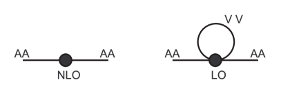
FIG. 11.: Diagrams contributing to $\Sigma_{N}$. The letters next to the lines denote the flavor indices of the propagating mesons. “LO” and “NLO” describe the order of the vertex that makes the diagram contribute at NLO.

The diagrams contributing to $\Sigma_{N}$ are of the general form shown in Fig. 11. The tree level contributions come from the two-meson vertices included in ${\mathcal{L}}_{NLO,2}$ [Eq. (9)]. The $v_{2}$ term acts as a subleading correction to $m_{0}^{2}$. Since at LO [Eq. (57)], ${\mathcal{D}}$ is independent of $m_{0}^{2}$, it follows that at NLO ${\mathcal{D}}$ can at most depend on its leading value. Thus $v_{2}$ contributes only at NNLO. The other tree level diagram comes from the $L_{7}$ term which gives the following contributions:

$$\delta^{(1)}x={8\over f^{2}}2L_{7}\chi_{A}^{2}\,,\quad\delta^{(1)}y={8\over f^{2}}2L_{7}\chi_{A}\chi_{S}\,,\quad\delta^{(1)}z={8\over f^{2}}2L_{7}\chi_{S}^{2}\,.$$ (B12)

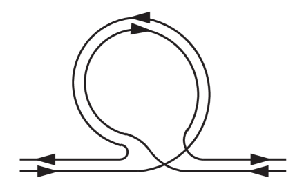
FIG. 12.: Each line in the diagram represents a single quark field. This is the only loop diagram of the type that appears in Fig. 11 in which the quark lines are disconnected.

Figure 12 shows the quark line structure of the only one-loop graph involving the lowest order vertices which corresponds to disconnected quark lines, and so does not contribute to $\Sigma_{C}$. The contribution to $\Sigma_{N}$ is

$$\delta^{(2)}x = {1\over 16\pi^{2}f^{2}}{1\over 3}(p^{2}-2\chi_{A})\chi_{A}\log\chi_{A}\,,$$ (B13)

$$\delta^{(2)}y = {1\over 16\pi^{2}f^{2}}{1\over 3}(p^{2}-\chi_{A}-\chi_{S}){\chi_{A}+\chi_{S}\over 2}\log\left({\chi_{A}+\chi_{S}\over 2}\right)\,,$$ (B14)

$$\delta^{(2)}z = {1\over 16\pi^{2}f^{2}}{1\over 3}(p^{2}-2\chi_{S})\chi_{S}\log\chi_{S}\,.$$ (B15)

Collecting these contributions we end up with

$$G^{-1}=\left(\begin{array}[]{ccc}v+x&\sqrt{N}y&-x\\ \sqrt{N}y&w+Nz&-\sqrt{N}y\\ -x&-\sqrt{N}y&-v+x\end{array}\right)\,.$$ (B19)

The relevant part of the inverse is

$$G_{AA}={1\over v}-{1\over v^{2}}{xw+N(xz-y^{2})\over w+Nz}\,.$$ (B20)

The first term is the one-loop corrected single pole, while the second contains the expected double pole. Inserting this result into the definitions Eqs. (52) and (55), and using Eqs. (B1) and (B5), we can read off the required double-pole coefficient

$${\cal D} = -{\cal Z_{A}}\left({xw+N(xz-y^{2})\over w+Nz}\right)\bigg{|}_{p^{2}=-M_{AA}^{2}}\,.$$ (B21)

Expanding in powers of $\chi$ we find

$${\cal D} \approx -{\cal Z_{A}}\left\{{w\over N}\left(1-{w\over Nx_{0}}\right)+(\delta x+\delta z-2\delta y)\right\}\bigg{|}_{p^{2}=-M_{AA}^{2}}\,.$$ (B22)

Note that $(x_{V}z_{V}-y_{V}^{2})=0$, so that a possible contribution proportional to $m_{0}^{2}$ cancels. Substituting and rearranging, we find the answer Eq. (59).

REFERENCES

- [1] A.G. Cohen, D.B. Kaplan and A.E. Nelson, JHEP 9911, 027 (1999).
- [2] S. Sharpe and N. Shoresh, Nucl. Phys. B (Proc. Suppl.) 83-84, 968 (2000).
- [3] C.W. Bernard and M.F.L. Golterman, Phys. Rev. D49, 486 (1994).
- [4] S. Sharpe, Phys. Rev. D56, 7052 (1997).
- [5] M.F.L. Golterman and K.C. Leung, Phys. Rev. D57, 5703 (1998); Nucl. Phys. B (Proc. Suppl.) 73, 246 (1999).
- [6] C. Chow and S. Rey, Nucl. Phys. B528, 303 (1998).
- [7] C. Chow and S. Rey, hep-ph/9712528.
- [8] S. Sharpe and Y. Zhang, Phys. Rev. D53, 5125 (1996).
- [9] S. Sharpe and N. Shoresh, in preparation.
- [10] A. Morel, J. Physique 48, 1111 (1987).
- [11] C.W. Bernard and M.F.L. Golterman, Phys. Rev. D46, 853 (1992).
- [12] J.F. Donoghue, E. Golowich and B.R. Holstein, “Dynamics of the standard model,” Cambridge Univ. Pr. (1992).
- [13] S. Sharpe and R.J. Singleton, Jr. Phys. Rev. D58, 074501 (1998).
- [14] M. Lüscher, S. Sint, R. Sommer and P. Weisz, Nucl. Phys. B478, 365 (1996).
- [15] S. Sharpe, Proc. 29th Int. Conf. on High Energy Physics, Vancouver, Canada, July 1998, p.171, eds. A. Astbury, D. Axen and J. Robinson (hep-lat/9811006).