Deconfinement transition and string tensions in SU(4) Yang-Mills Theory

Abstract

We present results from numerical lattice calculations of SU(4) Yang-Mills theory. This work has two goals: to determine the order of the finite temperature deconfinement transition on an $N_{t}=6$ lattice and to study the string tensions between static charges in the irreducible representations of SU(4). Motivated by Pisarski and Tytgat’s argument that a second-order SU($\infty$) deconfinement transition would explain some features of the SU(3) and QCD transitions, we confirm older results on a coarser, $N_{t}=4$, lattice. We see a clear two-phase coexistence signal in the order parameter, characteristic of a first-order transition, at $8/g^{2}=10.79$ on a $6\times 20^{3}$ lattice, on which we also compute a latent heat of $\Delta\epsilon\approx 0.6\epsilon_{\rm SB}$. Computing Polyakov loop correlation functions we calculate the string tension at finite temperature in the confined phase between fundamental charges, $\sigma_{1}$, between diquark charges, $\sigma_{2}$, and between adjoint charges $\sigma_{4}$. We find that $1<\sigma_{2}/\sigma_{1}<2$, and our result for the adjoint string tension $\sigma_{4}$ is consistent with string breaking.

I Introduction

It is well-established that the dynamics of the strong force are described by nonabelian gauge theory with an internal SU(3) symmetry and matter in the fundamental representation. Although the full theory of QCD contains dynamical quarks, study of SU(3) pure Yang-Mills theory ref:YANG_MILLS provides useful physical information. For example, in the valence or quenched approximation where gauge field configurations are generated without including the fermion determinant in the partition function, the computed light hadron spectrum differs from the experimentally measured spectrum at the 10% level ref:CPPACS_LAT98 . This is convenient since Monte Carlo calculations require enormous computational effort to include dynamical quark effects, so many studies are done in the quenched approximation in the interest of practicality. In the present paper we are interested in the phase diagram of QCD in the temperature–quark mass plane, and so the study of pure Yang-Mills theory covers the $m_{q}=\infty$ line.

The confinement–deconfinement transition of QCD at high temperature ($T\approx 100{\rm-}300$ MeV) has been studied with and without dynamical quarks and depends strongly on the number of light quark flavors and their masses. Pure gauge theory is recovered in the limit of infinite quark masses. In this limit the order parameter of the deconfinement transition is the Polyakov loop ref:POLY_SUSS ,

$$L(\vec{x})={1\over N_{c}}~{}{\rm Tr}~{}\prod_{t=1}^{N_{t}}U_{0}(\vec{x},t).$$ (1)

In the confined phase $\langle L\rangle_{\vec{x}}=0$, but in the deconfined phase the Polyakov loop acquires a nonzero expectation value, spontaneously breaking the global Z($N_{c}$) center symmetry. Since a Z(3) symmetry admits a cubic term in the effective potential, it drives a first-order transition; such is not the case for $N_{c}>3$ ref:SVET_YAFFE .

For $N_{f}$ flavors of massless quarks, the QCD Lagrangian has a global SU$(N_{f})_{L}\otimes$SU$(N_{f})_{R}$ chiral symmetry. At zero temperature this symmetry is spontaneously broken and the pions are the massless Goldstone bosons, but at some finite temperature $T_{\chi}$ the chiral symmetry is restored. Universality arguments suggest that the transition should be first-order for $N_{f}\geq 3$ ref:PIS_WIL , while a second-order transition for $N_{f}=2$ is not ruled out ref:WIL_RAJ (in fact a second-order transition is supported by lattice studies ref:KARSCH_LAT99 ). In nature the strange quark mass, $m_{s}$, is roughly 25 times larger than the average of up and down quark masses, $m_{u,d}=(m_{u}+m_{d})/2$. According to lattice calculations, the order of this “2+1” flavor phase transition depends on the strange mass. As $m_{s}$ is increased from $m_{u,d}$, the first-order phase transition weakens into a crossover ref:CU_2P1 . In Fig. 1 we reproduce the “Columbia” phase diagram which shows the order of the transition for different regions in $(m_{u,d},m_{s})$ plane.

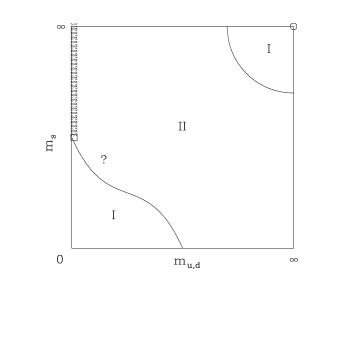
Figure 1: Columbia diagram ref:CU_2P1 , showing the nature of the 2+1-flavor finite temperature transition for different values of $m_{u,d}$ and $m_{s}$. Regions labeled I have a first-order transition, while the region II has only a crossover. For $m_{u}=m_{d}=0$ there is a tri-critical point (square) above which the chiral transition is second-order, denoted by asterisks. The pure glue limit is indicated by the octagon at $(\infty,\infty)$. The question mark indicates the physical $(m_{u,d},m_{s})$ according to calculations with staggered fermions ref:KS_2P1 . (Ref. ref:WIL_2P1 suggests that the physical point lies lower, in the Region I, when Wilson fermions are used.)

Recently Pisarski and Tytgat ref:PISARSKI_TYTGAT argued that the Columbia diagram is hard to understand in light of intuitive large-$N_{c}$ arguments. They point out that since anomaly effects are suppressed by $1/N_{c}$, the contribution of chiral symmetry restoration to the free energy is $O(N_{c})$ while the change in the free energy due to deconfinement is $O(N_{c}^{2})$. So, in the large-$N_{c}$ limit a first-order deconfinement transition should be robust for any quark mass. Thus, if the the first-order transition of SU(3) is a general feature of SU($N_{c}$) it is hard to understand why it disappears as the quark masses increase away from zero. One resolution of this conflict, they propose, is that $N_{c}=3$ is special due to the cubic term in the effective potential, and that the general SU($N_{c}$) deconfinement transition is second order.

Yang-Mills theory with $N_{c}$ colors, SU($N_{c}$) pure-gauge theory, has been a topic of exploration for lattice Monte Carlo study since the first days of the field ref:CREUTZ_SU2 . A first-order phase transition in the average energy was observed on symmetric lattices with volumes between $3^{4}$ and $6^{4}$ for $N_{c}=2-5$ ref:BALIAN ; ref:CREUTZ_SU2 ; ref:CREUTZ_SU3 ; ref:BCM ; ref:CREUTZ_SU5 . Refs. ref:BHANOT_CREUTZ ; ref:BKL ; ref:DHN demonstrated this transition is the consequence of a lattice-induced critical line separating the strong and weak coupling regimes. Specifically, they added to the usual fundamental single-plaquette action

$$S_{f}~{}=~{}-\frac{\beta}{6}\sum_{x}\sum_{\mu,\nu:\mu<\nu}{\rm Re~{}Tr}_{f}~{}P_{\mu\nu}(x)$$ (2)

the adjoint action

$$S_{A}~{}=~{}-\frac{\beta_{A}}{6}\sum_{x}\sum_{\mu,\nu:\mu<\nu}{\rm Re~{}Tr}_{A}~{}P_{\mu\nu}(x),$$ (3)

where $P_{\mu\nu}(x)$ is the plaquette $U^{\dagger}_{\nu}(x)U^{\dagger}_{\mu}(x+\hat{\nu})U_{\nu}(x+\hat{\mu})U_{\mu}(x)$ and Tr_f and Tr_A are traces in the fundamental and adjoint representations, respectively; $\mu$ and $\nu$ are space–time (or space–temperature) indices. Figure 2 shows the resulting phase diagram for this mixed action for SU(3) and SU(4). A first-order transition line separates the strong and weak coupling regimes of the fundamental coupling $\beta$. For $N_{c}\leq 3$ this line ends in a critical point before crossing the $\beta_{A}=0$ axis, but does cross this axis for $N_{c}>3$. Also displayed is the $\beta\approx 0$ transition line corresponding to the transition in SO($N_{c}^{2}-1$) gauge theory.

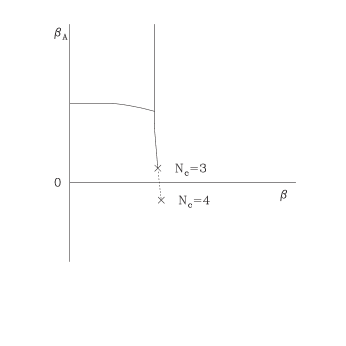
Figure 2: Phase diagram of fundamental-adjoint lattice action showing the lattice-induced bulk transition. The transition line crosses the fundamental axis for $N_{c}>3$.

This lattice-induced ($4d$) bulk transition, while interesting, can obscure the physical ($3d$) finite temperature transition of interest here. If the two transitions are nearby in parameter space, the first-order nature of the bulk transition would have a non-trivial effect on the confinement-deconfinement transition. The bulk transition was found to occur near $\beta=10.2$ (with $\beta_{A}=0$) ref:BHANOT_CREUTZ . The past finite temperature studies of SU(4) ref:GOCKSCH_OKAWA ; ref:GREEN_KARSCH ; ref:BAT_SVET ; ref:WHEAT_GROSS addressed this issue to varying degrees. For example, Ref. ref:BAT_SVET studied the deconfinement transition along the line $\beta_{A}=-\beta/2$, hoping to avoid crossing the bulk transition line. Ref. ref:WHEAT_GROSS found evidence on small volumes and $\approx 1000$ Monte Carlo evolution sweeps for deconfinement transitions for both $N_{t}=4$ and $N_{t}=5$ around $\beta=10.5$ and $\beta=10.6$ (with $\beta_{A}=0$). All these studies concluded that the SU(4) deconfinement transition was first-order. However, given the alluring explanation for the Columbia diagram, we felt the time was ripe to revisit finite temperature SU(4) numerically.

Another topic which we address in this work is the tension of confining strings which carry $k\in\{1,...,N_{c}\}$ units of flux. Only for $N_{c}>3$ can one find different strings with unequal tensions. With these finite-temperature calculations we find the ratio of diquark ($\sigma_{k=2}$) to fundamental ($\sigma_{k=1}$) string tensions to be in the range $1<\sigma_{k=2}/\sigma_{k=1}<2$. As pointed out in Ref. ref:STRASSLER , these types of computations may test dualities between gauge theories and string theories. String tensions can be computed on the lattice, in broken supersymmetric gauge theory, and in M theory versions of QCD and supersymmetric QCD. Our result for $\sigma_{2}/\sigma_{1}$ indicates that in SU(4) Yang-Mills flux tubes attract each other as expected from SUSY Yang-Mills and M theory ref:STRASSLER and proved in standard Yang-Mills ref:CREUTZ_PRIVATE .

In the next Section we describe some details of our calculations. Section III gives the results for the deconfinement transition, and Section IV shows our calculation of the string tensions. Finally we summarize our results in Section V.

II Computation

Our calculations of SU(4) Yang-Mills theory do not differ significantly from standard SU(3) calculations. We use the fundamental single-plaquette action, Equation (2), with $\beta=2N_{c}/g^{2}=8/g^{2}$. Our production code is a minimally modified version of the MILC code ref:MILC_CODE . Our algorithm for evolving the gauge fields is a mixed overrelaxation/heatbath procedure: in one Monte Carlo “sweep” we perform 10 microcanonical overrelaxation steps followed by one Kennedy-Pendleton ref:KEN_PEND heatbath step. Each sweep we compute the average plaquette and fundamental Polyakov loop. We generate at least 1000 Monte Carlo sweeps at each $\beta$, with 10000 to 20000 sweeps around $\beta_{c}$. An independent Metropolis code was written from scratch for SU(4) to check this MILC-derived SU(4) code.

For those values of the coupling $\beta$ where we want to calculate the string tension, we compute correlation functions of Polyakov loops in the irreducible representations of SU(4)

$$C_{i}(r)=\langle L_{i}(\vec{x})L_{i}^{*}(\vec{x}+\vec{r})\rangle_{\vec{x}},$$ (4)

where $i$ =4, 6, 10 and 15 and the trace in Eq. (1) is $i$-dimensional. As is well known, the diquark 6 and 10 representations are obtained by antisymmetrizing and symmetrizing two fundamental 4 representations, and the adjoint 15 by inserting SU(4) Gell-Mann matrices. We use the Parisi-Petronzio-Rapuano multihit variance reduction method ref:PPR to reduce noise. Polyakov loop correlation functions are computed every tenth Monte Carlo sweep. We investigate autocorrelations by including only every $n$-th configuration, where $n=1$, 5, and 10. We have a total of 2800 measurements for the calculations on a $6\times 16^{3}$ lattice and 1900 measurements for the calculations on a $8\times 12^{3}$ lattice.

III Deconfinement transition

In order to make contact with previous finite temperature SU(4) calculations, we compute thermodynamic observables on a $4\times 8^{3}$ lattice for values of $\beta=8/g^{2}$ between 10.0 and 10.6. We find a rapid change in $\langle|L|\rangle$ between $\beta=10.45$ and $\beta=10.5$ (see Fig. 3), in agreement with Refs. ref:GOCKSCH_OKAWA ; ref:WHEAT_GROSS . Since the plaquette is also increasing in that region (Fig. 4), one might worry that the bulk transition is affecting the deconfinement transition. Therefore, we did not pursue confirming the order of the deconfinement transition with $N_{t}=4$, and instead focus on $N_{t}=6$ where the bulk and deconfinement transitions should be further separated.

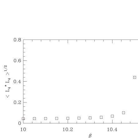
Figure 3: Magnitude of the Polyakov loop vs. $\beta$ on a $4\times 8^{3}$ lattice.

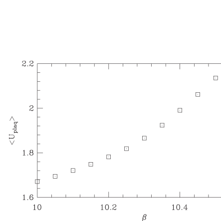
Figure 4: Plaquette vs. $\beta$ on $4\times 8^{3}$ lattice. The normalization is such that $\langle U_{\mathrm{plaq}}\rangle=N_{c}$ in the free theory.

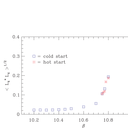
Figure 5: Magnitude of the fundamental Polyakov loop vs. $\beta$ on a $6\times 12^{3}$ lattice.

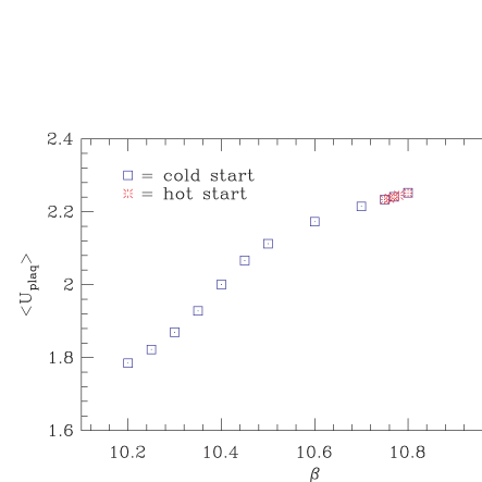
Figure 6: Plaquette vs. $\beta$ on a $6\times 12^{3}$ lattice. The normalization is such that $\langle U_{\mathrm{plaq}}\rangle=N_{c}$ in the free theory.

In our $6\times 12^{3}$ calculations we find that the jump in $\langle|L|\rangle$ is between $\beta=10.75$ and $\beta=10.80$ (Fig. 5). This move in $\beta$ of the critical point is consistent with the conjecture that the deconfinement is a thermodynamic phenomenon. On the other hand the increase in the plaquette is over the same $\beta$ (10.2-10.6) region as for $N_{t}=4$ (see Fig. 6), as is expected for a bulk transition. And with $N_{t}=6$ the bulk and finite-temperature phase transitions are clearly separated.

The six plots shown in Fig. 7 show the real and imaginary parts of the Polyakov loop for the last 2000 sweeps of calculations at the corresponding couplings. One can see the spontaneous breaking of the Z(4) symmetry as the deconfinement transition is crossed.

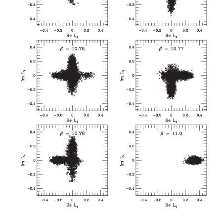
Figure 7: Plots at six values of $\beta$ showing the phase and magnitude of the average fundamental Polyakov loop on consecutive $6\times 12^{3}$ configurations. Each cross corresponds to the value of $L_{4}$ computed on a single configuration.

One quantitative estimation of the critical coupling, $\beta_{c}$, comes from the deconfinement fraction ref:CT . Let us define $\phi\in[0,\pi/4]$ as the angle between arg($L_{4}$) and the nearest Z(4) symmetry axis. Given another angle $\theta\in[0,\pi/4]$, one counts the number of configurations where $\phi\leq\theta$, $N_{in}$, versus the number of configurations where $\phi>\theta$, $N_{out}$. In the confined, Z(4)-symmetric phase, on average,

$${N_{in}\over N_{in}+N_{out}}~{}=~{}{\theta\over(\pi/4)}.$$ (5)

The deconfinement fraction is the excess number of configurations which have $\phi\leq\theta$:

$$f(\theta)~{}\equiv~{}{\pi/4\over(\pi/4)-\theta}\bigg{[}{N_{in}\over N_{in}+N_{out}}~{}-~{}{\theta\over(\pi/4)}\bigg{]},$$ (6)

where the factor outside the brackets normalizes the totally deconfined $f(\theta)$ to one. (Note that due to statistical fluctuations, $f(\theta)$ can be slightly negative in the confined phase.) The critical coupling is defined to be the value of $\beta$ for which $f(\theta)=1/2$.

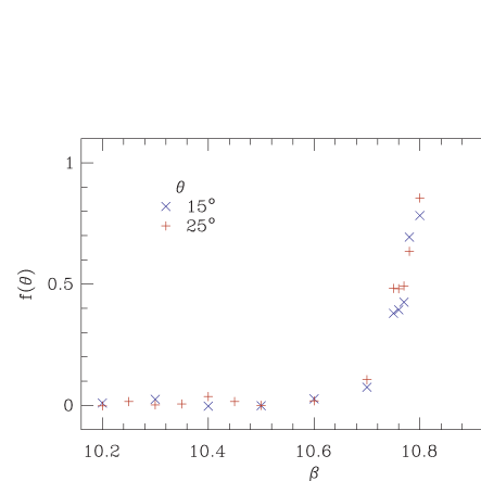
Figure 8: Deconfinement fraction (defined in text) vs. $\beta$ for the $6\times 12^{3}$ lattice.

In Fig. 8 we plot the deconfinement fraction with $\theta=15^{\circ}$ and $25^{\circ}$ for the $6\times 12^{3}$ lattice. We find $\beta_{c}=10.78\pm 0.01$, where the uncertainty is estimated by varying $\theta$ between $15^{\circ}$ and $30^{\circ}$.

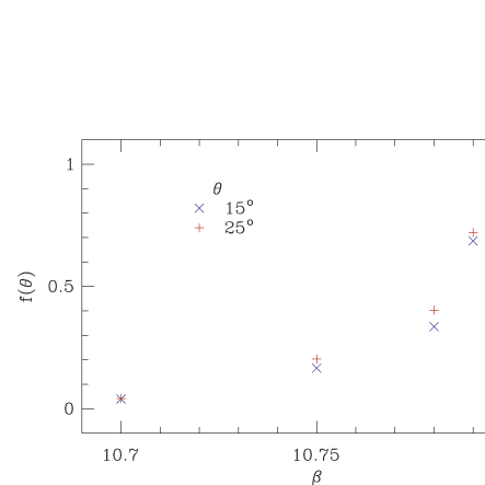
Figure 9: Deconfinement fraction vs. $\beta$ for the $6\times 16^{3}$ lattice.

In order to determine the order of the phase transition, we increased the spatial volume to $16^{3}$ and $20^{3}$. With the larger volumes, the critical coupling increases slightly to $\beta_{c}=10.79$ as is expected (see Fig.9). The histograms of Polyakov loop magnitude $|\langle L_{4}\rangle|$ obtained from the larger two lattice volumes near their respective critical points show two peaks, in clear contrast to the $12^{3}$ volume. See Figure 10. This suggests a first-order phase transition.

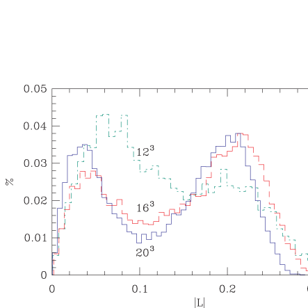
Figure 10: Histogram of $|L_{4}|$ at $\beta_{c}=10.78,10.79,10.79$ on volumes of $12^{3},16^{3},20^{3}$, respectively.

Indeed Polyakov loop evolution in simulation time, in Figure 11, signals coexistence of the confined and deconfined phases at this temperature, $\beta=10.79$. The magnitude stays with its low (confined) or high (deconfined) value for a relatively long period, but occasionally jumps very quickly from one to the other value. And when the magnitude is low, the argument takes random arbitrary values, while it is fixed to the neighborhood of one of the four allowed Z(4) values when the magnitude is high.

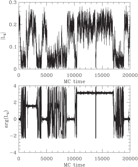
Figure 11: Monte Carlo evolution of the magnitude (top) and the argument (bottom) of the fundamental Polyakov loop for $\beta=10.79$ on the $6\times 20^{3}$ volume. We take ${\rm arg}(L_{4})\in[-\frac{3\pi}{4},\frac{5\pi}{4}]$ for clarity.

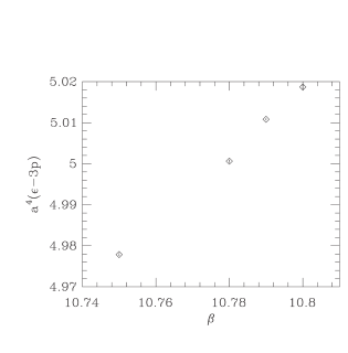
Figure 12: Energy density minus 3 times the pressure vs. $\beta$ for the $6\times 16^{3}$ lattice. A divergent vacuum contribution remains to be subtracted.

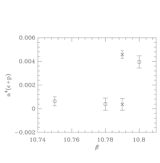
Figure 13: Energy density plus pressure vs. $\beta$ for the $6\times 16^{3}$ lattice. Squares correspond to averaging over the whole data set, the fancy crosses at the critical beta correspond to separating into hot and cold phases as described in the text.

By combining these histogram and evolution observations, we conclude that the finite-temperature deconfining phase transition of SU(4) Yang-Mills system is of first-order. It is thus desirable to compute the latent heat through combinations of the energy density $\epsilon$ and the pressure $p$ Engels:1982qx . Specifically we compute

$$a^{4}(\epsilon-3p) = -{6N_{c}}a\frac{\partial g^{-2}}{\partial a}(\overline{P_{t}}+\overline{P_{s}})$$ (7)

$$a^{4}(\epsilon+p) = \frac{8N_{C}}{g^{2}}C(g^{2})(\overline{P_{t}}-\overline{P_{s}})\,.$$ (8)

The average space-space and space-time (or space-temperature) plaquettes are normalized such that if $g^{2}=0$, $\overline{P_{t}}=\overline{P_{s}}=1$:

$$\overline{P_{t}} = \frac{1}{3\Omega}\frac{1}{N_{c}}\sum_{x}\sum_{i}{\rm Re~{}Tr}_{f}P_{0i}(x)$$ (9)

$$\overline{P_{s}} = \frac{1}{3\Omega}\frac{1}{N_{c}}\sum_{x}\sum_{i,j:i<j}{\rm Re~{}Tr}_{f}P_{ij}(x)$$ (10)

where $\Omega$ is the $4d$ volume and $i$ and $j$ are spatial indices. In bare lattice perturbation theory the $\beta-$function and Karsch coefficient are given, respectively, by Karsch:1982ve

$$a\frac{\partial g^{-2}}{\partial a}=-2\frac{11N_{c}}{3(16\pi^{2})}+O(g^{2})$$ (11)

and

$$C(g^{2})=1 - \left[4N_{c}\left(\frac{N_{c}^{2}-1}{32N_{c}^{2}}0.586844-0.005306\right)\right.$$ (12)

$$+ \left.\frac{11N_{c}}{6(16\pi^{2})}\right]g^{2}$$

It is possible, and advisable, to use mean-field improved perturbation theory or a nonperturbative calculation of these quantities for an accurate calculation of the energy and pressure Boyd:1996bx ; however, for the purpose of establishing a nonzero latent heat, bare perturbation theory suffices.

The quantities $\epsilon-3p$ and $\epsilon+p$ are plotted as functions of $\beta$ on the $16^{3}$ lattice and shown in Figures 12 and 13, respectively. The fancy crosses in the latter figure correspond to separating the configurations at $\beta_{c}=10.79$ into hot and cold phases. Note that $\epsilon-3p$ plotted in Fig. 12 contains a divergent vacuum contribution which may be subtracted after a zero temperature simulation is performed; however, such subtraction is not necessary in order to compute the latent heat from a discontinuity in $\epsilon-3p$ at the critical coupling $\beta_{c}$. The separation of phases at $\beta_{c}$ was made on the basis of whether $|L_{4}|$ was greater or lesser than some value $r$. Based on the histograms in Fig. 10 we varied $r$ from 0.08 to 0.14. Table 1 lists the values for $\Delta(\epsilon-3p)$ and $\Delta(\epsilon+p)$ obtained for different $r$ on both the $16^{3}$ and $20^{3}$ volumes. The variation as a function of $r$ is within the statistical errors.

Thus, we observe a latent heat which is many standard deviations greater than zero. We also see that $\Delta(\epsilon-3p)\neq\Delta(\epsilon+p)$ which implies a discontinuous change in pressure across the transition. If, for example, we take the $6\times 20^{3}$ data with $r=0.10$, we find (with statistical errors only)

$$\Delta\epsilon = 5.7(3)T_{c}^{4}$$ (13)

$$\Delta p = -0.45(13)T_{c}^{4}\,.$$ (14)

A nonzero $\Delta p$ was also seen in early studies of SU(3) Svetitsky:1983bq ; Brown:1988qe and disappeared when going from the perturbative estimates for (11) and (12) to nonperturbative calculations Boyd:1996bx .

Table 1: Discontinuities in $\epsilon-3p$ and $\epsilon+p$ at $\beta=10.79$ for various values of $r$ (described in text). The lattice spacing has been set through the critical temperature: $a(\beta_{c})=(N_{t}T_{c})^{-1}$.

$\Omega$	$r$	$\Delta(\epsilon-3p)/T_{c}^{4}$	$\Delta(\epsilon+p)/T_{c}^{4}$
$6\times 16^{3}$	0.08	$7.5(4)$	$4.8(8)$
	0.10	$7.6(4)$	$5.4(8)$
	0.12	$7.6(4)$	$5.3(8)$
	0.14	$7.6(4)$	$5.7(8)$
$6\times 20^{3}$	0.08	$6.7(3)$	$4.9(4)$
	0.10	$7.0(3)$	$5.2(4)$
	0.12	$7.0(3)$	$5.3(4)$
	0.14	$7.1(3)$	$5.4(4)$

A thorough calculation of the latent heat in the SU(4) deconfinement transition requires a full study of the lattice spacing dependence as well as nonperturbative determination of the $\beta$-function and Karsch coefficient. However, even the exploratory study here makes clear the latent heat is nonzero and further establishes the first-order nature of the phase transition.

We can compare the latent heat for SU(4) to that for SU(3) by normalizing by the energy density for an ideal gluon gas. If we take the latent heat to be $\Delta\epsilon/T_{c}=6.0\pm 1.5$ and divide by the Stefan–Boltzmann energy density,

$$\epsilon_{\rm SB}(T)~{}=~{}\frac{(N_{c}^{2}-1)\pi^{2}}{15}T^{4}$$ (15)

we find

$$\frac{\Delta\epsilon}{\epsilon_{\rm SB}(T_{c})}~{}=~{}0.60\pm 0.15\,.$$ (16)

Our result should be compared against the $N_{t}=6$ SU(3) latent heat obtained using a perturbative $\beta-$function: $\Delta\epsilon/\epsilon_{\rm SB}=0.454(11)$ Beinlich:1997xg . A state-of-the-art SU(3) calculation, which used an improved action and a nonperturbative $\beta-$function, gave $\Delta\epsilon/\epsilon_{\rm SB}=0.266(17)$ Beinlich:1997xg . Further work is required to see if the effect of going from a perturbative to nonperturbative $\beta-$function is as dramatic for SU(4) as for SU(3).

IV String tensions

Figure 14: Polyakov loop correlation function in 4 (top) and 6 (bottom) representations on a $6\times 16^{3}$ lattice at $\beta=10.65$. The symbols are the data points and the solid lines are fits in the range $4\leq r\leq 12$.

Figure 15: Polyakov loop correlation function in 4 (top) and 6 (bottom) representations on a $6\times 16^{3}$ lattice at $\beta=10.70$. The symbols are the data points and the solid lines are fits in the range $5\leq r\leq 11$.

Table 2: String tensions (in lattice units) between static fundamental ($k=1$) and diquark ($k=2$) charges, and their ratio, using every $(N_{\rm skip}+1)$th configuration in the analysis. The quoted uncertainties are statistical.

$\beta$	$N_{\rm skip}$	$\sigma_{1}$	$\sigma_{2}$	$\sigma_{2}/\sigma_{1}$
	0	0.098(2)	0.138(14)	1.45(15)
10.65	4	0.092(4)	0.137(30)	1.67(36)
	9	0.101(7)	0.164(56)	1.77(67)
	0	0.076(2)	0.118(13)	1.59(13)
10.70	4	0.080(4)	0.154(40)	1.91(49)
	9	0.084(6)	0.163(53)	2.03(68)

We use two different lattices, $6\times 16^{3}$ and $8\times 12^{3}$, for studying string tensions. For the former, we choose the coupling values of $\beta$=10.65 and 10.70, safely away from both the bulk and the deconfining phase transitions, and in the confining phase (see Figure 7). Polyakov loop correlations (see Eq. (4)) for the fundamental (4, $k=1$, top) and anti-symmetric diquark (6, $k=2$, bottom) representations are shown in Figures 14 and 15. A clear difference in the rates of exponential decay is observed between $C_{\bf 4}$ and $C_{\bf 6}$. Using a correlated, jackknifed fit to the form ref:FSST

$$\frac{a_{k}}{r}\exp[-V_{k}(r)N_{t}]+\frac{a_{k}}{N_{s}-r}\exp[-V_{k}(N_{s}-r)N_{t}],$$ (17)

with $N_{t}=6$, $N_{s}=16$ and

$$V_{k}(r)=\sigma_{k}r-\frac{\pi r}{3N_{t}^{2}}$$ (18)

we obtain string tensions, $\sigma_{1}$ and $\sigma_{2}$, and their ratio, tabulated in Table 2. The analysis of the correlation functions is done using every measurement, every fifth measurement, and every tenth measurement in order to estimate correlations between successive measurements (each separated by 10 Monte Carlo steps, see Sec. II). The increase in the statistical error with the number of skipped configurations, $N_{\rm skip}$, indicates a significant auto-correlation. Unfortunately, it appears that several hundred configurations are necessary in order to obtain a precise fit, so we cannot drop too many of the measurements. However, we can infer from our data that

$$\frac{\sigma_{2}}{\sigma_{1}}>1\,,$$ (19)

by roughly 2 standard deviations. Note that both $\sigma_{1}$ and $\sigma_{2}$ decrease as $\beta\to\beta_{c}$ (i.e. as $T$ increases). Since the lattice spacing decreases as $T$ increases, the fit range for $\beta=10.70$ does not include the $r=4$ and $r=12$ data (see captions of Figs. 14 and 15). Our numerical accuracy is good enough to conclude there are two different strings, one between the fundamental charges carrying one unit of flux, and another, stronger, between the diquark charges carrying two units of flux. It is not yet good enough, however, to distinguish among various predictions for this ratio summarized by Strassler ref:STRASSLER . However, this establishes numerically the expectation for $\sigma_{1}\neq\sigma_{2}$ in SU(4) Yang-Mills theory, just as Ref. Ohta:1986pc showed $\sigma_{1}=\sigma_{2}$ in SU(3) Yang-Mills theory.

A string model ref:PISARSKI_ALVAREZ predicts that

$$\frac{T_{c}}{\sqrt{\sigma_{1}(T=0)}}\approx\sqrt{\frac{3}{\pi(d-2)}}=0.69\,,$$ (20)

which is quite close for SU(3) ref:KARSCH_LAT99 . We have not computed the zero temperature string tension, but only the string tension roughly near $T_{c}$, to find

$$\frac{T_{c}}{\sqrt{\sigma_{1}(T\approx T_{c})}}=0.60\,.$$ (21)

The extent which the lattice scale changes between $\beta=10.70$ and $\beta_{c}=10.79$ is main uncertainty above. Of course a zero temperature study is necessary before one can assess the agreement with Eq. (20).

On this lattice of $6\times 16^{3}$, which is coarser and larger of the two, no signal was obtained for either the symmetric diquark (10) or adjoint (15) representations. In contrast, with the finer lattice spacing (at $\beta=10.85$) on the smaller $8\times 12^{3}$ lattice, flattening of the adjoint correlation is observed (see Figure 16). This suggests the breaking of confining string for the adjoint representation at a rather short distance of 3 lattice spacings. It gives us confidence that the correlations on the $6\times 16^{3}$ lattice should be dominated by the non-perturbative strings for ranges longer than at least 3 lattice units. Notice also that while string breaking is an expected behavior for the adjoint representations in general ref:STRINGBREAKING , such an absence of string is yet to be observed in SU(3) Yang-Mills theory which employs much finer and larger lattices than the present work.

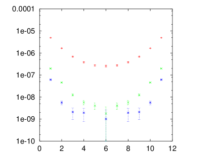
Figure 16: Polyakov loop correlation function in 4 (top), 6 (middle), and 15 (bottom) representations on a $12^{3}\times 8$ lattice at $\beta=10.85$

V Conclusions

We have revisited the confinement–deconfinement transition of SU(4) Yang-Mills theory through Monte Carlo lattice calculation. One problem with the earlier results is that the deconfinement transition with $N_{t}=4$ is very close in coupling constant space to a known bulk transition, so that its finite-temperature nature or its order is not clear. We have shown that by decreasing the lattice spacing by $2/3$, the deconfinement transition moves upward in the coupling and proves itself as a finite-temperature transition, and it becomes well-separated from the bulk transition which does not move. Nevertheless, we observe a clear signal for coexistence of confined and deconfined phases at this deconfinement transition. Therefore, we confirm that the deconfinement transition of SU(4) Yang-Mills theory is first-order. Additionally a first calculation of the latent heat of the SU(4) deconfinement transition has been presented here, giving $\Delta\epsilon\approx 6T_{c}$, or $\Delta\epsilon/\epsilon_{\rm SB}\approx 0.6$. Using improved techniques, the SU(3) latent heat is $\Delta\epsilon/\epsilon_{\rm SB}=0.266(17)$ Beinlich:1997xg , and it will be interesting to see how the latent heat depends on $N_{c}$.

Our calculations of the string tensions are a first study in lattice SU(4) and should be improved to meet the current state-of-the-art which exists for SU(3). Even so, we observe a ratio for 4 and 6 dimensional string tensions which is between 1 and 2. It also appears that the adjoint string breaks at a short distance. We hope this work shows that it is interesting and feasible to study ratios of string tensions for $N_{c}>3$ lattice simulations.

References

- (1) C.N. Yang and R. Mills, Phys. Rev. 96, 191 (1954).
- (2) For Wilson fermion quarks, see e.g. R. Burkhalter, (CP-PACS Collaboration), in Lattice ’98, Proceedings of the “XVIth International Symposium on Lattice Field Theory,” Boulder, Colorado, edited by T. DeGrand et al., Nucl. Phys. B (Proc. Suppl.) 73, 3 (1999). For staggered fermion quarks, e.g. S. Kim and S. Ohta, Phys. Rev. D61, 074506 (2000).
- (3) A.M. Polyakov, Phys. Lett. 72B, 477 (1978); L. Susskind, Phys. Rev. D20, 2610.
- (4) B. Svetitsky and L.G. Yaffe, Nucl. Phys. B210 [FS6], 423 (1982).
- (5) R.D. Pisarski and F. Wilczek, Phys. Rev. D29, 338 (1984).
- (6) F. Wilczek, Int. J. of Mod. Phys. A7, 3911 (1992); K. Rajagopal and F. Wilczek, Nucl. Phys. B399, 395 (1993).
- (7) For a summary of recent finite temperature lattice QCD studies see review by F. Karsch, to appear in Lattice ’99, Proceedings of the “XVIIth International Symposium on Lattice Field Theory,” Pisa, Italy, Nucl. Phys. (Proc. Suppl.) 83-84, 14 (2000).
- (8) F.R. Brown et al., Phys. Rev. Lett. 65, 2491 (1990).
- (9) S. Aoki et al., (JLQCD Collaboration), in Lattice ’98, Proceedings of the “XVIth International Symposium on Lattice Field Theory,” Boulder, Colorado, edited by T. DeGrand et al., Nucl. Phys. B (Proc. Suppl.) 73, 459 (1999), hep-lat/9809102.
- (10) Y. Iwasaki et al., Phys. Rev. D54, 7010 (1996).
- (11) R.D. Pisarski and M. Tytgat, “Why the SU() deconfining transition might be of second order,” Proc. XXV Hirshegg Workshop on “QCD Phase Transition,” Jan., ’97, hep-ph/9702340.
- (12) R. Balian, M. Drouffe and C.Itzykson, Phys. Rev. D11, 2104 (1975).
- (13) M. Creutz, Phys. Rev. D21, 2308 (1980).
- (14) M. Creutz, Phys. Rev. Lett. 45, 313 (1980); M. Creutz and K.J.M. Moriarty, Phys. Rev. D26, 2166 (1982).
- (15) D. Barkai, M. Creutz and K.J.M. Moriarty, Nucl. Phys. B225 [FS9], 156 (1983).
- (16) M. Creutz, Phys. Rev. Lett. 46, 1441 (1981).
- (17) G. Bhanot and M. Creutz, Phys. Rev. D24, 3212 (1981).
- (18) R. Brower, D. Kessler, and H. Levine, Phys. Rev. Lett. 47, 621 (1981); Nucl. Phys. B205 [FS5], 77 (1982).
- (19) R. Dashen, U. Heller, and H. Neuberger, Nucl. Phys. B215 [FS7], 360 (1983).
- (20) A. Gocksch and M. Okawa, Phys. Rev. Lett. 52, 1751 (1984).
- (21) F. Green and F. Karsch, Phys. Rev. D29, 2986 (1984).
- (22) G.G. Batrouni and B. Svetitsky, Phys. Rev. Lett. 52, 2205 (1984).
- (23) J.F. Wheater and M. Gross, Phys. Lett. 144B, 409 (1984).
- (24) M.J. Strassler, in YKIS ’97, Proceedings of the “Yukawa International Seminar on Non-Perturbative QCD: Structure of the QCD Vacuum,” Prog. Theor. Phys. Suppl., 131, 439 (1998), hep-lat/9803009; and in Lattice ’98 Proceedings of the “XVIth International Symposium on Lattice Field Theory,” Boulder, Colorado, edited by T. DeGrand et al., Nucl. Phys. B (Proc. Suppl.) 73, p. 120, hep-lat/9810059; and references cited therein.
- (25) M. Creutz, private communication.
- (26) Public MILC code available at http://physics.indiana.edu/sg/milc.html.
- (27) A.D. Kennedy and B.J. Pendleton, Phys. Lett. 156B, 393 (1985).
- (28) G. Parisi, R. Petronzio, and F. Rapuano, Phys. Lett. 128B, 418 (1983).
- (29) N.H. Christ and A.E. Terrano, Phys. Rev. Lett. 56, 111 (1986).
- (30) J. Engels, F. Karsch, H. Satz and I. Montvay, Nucl. Phys. B205, 545 (1982).
- (31) F. Karsch, Nucl. Phys. B205, 285 (1982).
- (32) G. Boyd, J. Engels, F. Karsch, E. Laermann, C. Legeland, M. Lutgemeier and B. Petersson, Nucl. Phys. B469, 419 (1996).
- (33) B. Svetitsky and F. Fucito, Phys. Lett. B131, 165 (1983).
- (34) F. R. Brown, N. H. Christ, Y. F. Deng, M. S. Gao and T. J. Woch, Phys. Rev. Lett. 61 (1988) 2058.
- (35) B. Beinlich, F. Karsch and A. Peikert, Phys. Lett. B390, 268 (1997).
- (36) Ph. de Forcrand, G. Schierholtz, H. Schneider, and M. Teper, Phys. Lett. 160B, 137 (1985).
- (37) S. Ohta, M. Fukugita and A. Ukawa, Phys. Lett. B173, 15 (1986).
- (38) R. Pisarski and O. Alvarez, Phys. Rev. D26, 3735 (1982).
- (39) See C. Bernard, Nucl. Phys. B219, 341 (1983) for the original strong coupling analysis. A somewhat different large- view was presented in J. Greensite and M.B. Halpern, Phys. Rev. D27, 2545 (1983). And for a recent review see K. Schilling, in Lattice ’99 ref:KARSCH_LAT99 , p.140.