Heavy Quarks on Anisotropic Lattices:
The Charmonium Spectrum

Abstract

We present results for the mass spectrum of $c{\bar{c}}$ mesons simulated on anisotropic lattices where the temporal spacing $a_{t}$ is only half of the spatial spacing $a_{s}$. The lattice QCD action is the Wilson gauge action plus the clover-improved Wilson fermion action. The two clover coefficients on an anisotropic lattice are estimated using mean links in Landau gauge. The bare velocity of light $\nu_{t}$ has been tuned to keep the anisotropic, heavy-quark Wilson action relativistic. Local meson operators and three box sources are used in obtaining clear statistics for the lowest lying and first excited charmonium states of ${}^{1}S_{0}$, ${}^{3}S_{1}$, ${}^{1}P_{1}$, ${}^{3}P_{0}$ and ${}^{3}P_{1}$. The continuum limit is discussed by extrapolating from quenched simulations at four lattice spacings in the range 0.1 - 0.3 fm. Results are compared with the observed values in nature and other lattice approaches. Finite volume effects and dispersion relations are checked.

I Introduction

Lattice Quantum Chromodynamics (QCD) opens a gateway to the study of non-perturbative phenomena in the strong interaction world. To explain (and in some cases predict) why the elementary particles are as heavy as they are is not only exciting, it is also unavoidable in the validation of QCD as the standard model of the strong interactions. Unfortunately the lattice simulations are by no means cheap, it is typical for a project to take months or years to finish on the present fastest supercomputers.

The study of heavy quarks demands even more computing resources than that of light quarks, while heavy quarks may be more interesting. As standard lattice actions break down when the lattice spacing $a>\frac{1}{m_{0}}$, where $m_{0}$ is the bare quark mass, the imposition of a fine enough lattice spacing makes the studies of heavy quarks completely out of reach given current computing power. To treat heavy quarks, special lattice actions must be designed. The two dominant approaches are non-relativistic lattice QCD (NRQCD) and the heavy relativistic or Fermilab approach, and there is the newer anisotropic relativistic approach used in our work.

The NRQCD approach [1, 2] attempts to describe an effective field theory at low energy. Essentially the action is expanded in powers of the lattice spacing $a$, as standard lattice actions are, and in powers of the heavy quark velocity $v^{2}$. Practically the NRQCD method works well for the spin-independent $b{\bar{b}}$ system made of bottom quarks. However, continuum extrapolation is impossible in NRQCD as the non-relativistic expansion requires $am_{0}>1$. Also, to study spin splittings, higher order terms have to be added to the action. For the $c{\bar{c}}$ (charmonium) system, present evidence [3, 4] suggests that the NRQCD approach breaks down. The spin splittings in the charmonium spectrum do not converge when higher relativistic corrections are added to the non-relativistic action, or when quantum corrections are switched from one prescription to another.

The heavy-relativistic or Fermilab approach [5] incorporates interactions from both the small- and large-mass limits. For heavy quarks, the lattice action can be interpreted in a non-relativistic light. Yet as $m_{0}a\rightarrow 0$, the action conforms exactly to the standard Wilson action for light quarks. This is accomplished without any constraint on the value of $am_{0}$, in contrast to $am_{0}>1$ in NRQCD and $am_{0}\ll 1$ in Wilson action. The Fermilab approach connects both ends smoothly. Concretely, its lattice action up to $O(a^{2})$ lattice errors is simply the standard clover-term improved Wilson action without imposing space-time exchange symmetry. The coefficients in front of the covariant derivatives and the clover term improvement now appear in two copies, a temporal one and a spatial one. The difficulty is that, to achieve the elimination of $O(a)$ lattice artifact for heavy quarks, these coefficients must all be all mass dependent.

The anisotropic relativistic approach [6, 7] goes one step further. As in the heavy relativistic approach, the space-time exchange symmetry is not imposed on the lattice action. The key difference is, here in the anisotropic relativistic approach, the lattice itself is discretized differently along the temporal and spatial directions with the temporal spacing $a_{t}$ chosen finer than the spatial spacing $a_{s}$. Since no further symmetry besides the space-time exchange symmetry is broken, the anisotropic action has the same terms as the heavy relativistic action does. Defining the true anisotropy $\xi=\frac{a_{s}}{a_{t}}$ as the ratio of the spatial to the temporal spacing, we may consider the heavy relativistic approach as the $\xi=1$ special case of the anisotropic relativistic approach. In both approaches, the relativity of the lattice action is restored by a required tuning of the bare parameters in the action.

There is one obvious benefit of moving to an anisotropic lattice: heavy meson propagators often die out very fast and thus leave too few time slices which are useful for mass fitting. With a finer temporal lattice spacing, this problem may be cured at relatively low cost. Another equally important benefit is that, with $a_{t}m_{0}\ll 1$ on an anisotropic lattice, the mass dependence of the improvement coefficients can be expected to be weaker, or absent all together as is the case for some coefficients classically. Since the numerically determined clover coefficients deviate considerably from their perturbative estimates, their possible weak mass dependence may allow us to avoid a difficult, non-perturbative numerical determinations.

To be self-contained, now we review the theoretical framework laid out in [6, 7].

II The anisotropic Wilson QCD action

The anisotropic QCD action is the sum of the gauge action $S_{G}^{\xi}$ and the fermion action $S_{F}^{\xi}$

$$S^{\xi}=S_{G}^{\xi}+S_{F}^{\xi}\,.$$ (1)

A The anisotropic gauge action $S_{G}^{\xi}$

On an anisotropic lattice the gauge action becomes

$$S_{G}^{\xi} = \frac{\beta}{N_{c}}\left[\frac{1}{\xi_{o}}\sum_{x,s>s\prime}{\rm Re}\,{\rm Tr}\,\left[1-P_{ss\prime}(x)\right]+\xi_{o}\sum_{x,s}{\rm Re}\,{\rm Tr}\,\left[1-P_{st}(x)\right]\right]$$ (2)

where $\xi_{o}$ is the bare anisotropy, which equals to the true anisotropy $\xi=\frac{a_{s}}{a_{t}}$ only at the classical level. Note that the anisotropic $\beta$ is the geometric mean of the $\beta$’s along the temporal and spatial directions, thus it corresponds to a coarser spatial spacing and a finer temporal spacing than given by its isotropic equivalent of same value. Here $a_{s}$ and $a_{t}$ refer to the actual “physical” lattice spacings as computed by examining the propagation of physical particles over distances of many lattice units. Standard renormalization argument guarantee us that the resulting long distance physics predicted by the action in eq.(2) will appear consistent with relativity after this anisotropic interpretation of lattice scales is adopted.

It is suggested that the true anisotropy $\xi$ be fixed during the continuum extrapolation, for reasons shown later. All the computations are done at $\xi=2$ in this work. The bare anisotropy $\xi_{0}$ is tuned at each $\beta$ to keep $\xi$ the same [8].

B A few standard definitions

The covariant first- and second-order lattice derivatives $\nabla_{\mu}$ and $\Delta_{\mu}$ are defined through their operations on the quark field $q(x)$

$$\nabla_{\mu}q(x) = {1\over 2a_{\mu}}\,\biggl{[}U_{\mu}(x)q(x+\mu)-U_{-\mu}(x)q(x-\mu)\biggr{]}$$

$$\Delta_{\mu}q(x) = {1\over a_{\mu}^{2}}\,\biggl{[}U_{\mu}(x)q(x+\mu)+U_{-\mu}(x)q(x-\mu)-2q(x)\biggr{]}\,.$$

Here we employ the notation $U_{-\mu}(x)\equiv U_{\mu}(x-\mu)^{\dagger}$ for the parallel transporter from $x$ to $x-\mu$. The lattice spacing 4-vector $a_{\mu}=\{a_{t},a_{s}\vec{1}\}$ is introduced to simplify the formulae.

The Euclidean gamma matrices and the Dirac matrices $\sigma_{\mu\nu}$ are defined by

$$\gamma_{\mu}=\gamma_{\mu}^{\dagger}\>,\hskip 28.45274pt\{\gamma_{\mu},\gamma_{\nu}\}=2\delta_{\mu\nu}\>,\hskip 28.45274pt\sigma_{\mu\nu}=\frac{i}{2}[\gamma_{\mu},\gamma_{\nu}].$$ (3)

The field tensor $F_{\mu\nu}(x)$ is defined by

$$4Q_{\mu\nu}(x) = U(x,\mu)U(x+\hat{\mu},\nu)U^{\dagger}(x+\hat{\nu},\mu)U^{\dagger}(x,\nu)+$$ (7)

$$U(x,\nu)U^{\dagger}(x-\hat{\mu}+\hat{\nu},\mu)U^{\dagger}(x-\hat{\mu},\nu)U(x-\hat{\mu},\mu)+$$

$$U^{\dagger}(x-\hat{\mu},\mu)U^{\dagger}(x-\hat{\mu}-\hat{\nu},\nu)U(x-\hat{\mu}-\hat{\nu},\mu)U(x-\hat{\nu},\nu)+$$

$$U^{\dagger}(x-\hat{\nu},\nu)U(x-\hat{\nu},\mu)U(x+\hat{\mu}-\hat{\nu},\nu)U^{\dagger}(x,\mu)$$

$$F_{\mu\nu}(x) = \frac{-i}{2a^{2}}[Q_{\mu\nu}-Q_{\mu\nu}^{\dagger}].$$ (8)

C The anisotropic fermion action $S_{F}^{\xi}$

Back on an isotropic lattice, the following terms make up the clover improved quark action

$$m_{0},\;\!\not\!\nabla_{\mu},\;a\!\not\!\Delta_{\mu},\;a\frac{C_{sw}}{2}\sum_{\mu<\nu}\sigma_{\mu\nu}F_{\mu\nu}$$ (9)

in which the lattice spacing $a$ is introduced to keep these terms of same dimension.

For either an anisotropic lattice, or heavy quarks on an isotropic lattice, the space-time exchange symmetry should not be imposed at the level of the lattice action. Instead, in order to achieve a relativistic dispersion relation between energy and momentum, the coefficients in front of spatial terms in the fermion action have to be different from those in front of temporal terms. Thus, the anisotropic quark action is expected to be simply the standard isotropic action in duplicates, one spatial copy and one temporal copy, which is indeed exactly the final form we choose:

$$S_{F}^{\xi} = a_{t}a_{s}^{3}\sum_{x}\bar{q}(x)\left[m_{0}+\nu_{t}[\gamma_{t}\bigtriangledown_{t}-\frac{a_{t}}{2}\bigtriangleup_{t}]+\nu_{s}\sum_{s}[\gamma_{s}\bigtriangledown_{s}-\frac{a_{s}}{2}\bigtriangleup_{s}]\right.$$ (11)

$$\left.-\frac{a_{s}}{2}[C_{\rm sw}^{t}\sum_{s}\sigma_{ts}F_{ts}+C_{\rm sw}^{s}\sum_{s<s\prime}\sigma_{ss\prime}F_{ss\prime}]\right]q(x)$$

$$= a_{t}a_{s}^{3}\sum_{x}\bar{q}(x)\left[m_{0}+\nu_{t}\!\not\!D^{\rm Wilson}_{t}+\sum_{s}\nu_{s}\!\not\!D^{\rm Wilson}_{s}\right.$$ (13)

$$\left.-\frac{a_{s}}{2}[C_{\rm sw}^{t}\sum_{s}\sigma_{ts}F_{ts}+C_{\rm sw}^{s}\sum_{s<s\prime}\sigma_{ss\prime}F_{ss\prime}]\right]q(x)\>.$$

In the second line above, the first- and second-order lattice derivatives are combined into the $r=1$ Wilson operators $D_{\mu}^{\rm Wilson}=\nabla_{\mu}-{a_{\mu}\over 2}\gamma_{\mu}\Delta_{\mu}$.

There are more bare parameters than in a standard quark action. The two clover coefficients are labelled by $C_{\rm sw}^{t}$ and $C_{\rm sw}^{s}$. The bare velocity of light $\nu_{s}$ is to be tuned to restore relativity on an anisotropic lattice, which could be equally well achieved by adjusting $\nu_{t}$. Indeed we need to vary only one of them as the two cases are simply related by rescaling the quark fields. For later convenience we keep both $\nu_{s}$ and $\nu_{t}$ here. In practice we will always choose one of them to be 1 and tune the other quantity via the dispersion relation between meson energy and momentum. We will refer to these cases as “$\nu_{s}$-tuning” and “$\nu_{t}$-tuning”.

All the quantities in eq.(11) are dimensionful with hidden $a_{s}$ or $a_{t}$. In order to program the quark action, we find it convenient to rewrite it in dimensionless quantities, i.e. quantities with a hat. With $\hat{m_{0}}\equiv a_{t}m_{0}$, $\hat{q}\equiv a_{s}^{\frac{3}{2}}q$, $\hat{\nabla}_{\mu}\equiv a_{\mu}\nabla_{\mu}$, $\hat{\Delta}_{\mu}\equiv a_{\mu}^{2}\Delta_{\mu}$, $\hat{D}^{\rm Wilson}_{\mu}\equiv a_{\mu}D^{\rm Wilson}_{\mu}$ and $\hat{F}_{\mu\nu}\equiv a_{\mu}a_{\nu}F_{\mu\nu}$, the quark action reads

$$S_{F}^{\xi} = \sum_{x}\hat{\bar{q}}(x)\left[\hat{m_{0}}+\nu_{t}\!\not\!\hat{D}^{\rm Wilson}_{t}+\frac{\nu_{s}}{\xi_{0}}\sum_{s}\!\not\!\hat{D}^{\rm Wilson}_{s}-\frac{1}{2}[C_{\rm sw}^{t}\sum_{s}\sigma_{ts}\hat{F}_{ts}+\right.$$ (15)

$$\left.\frac{C_{\rm sw}^{s}}{\xi_{0}}\sum_{s<s\prime}\sigma_{ss\prime}\hat{F}_{ss\prime}]\right]\hat{q}(x).$$

Note that we choose to use $\xi_{0}$ instead of $\xi=\frac{a_{s}}{a_{t}}$ in the action. While $\xi_{0}=\xi$ holds only classically, the another choice would just redefine $\nu_{s}$ and $C_{\rm sw}^{s}$.

III Classical improvement of the anisotropic action

The gauge action is already correct up to $O(a^{2})$, so we only need to improve the quark action by choosing the right values for the bare parameters. Below are all the possible terms up to $O(a)$ in the quark matrix

$$m_{0},\;\!\not\!\nabla_{t}(1+O(am_{0})),\;\sum_{s}\!\not\!\nabla_{s}(1+O(am_{0})),\;$$ (16)

$$a\Delta_{t},\;a\sum_{s}\Delta_{s},\;a\sum_{s}[\!\not\!\nabla_{s},\!\not\!\nabla_{t}],\;a\sum_{s}\{\!\not\!\nabla_{s},\!\not\!\nabla_{t}\},\;a\sum_{s<s\prime}\{\!\not\!\nabla_{s},\!\not\!\nabla_{s\prime}\}\,.$$ (17)

Note the term $a\sum_{s}[\!\not\!\nabla_{s},\!\not\!\nabla_{t}]$ never arises on an isotropic light-quark action due to space-time exchange symmetry, and the last two anti-commutation terms are simply the clover terms in different faces. Also note the lattice spacing $a$ has been reintroduced here to keep track of dimensions, referring to either $a_{t}$ or $a_{s}$. All the coefficients in front of these terms are possibly mass-dependent.

A Field redefinition

On the classical level the simplest way to derive the on-shell $O(a)$ improved anisotropic quark action is to relate it by a field redefinition to an action that has manifestly no $O(a)$ discretization errors. Since a field redefinition is just a change of variable in the path integral, on-shell quantities are not affected. The Jacobian of a field transformation matters only at the quantum level, where, in the case at hand, its leading effect is to renormalize the gauge coupling and perhaps the bare anisotropy.

We start with the naive fermion action which has no $O(a)$ discretization errors and whose bare quark mass is the continuum one $m_{c}$

$${\bar{q}_{c}}(x)[m_{c}+\!\not\!\nabla]q_{c}(x)\>.$$ (18)

Then we apply the field redefinition ${\bar{q}_{c}}={\bar{q}}{\bar{\Omega}}$, $q_{c}=q\Omega$ with

$$\Omega = 1+\frac{\Omega_{m}}{2}a_{t}m_{c}+\frac{\Omega_{t}}{2}a_{t}\!\not\!\nabla_{t}+\frac{\Omega_{s}}{2}a_{s}\vec{\!\not\!\nabla}$$ (19)

$${\bar{\Omega}} = 1+\frac{{\bar{\Omega}}_{m}}{2}a_{t}m_{c}+\frac{{\bar{\Omega}}_{t}}{2}a_{t}\!\not\!\nabla_{t}+\frac{{\bar{\Omega}}_{s}}{2}a_{s}\vec{\!\not\!\nabla}\>,$$ (20)

where $\Omega_{m,t,s}$ and ${\bar{\Omega}}_{m,t,s}$ are six pure numbers, possibly mass-dependent.

With all terms in eq.(16) showed up, the quark matrix in terms of the new fields ${\bar{q}}(x)$ and $q(x)$ reads

$${\bar{\Omega}}\>[m_{c}+\!\not\!\nabla]\>\Omega$$ (21)

$$=(1+a_{t}m_{c}\frac{{\bar{\Omega}}_{m}+\Omega_{m}}{2})\,m_{c}\>+(1+(a_{t}m_{c}\frac{{\bar{\Omega}}_{m}+\Omega_{m}}{2}+a_{t}m_{c}\frac{{\bar{\Omega}}_{t}+\Omega_{t}}{2}))\,\!\not\!\nabla_{t}\;+\;$$ (22)

$$\quad(1+(a_{t}m_{c}\frac{{\bar{\Omega}}_{m}+\Omega_{m}}{2}+a_{s}m_{c}\frac{{\bar{\Omega}}_{s}+\Omega_{s}}{2}))\,\vec{\!\not\!\nabla}\,+$$ (23)

$$\quad(a_{t}\frac{{\bar{\Omega}}_{t}+\Omega_{t}}{2})\Delta_{t}\>+\>(a_{s}\frac{{\bar{\Omega}}_{s}+\Omega_{s}}{2})(\sum_{s}\Delta_{s}+\sum_{s<s\prime}\{\!\not\!\nabla_{s}\,,\,\!\not\!\nabla_{s\prime}\})\>+$$ (24)

$$\quad(a_{s}\frac{{\bar{\Omega}}_{s}-\Omega_{s}}{4}-a_{t}\frac{{\bar{\Omega}}_{t}-\Omega_{t}}{4})\,[\!\not\!\vec{\nabla}\,,\,\!\not\!\nabla_{t}]\>+\>(a_{s}\frac{{\bar{\Omega}}_{s}+\Omega_{s}}{4}+a_{t}\frac{{\bar{\Omega}}_{t}+\Omega_{t}}{4})\,\{\!\not\!\vec{\nabla}\,,\,\!\not\!\nabla_{t}\}\>.$$ (25)

A few words on the notation here: to avoid excessively complicated, rigorous expressions, we have simply pulled ${\bar{\Omega}}_{s}$, $\Omega_{s}$ and $a_{s}$ outside the spatial summation $\sum_{s}$ to make it explicit that they are common factors to all the three spatial directions.

B The classical $O(a)$ estimates of bare parameters

To arrive at the anisotropic quark action in eq.(11), we first get rid of the expensive and meritless term $[\!\not\!\vec{\nabla}\,,\,\!\not\!\nabla_{t}]$ in eq.(21) by requiring $\Omega_{m}={\bar{\Omega}}_{m}$, $\Omega_{t}={\bar{\Omega}}_{t}$ and $\Omega_{s}={\bar{\Omega}}_{s}$, which sets no limitation on the remaining terms. Now if we recall that the clover terms

$$\sigma_{\mu\nu}F_{\mu\nu}=\{\!\not\!\nabla_{\mu}\,,\,\!\not\!\nabla_{\nu}\}\,,$$ (26)

the quark matrix eq.(21) becomes

$${\bar{\Omega}}\>[m_{c}+\!\not\!\nabla]\>\Omega = (1+a_{t}m_{c}\Omega_{m})\,m_{c}\>+(1+(a_{t}m_{c}\Omega_{m}+a_{t}m_{c}\Omega_{t}))\,\!\not\!\nabla_{t}\;+\;$$ (29)

$$(1+(a_{t}m_{c}\Omega_{m}+a_{s}m_{c}\Omega_{s}))\,\sum_{s}\!\not\!\nabla_{s}\,+(a_{t}\Omega_{t})\Delta_{t}\>+\>$$

$$(a_{s}\Omega_{s})(\sum_{s}\Delta_{s}+\sum_{s<s\prime}\sigma_{ss\prime}F_{ss\prime})\>+(a_{s}\frac{\Omega_{s}}{2}+a_{t}\frac{\Omega_{t}}{2})\,\sum_{s}\sigma_{st}F_{st}\>.$$

We are left with three free parameters $\Omega_{m}$, $\Omega_{s}$ and $\Omega_{t}$. In the most attractive scheme, which actually leads to our definition of the quark action $S^{\xi}_{F}$ in eq.(11), $\Omega_{m}$ is adjusted so that one (and only one) of $\nu_{s}$ or $\nu_{t}$ equals 1, $\Omega_{s}$ and $\Omega_{t}$ are adjusted so that the first- and second-order lattice derivatives are combined into the Wilson operators with the full projection property $D_{\mu}^{\rm Wilson}=\nabla_{\mu}-{a_{\mu}\over 2}\gamma_{\mu}\Delta_{\mu}$.

In the case of $\nu_{s}$-tuning, the three parameters are set as $\Omega_{m}=\frac{1}{2}$, $\Omega_{t}=-\frac{1}{2}$ and $\Omega_{s}=-\frac{1}{2}\frac{1+\frac{1}{2}a_{t}m_{c}}{1+\frac{1}{2}a_{s}m_{c}}$, giving the quark matrix as

$${\bar{\Omega}}\>[m_{c}+\!\not\!\nabla]\>\Omega = (1+\frac{1}{2}a_{t}m_{c})\,m_{c}\>+\>\!\not\!D_{t}^{\rm Wilson}\;+\;\frac{1+\frac{1}{2}a_{t}m_{c}}{1+\frac{1}{2}a_{s}m_{c}}\>\sum_{s}\!\not\!D_{s}^{\rm Wilson}\;-\;$$ (31)

$$\frac{a_{s}}{2}\sum_{s<s\prime}\sigma_{ss\prime}F_{ss\prime}\>-\frac{1}{2}(\frac{a_{s}}{2}+\frac{a_{t}}{2})\>\sum_{s}\sigma_{st}F_{st}\>.$$

From eq.(31) we can read off the classical estimates of the bare parameters in the anisotropic quark action eq.(11) if that action is to have no $O(a)$ errors

$$m_{0}=m_{c}(1+\frac{1}{2}a_{t}m_{c}),\>\nu_{s}=\frac{1+\frac{1}{2}a_{t}m_{c}}{1+\frac{1}{2}a_{s}m_{c}},\>\nu_{t}=1,\>C_{\rm sw}^{s}=1,\>C_{\rm sw}^{t}=\frac{1}{2}(1+\frac{a_{t}}{a_{s}})\>.$$ (32)

In the case of $\nu_{t}$-tuning, the three parameters are set as $\Omega_{m}=\frac{1}{2}\frac{a_{s}}{a_{t}}$, $\Omega_{s}=-\frac{1}{2}$ and $\Omega_{t}=-\frac{1}{2}\frac{1+\frac{1}{2}a_{s}m_{c}}{1+\frac{1}{2}a_{t}m_{c}}$. The classical estimates of the bare parameters are

$$m_{0}=m_{c}(1+\frac{1}{2}a_{s}m_{c}),\>\nu_{s}=1,\>\nu_{t}=\frac{1+\frac{1}{2}a_{s}m_{c}}{1+\frac{1}{2}a_{t}m_{c}},\>C_{\rm sw}^{s}=1,\>C_{\rm sw}^{t}=\frac{1}{2}(1+\frac{a_{t}}{a_{s}})\>.$$ (33)

The parameters specified by eq.(32) and eq.(33) correspond to our two possible conventions for $\nu_{s}$ and $\nu_{t}$. Since these two conventions are connected through a simple scale transformation of the fermion field $q(x)\rightarrow\sqrt{\nu_{t}/\nu_{s}}\,q(x)$, the parameters in eq.(33) should equal those in eq.(32) multiplied by $\frac{\nu_{t}}{\nu_{s}}=\frac{1+\frac{1}{2}a_{s}m_{c}}{1+\frac{1}{2}a_{t}m_{c}}$. Of course, this simple scaling holds only to $O(a)$, a limitation that will be improved below for the clover coefficients $C_{\rm sw}^{t}$ and $C_{\rm sw}^{s}$.

C Better estimates of the clover coefficients

Since the $O(a)$ dependence of the clover coefficients leads to only $O(a^{2})$ errors of the action and we only aim to remove the $O(a)$ lattice artifact, when writing down the classical estimates of $C_{\rm sw}^{t}$ and $C_{\rm sw}^{s}$ in eq.(31)-(33) we have neglected the $O(a)$ parts of the transformation coefficients $\Omega_{s}$ and $\Omega_{t}$. However, the neglect of $O(a^{2})$ terms in this manner is not necessary, indeed the clover coefficients are better expressed in terms of the bare velocity of light $\nu_{t}$ or $\nu_{s}$. In this way, we can partially determine the mass dependence of the clover coefficients and also resolve the contradiction that the clover coefficients given in eq.(32) and eq.(33) are not related by the factor $\frac{\nu_{t}}{\nu_{s}}$.

This statement is based on the following observation on the general form of the quark action in eq.(29). We see that the spatial clover term $\sum_{s<s\prime}\sigma_{ss\prime}F_{ss\prime}$ always comes together with the spatial Wilson term $\sum_{s}\Delta_{s}$ and there is also a similar relation between the temporal ones. Therefore, with the same values of $\Omega_{m}$, $\Omega_{m}$ and $\Omega_{t}$ given in above paragraphs, we can give a more precise version of eq.(32)-(33). In the $\nu_{s}$-tuning case, the more precise classical estimates of the bare parameters

$$m_{0}=m_{c}(1+\frac{1}{2}a_{t}m_{c}),\>\nu_{s}=\frac{1+\frac{1}{2}a_{t}m_{c}}{1+\frac{1}{2}a_{s}m_{c}},\>\nu_{t}=1,\>C_{\rm sw}^{s}=\nu_{s},\>C_{\rm sw}^{t}=\frac{1}{2}(\nu_{s}+\frac{a_{t}}{a_{s}})\>.$$ (34)

In the $\nu_{t}$-tuning case, the estimates are

$$m_{0}=m_{c}(1+\frac{1}{2}a_{s}m_{c}),\>\nu_{s}=1,\>\nu_{t}=\frac{1+\frac{1}{2}a_{s}m_{c}}{1+\frac{1}{2}a_{t}m_{c}},\>C_{\rm sw}^{s}=1,\>C_{\rm sw}^{t}=\frac{1}{2}(1+\nu_{t}\frac{a_{t}}{a_{s}})\>.$$ (35)

IV Computational procedure

We have run quenched simulations at four values of the lattice spacings (see the input parameters listed in table I). The mass spectrum in the continuum limit is then obtained by extrapolating the measurements at these finite lattice spacings to zero lattice spacing (see results in table V).

A Adapt existing isotropic software to anisotropy

Fortunately it is trivial to modify existing isotropic software to simulate anisotropic lattices, at least for quenched calculations. Our practice is to re-scale the temporal links so that the anisotropic lattice action appears like the standard isotropic action. For the gauge sector, the temporal links are multiplied by $\xi_{0}$, transforming the gauge action from eq.(2) into

$$S_{G}^{\xi} \stackrel{{\scriptstyle U_{t}\rightarrow\xi_{o}U_{t}}}{{=}} \frac{1}{\xi_{o}}\frac{\beta}{N_{c}}\sum_{x,\mu>\nu}{\rm Re}\,{\rm Tr}\,[1-P_{\mu\nu}(x)]\>+\>{\rm const}\>.$$ (36)

For the fermion sector, the temporal links are multiplied by $\frac{\nu_{t}}{\nu_{s}}\xi_{0}$, transforming the quark action from eq.(15) into

$$S_{F}^{\xi} \stackrel{{\scriptstyle U_{t}\rightarrow\frac{\nu_{t}}{\nu_{s}}\xi_{0}U_{t}}}{{=}} \sum_{x}\hat{\bar{q}}(x)\left[\hat{m_{0}}+\frac{\nu_{s}}{\xi_{0}}\!\not\!\hat{D}^{\rm Wilson}-\right.$$ (38)

$$\left.\frac{1}{2}[\frac{\nu_{s}^{2}}{\nu_{t}^{2}\xi_{0}^{2}}C_{\rm sw}^{t}\sum_{s}\sigma_{ts}\hat{F}_{ts}+\frac{C_{\rm sw}^{s}}{\xi_{0}}\sum_{s<s\prime}\sigma_{ss\prime}\hat{F}_{ss\prime}]\right]\hat{q}(x).$$

In this way, we can use existing heat-bath code to update links and existing Dirac operator $\!\not\!\hat{D}^{\rm Wilson}$ to measure mass spectrum, as long as the code does not assume the $SU(3)$ properties of the gauge links, for example, to reconstruct third row of these links. The two different scalings are not a problem in quenched simulations, although it may require some thought in full simulations as both $S_{G}^{\xi}$ and $S_{F}^{\xi}$ are used in combination to update field configurations.

It is a popular practice in lattice simulations to write the quark action in terms of $\kappa$ and thus separate local terms $A$ from nonlocal terms $\!\not\!D^{\rm Wilson}_{\rm n.l.}$

$$\!\not\!D^{\rm Wilson}_{\rm n.l.}q(x)=\frac{1}{2a_{\mu}}\sum_{\mu}[(\gamma_{\mu}-r)U_{\mu}(x)q(x+\mu)-(\gamma_{\mu}+r)U_{-\mu}(x)q(x-\mu)]\,.$$ (39)

On anisotropic lattices, after the rescaling of temporal links $U_{t}\rightarrow\xi_{0}\frac{\nu_{t}}{\nu_{s}}U_{t}$, the quark action can be rewritten as

$$S_{F}^{\xi}\stackrel{{\scriptstyle U_{t}\rightarrow\frac{\xi_{o}\nu_{t}}{\nu_{s}}U_{t}}}{{=}}\frac{1}{2\kappa^{\xi}}\sum_{x}\hat{\bar{\psi}}(x)[A^{\xi}+\frac{\nu_{s}}{\xi_{o}}2\kappa^{\xi}\hat{\!\not\!D}^{\rm Wilson}_{\rm n.l.}]\hat{\psi}(x)$$ (40)

where the anisotropic $\kappa$ and $A$ are defined as

$$\kappa^{\xi} = \frac{1}{2\left[\hat{m}_{0}+r(\nu_{t}+\frac{(d-1)\nu_{s}}{\xi_{o}})\right]},\>\mbox{ {\rm in this work} }r=1$$ (41)

$$A^{\xi} \stackrel{{\scriptstyle U_{t}\rightarrow\frac{\xi_{o}\nu_{t}}{\nu_{s}}U_{t}}}{{=}} 1-\kappa^{\xi}\left[\frac{\nu_{s}^{2}}{\xi_{o}^{2}\nu_{t}^{2}}C_{\rm sw}^{t}\sum_{s}\sigma_{st}\hat{F}_{st}+\frac{1}{\xi_{0}}C_{\rm sw}^{s}\sum_{s<s^{\prime}}\sigma_{ss^{\prime}}\hat{F}_{ss^{\prime}}\right]\>.$$ (42)

B Set the lattice scale

The heat bath algorithm for updating the gauge configurations is the standard Creutz method [9] extended by Kennedy-Pendleton [10] and Cabibbo-Marinari [11]. Moving from an isotropic lattice to an anisotropic lattice, we need two bare parameters, namely the bare anisotropy $\xi_{0}$ and $\beta$, to specify the gauge couplings needed to generate the gauge links. In order to extrapolate the measurements to the continuum limit and to run simulations at reasonable physical volume, we need to know the lattice spacings $a_{s}$ and $a_{t}$ in physical units, or alternatively the spatial spacing $a_{s}$ and the renormalized (true) anisotropy $\xi=a_{s}/a_{t}$. This work has been done in [8] and [12, 13, 14]. The part of these earlier results used in our simulation are listed in table II. We now briefly describe their methods.

In our simulation the renormalized (true) anisotropy $\xi$ has been fixed at $\xi=2$. The choice of $\xi$ to be an integer makes it most convenient to determine the relationship between $\xi$ and $\xi_{0}$ at a given $\beta$ [8]. Basically two static quark potentials are compared with each other. Both quark-antiquark pairs are propagating in the same spatial direction. One pair is separated in a spatial direction (different from the propagating direction, of course) while the other is separated by twice (or other value of $\xi$) the number of lattice sites in the temporal direction. The bare anisotropy $\xi_{0}$ is tuned until the two static quark potentials become identical.

It is also a good idea to be cautious by keeping the value of the renormalized anisotropy $\xi$ fixed during the course of taking the continuum limit. In this way the scaling property of the mass spectrum is the only issue here and we avoid the complication all together that lattice physics might behave differently at different anisotropy. Beyond this reason one can always take the continuum limit along some other smooth curve of true anisotropy $\xi$ varying with lattice spacing $a$.

The lattice spacing was determined very accurately in terms of the Sommer scale $r_{0}$ [12, 13, 14]. The scale $r_{0}$ is defined via the force between a heavy quark and antiquark

$$r_{0}^{2}\,F(r_{0})=1.65\,.$$ (43)

The constant $1.65$ is chosen so that $r_{0}=0.50\,{\rm fm}$ is an intermediate distance quantity. By contrast another often used dimensionful quantity, the string tension $\sigma$, is only asymptotically defined at long distance and thus suffers from inexact assumption of leading intermediate distance corrections. Although both the Sommer scale $r_{0}$ and the string tension $\sigma$ are calculated from the static quark potential, the available data are much better at intermediate distance. Therefore it is superior to use $r_{0}=0.50\,{\rm fm}$ to attach physical units to lattice observables.

We should note that although all successful potential models closely agree on the value of $r_{0}$ to be $0.50\,{\rm fm}$, it does bring some systematic errors to our simulation. We decide not to quote any unjustified estimate of the errors on $r_{0}=0.50\,{\rm fm}$ and leave it open to the reader as to how to treat the errors from this choice of length scale and the effect of quenching. We should also note that this error comes in only at the very end of our calculations when the mass spectrum extrapolated to zero lattice spacing is written in the physical unit of MeV. Note, both $\frac{a_{s}}{r_{0}}$ and $\xi_{0}=\xi_{0}(\xi,\beta)$ were determined to $1\%$ accuracy. Therefore when extrapolating in the lattice spacing we may neglect the errors from $\frac{a_{s}}{r_{0}}$ and $\xi_{0}$ and worry about the errors on our mass measurements only.

C Estimate the clover term coefficients

On each gauge configuration generated with the heat-bath algorithm, we invert the fermionic matrix using the conjugate gradient (CG) method [15] with preconditioning. We then measure all mesonic states that can be obtained from bilinear sources without derivative operators (using the later would lead to more noisy correlators), as shown in table III.

In addition to the bare quark mass, these measurements require three more input parameters in the fermionic action. Two of them are the temporal and spatial clover coefficients $C_{\rm sw}^{t}$ and $C_{\rm sw}^{s}$. Since a non-perturbative determination of the clover coefficients (say using the Schrödinger functional) is a daunting project, $C_{\rm sw}^{t}$ and $C_{\rm sw}^{s}$ are estimated using tree-level tadpole improvement. There is empirical evidence that tree-level tadpole improvement achieves more than two-loop or even three-loop perturbative improvement does. At tree-level tadpole improvement one starts with the classical action and then renormalizes each gauge link by its “mean value”

$$U_{\mu}\rightarrow\frac{U_{\mu}}{u_{\mu}}\,.$$ (44)

Clearly the mean links $u_{\mu}=\{u_{t},u_{s},u_{s},u_{s}\}$ can not be defined in a gauge invariant manner. The prescription to isolate the true gauge-independent tadpole contribution is to minimally renormalize the gauge links by choosing a maximum definition of the mean links $u_{\mu}$.

This maximization of mean links leads us to determine them in Landau gauge since on the lattice, the Landau gauge condition $\partial_{\mu}A_{\mu}=0$ is achieved by maximizing the functional

$$F[U]=\sum_{x,\mu}\frac{1}{a_{\mu}^{2}}{\rm Re}\,{\rm Tr}\,U_{\mu}(x)\,.$$ (45)

However, there is one subtlety regarding the ratio $a_{t}/a_{s}$ of spatial and temporal lattice spacing: which anisotropy should be used in this gauge fixing process, the bare or renormalized one? We choose the bare one $\xi_{0}$ based on the following empirical observation [8, 6, 7]. The tadpole improvement hypothesis says that the ratio $u_{t}/u_{s}$ gives a tree-level estimate of the renormalization of the anisotropy $\xi=\frac{u_{t}}{u_{s}}\xi_{0}$ (this relation will be used in the next paragraph to simplify eq.(48)). It is found in [6, 7] that with the choice of $\xi_{0}$ the measured $u_{t}/u_{s}$ in Landau gauge agrees quite well (within 2% or less) with the values measured non-perturbatively in [8].

The tree-level estimate of the clover coefficients is given in eq.(32)-(33) as

$$C_{\rm sw}^{s}=1\>,\hskip 28.45274ptC_{\rm sw}^{t}=\frac{1}{2}\left(1+\frac{1}{\xi}\right)\>.$$ (46)

Now we work on the tadpole correction starting from the quark action

$$S_{F}^{\xi} = \sum_{x}\hat{\bar{q}}(x)\left[\hat{m_{0}}+\nu_{t}\!\not\!\hat{D}^{\rm Wilson}_{t}+\frac{\nu_{s}}{\xi}\sum_{s}\!\not\!\hat{D}^{\rm Wilson}_{s}-\right.$$ (48)

$$\left.\frac{1}{2}[C_{\rm sw}^{t}\sum_{s}\sigma_{ts}\hat{F}_{ts}+\frac{C_{\rm sw}^{s}}{\xi}\sum_{s<s\prime}\sigma_{ss\prime}\hat{F}_{ss\prime}]\right]\hat{q}(x).$$

$$\stackrel{{\scriptstyle\rm tadpole}}{{\longrightarrow}} \sum_{x}\hat{\bar{q}}(x)\left[\hat{m_{0}}+\frac{1}{u_{t}}\nu_{t}\!\not\!\hat{D}^{\rm Wilson}_{t}+\frac{1}{u_{s}}\frac{\nu_{s}}{\xi}\sum_{s}\!\not\!\hat{D}^{\rm Wilson}_{s}-\right.$$ (50)

$$\left.\frac{1}{2}[\frac{1}{u_{t}^{2}u_{s}^{2}}C_{\rm sw}^{t}\sum_{s}\sigma_{ts}\hat{F}_{ts}+\frac{1}{u_{s}^{4}}\frac{C_{\rm sw}^{s}}{\xi}\sum_{s<s\prime}\sigma_{ss\prime}\hat{F}_{ss\prime}]\right]\hat{q}(x).$$

$$\stackrel{{\scriptstyle\xi=\xi_{0}u_{t}/u_{s}}}{{\longrightarrow}} \frac{1}{u_{t}}\sum_{x}\hat{\bar{q}}(x)\left[u_{t}\hat{m_{0}}+\nu_{t}\!\not\!\hat{D}^{\rm Wilson}_{t}+\frac{\nu_{s}}{\xi_{0}}\sum_{s}\!\not\!\hat{D}^{\rm Wilson}_{s}-\right.$$ (52)

$$\left.\frac{1}{2}[\frac{1}{u_{t}u_{s}^{2}}C_{\rm sw}^{t}\sum_{s}\sigma_{ts}\hat{F}_{ts}+\frac{1}{u_{s}^{3}}\frac{C_{\rm sw}^{s}}{\xi_{0}}\sum_{s<s\prime}\sigma_{ss\prime}\hat{F}_{ss\prime}]\right]\hat{q}(x).$$

Comparing above with the action eq.(15) we simulate, the tree-level tadpole estimate of the clover coefficients is

$$C_{\rm sw}^{s}=\frac{1}{u_{s}^{3}}\>,\hskip 28.45274ptC_{\rm sw}^{t}=\frac{1}{2}\left(1+\frac{1}{\xi}\right)\frac{1}{u_{t}u_{s}^{2}}\hskip 28.45274pt.$$ (53)

The values given in eq.(53) are what we use in this work. However, in retrospect, we think it may be better not to base the tadpole improvement on eq.(32)-(33) or eq.(46). Rather, there is a better classical estimate given in eq.(34)-(35). In the $\nu_{t}$-tuning, the difference between eq.(32)-(33) and eq.(34)-(35) is small and perhaps negligible, but this doesn’t seem to be the case for the $\nu_{s}$-tuning. We will comment more on this in section V H.

D Tune the quark mass $m_{0}$ and the bare velocity of light $\nu_{t}$

The remaining bare parameters in the quark action are the bare velocity of light $\nu_{t}$ and the bare quark mass $m_{0}$. Before we explain how these two inputs are tuned, we need to define the effective velocity of light $c({\bf p})$ first. In terms of the energy $E({\bf p})$, the mass $m=E(0)$ and the momentum ${\bf p}$ of a meson, the dispersion relation has the form of

$$E^{2}({\bf p})=m^{2}+{\bf p}^{2}+O(\sum_{s}p_{s}^{4})+O(\sum_{ss^{\prime}}p_{s}^{2}p_{s^{\prime}}^{2}).$$ (54)

The effective velocity of light $c({\bf p})$ is then given by

$$c({\bf p})=\xi\sqrt{\frac{a_{t}^{2}E^{2}({\bf p})-a_{t}^{2}m^{2}}{{\bf p}^{2}a_{s}^{2}}}$$ (55)

where the factor $\xi=a_{s}/a_{t}$ comes from the fact that the lattice energy is expressed in temporal spacing $a_{t}$ while the momentum ${\bf p}$ is expressed in spatial spacing $a_{s}$. The fact that $c({\bf p})\neq 1$ is due to finite lattice spacing error.

The bare quark mass $m_{0}$ and the bare velocity of light $\nu_{t}$ are tuned simultaneously so that the spin average 1S meson mass equals its observed value

$$\frac{1}{4}m(1^{3}S_{0})+\frac{3}{4}m(1^{3}S_{1})\stackrel{{\scriptstyle!}}{{=}}3.067\,{\rm GeV}$$ (56)

and $c(0)=1$ for the pseudo-scalar meson $\eta_{c}$.

We obtain $c(0)$ by extrapolation from the $c({\bf p})$ of the pseudo-scalar meson $\eta_{c}$ at the two lowest, on-axis momenta $\frac{2\pi}{L}(1,0,0)$ and $\frac{2\pi}{L}(2,0,0)$, assuming $c({\bf p})-c(0)\,\propto\,{\bf p}^{2}$ (we may also choose some other direction in momentum space, say $\frac{2\pi}{L}(1,1,0)$ and $\frac{2\pi}{L}(2,2,0)$, but the $O(p^{4})$ errors in $c({\bf p})$ will be larger). To increase statistics we always average over momenta that just differ by permutations of their components. Precisely we use

$$c(0)=\sqrt{\frac{16E(1)^{2}-E(2)^{2}-15m^{2}}{12(2\pi/L)^{2}}}.$$ (57)

where the three energies $E(2)=E({\bf p}=\frac{2\pi}{L}(2,0,0))$, $E(1)=E({\bf p}=\frac{2\pi}{L}(1,0,0))$, and $m=E({\bf p}=\frac{2\pi}{L}(0,0,0))$ are from a correlated fit of hadronic correlators at three momenta. But this formula is merely one way of computing $c({\bf p})$. The point is we eliminate the leading relativistic errors completely by demanding $c(0)=1$ up to $O(p^{4})$ error.

The tuning here involves two to four iterations to get both the quark mass $m_{0}$ and the bare velocity of light $\nu_{t}$ right to about $1\%$ (see table I), an accuracy in line with that of scale setting $a_{s}/r_{0N}$ and $\xi_{0}$. Generally, the simultaneous tuning of more than one parameter to such a precision can be quite expensive, but here is relatively easy, since we find that the mass dependence of $\nu_{t}$ is very weak on anisotropic lattices, just as in the classical case. Besides it is sufficient to use about 100 configurations for the initial tuning. For the final measurement runs using the tuned parameters we have over 400 configurations per lattice spacing.

In our experience, an increase of the bare velocity of light $\nu_{t}$ leads to smaller meson masses and effective velocity of light $c(0)$; not surprisingly, an increase of the bare quark mass $m_{0}$ leads to larger meson masses although such an increase has only very minor effect on $c(0)$. Thus, one may tune the bare velocity of light $\nu_{t}$ first until $c(0)=1$ and then work on the bare quark mass $m_{0}$ to make the meson mass $m(1S)$ right.

Alternatively we may set $\nu_{t}=1$ and tune $\nu_{s}$ instead. The best value of $\nu_{s}$ should be around the inverse of the best value of $\nu_{t}$. The desired $C_{\rm sw}^{t}$, $C_{\rm sw}^{s}$ and $m_{0}$ of $\nu_{s}$-tuning are simply their corresponding value of $\nu_{t}$-tuning divided by $\nu_{t}$ since two cases are related by rescaling the fields by a factor of $\nu_{t}$.

All together in this work we have studied the dispersion relation using the six lowest momenta. Omitting the common factor $\frac{2\pi}{L}$, they are

$${\bf p}_{0..6} = [0,0,0],[0,0,1],[0,0,2],[0,1,1],[0,2,2],[1,1,1],[2,2,2].$$ (58)

While ${\bf p}_{3}$ and ${\bf p}_{4}$ are useful in double checking the tuning from ${\bf p}_{0..2}$, ${\bf p}_{5}$ and ${\bf p}_{6}$ are too noisy to be of any use.

E Fit hadronic correlators of local sink and three box sources

Our computation gives a very extensive mass spectrum, namely, the radial $n=1$ ground states and $n=2$ first excitations of the ${}^{1}S_{0}$, ${}^{3}S_{1}$, ${}^{1}P_{1}$, ${}^{3}P_{0}$ and ${}^{3}P_{1}$ particles as listed in table III. An anisotropic lattice certainly gives the benefit of fine temporal spacing without much computing expense. Had the simulation been performed on an isotropic lattice of equivalent cost, the signal of the heavy hadronic correlators may have died out quickly, making the mass fitting technically impossible.

On each gauge configuration we compute the quark propagator three times. Each time only the size of the box source differs, as detailed in table IV. Each calculation uses local sinks. Although this combination is largely due to software availability, it is sufficient to generate masses of the ground state and first excited state with better precision than given by typical lattice calculations (see results in fig 1 and table V). The trick is to gear the size of the box source to correspond to the desired wave-function size. Fortunately we need to do this tuning at only one value of lattice spacing. Since we know the lattice spacings in terms of physical units, we can then easily estimate the optimal box sizes for other values of lattice spacings.

In theory a fitting ansatz should incorporate the energies $E_{1}({\bf p})$, $E_{2}({\bf p})$, etc of each state entering the hadronic correlator with point source ${\bf y}$ and point sink ${\bf x}$

$$<\sum_{{\bf x}}e^{i\frac{2\pi}{L}{\bf p}\cdot{\bf x}}{{\cal H}}({\bf x},\tau)\bar{{\cal H}}({\bf y},0)> = \sum_{n}\,|<n|\bar{{\cal H}}|0>|^{2}\,e^{-E_{n}({\bf p})\tau}\,.$$ (59)

However, we only have a limited number of time slices and therefore we want to reduce the number of fitting parameters as much as possible, so long as the fitting ansatz still closely reflects the time dependence of the underlying hadronic correlator.

The three sizes of box sources at each lattice spacing will be referred as small-size, medium-size and large-size. A 1-cosh fitting ansatz (i.e. ground state only) applies to the hadronic correlators with the medium-size box source so well that the fitted ground state mass stabilizes for a fitting range as early as the minimum time slice ${t_{\rm min}}=\frac{T}{8}$. The other two hadronic correlators are to be fitted with a 2-cosh ansatz or a 3-cosh ansatz to give masses of excited states. We did not use hadron correlators with a point source because the undesirable contributions they receive from higher excited states (of radial quantum number $n\geq 3$) can not be overlooked. Instead, we speculate that a small-size box source behaves like a “mild” point source. Just as $|<n|\bar{{\cal H}}|0>|^{2}$ in the case of a point source, the contributions of each energy state in the hadronic correlator of a small box source are all positive. Nevertheless, the correlators containing a small-size box source do not appear to be contaminated by higher excited states beyond our interest. Meanwhile the correlators of a large-size box source may behave like a wall source correlator. The amplitudes of different energy states may be a combination of positive and negative numbers. When fitting three correlators simultaneously it is indeed a desirable feature that a physical state manifests itself in these correlators with different signs.

Powell’s method is used to minimize the $\chi^{2}$ to generate the best-fit parameters. Developed by Kent Hornbostel and Peter Lepage, the fitting code supports an arbitrary (correlated) fitting ansatz on arbitrary numbers of data files. We use 1-cosh, 2-cosh and 3-cosh fitting ansatze. The $t_{\rm max}$ of a fitting range is typically fixed through the effective mass calculation while the $t_{\rm min}$ is varied through all values as long as there are enough degrees of freedom left.

To be selected, a fitted result ought to satisfy three criteria: 1. It is consistent with all other fitting ansatze. For example, although the 2-cosh ansatz reaches plateau earlier than the 1-cosh ansatz does and only one of them may succeed in generating meaningful best-fit parameters, the ground state mass should agree between both ansatz. 2. It becomes stable when $t_{\rm min}$ reaches certain value. 3. All the fitted quantities including amplitudes are statistically nonzero and have the right sign if known. Precisely the fitting procedure is:

1. Calculate the effective mass on each adjacent pair of time slices using the 1-cosh ansatz. This step supplies the value of $t_{\rm max}$ and the estimates of ground state masses and amplitudes to step 2. It also gives us an opportunity to easily examine the autocorrelation between configurations.

2. Apply the 1-cosh fitting ansatz on each individual datafile to give better initial guesses for the real fittings to follow. One datafile corresponds to one unique combination of mesonic operator $\bar{\psi}\Gamma\psi$, momentum p, and box source size.

3. The spin average mass $m(1S)$ and the mass differences $\triangle m_{1^{3}S_{1}-1^{1}S_{0}}$, $\triangle m_{1P-1S}$, and $\triangle m_{1^{3}P_{1}-1^{3}P_{0}}$ are obtained using the correlated 1-cosh ansatz on two or three (i.e. the number of particles involved) correlators at zero momentum, ${\bf p}=0$, and medium-size box sources. Only the correlators of medium-size box sources are used here since they are designed to suit the 1-cosh ansatz very well. If we otherwise include correlators of small-size box sources and large-size box sources, we will have to add more states into the fitting ansatz. The fitting will then become too complex to succeed. Since one of the triplet $P$-wave states, $1^{3}P_{2}$, is missing, we do not have the true spin-average of the $1^{3}P_{J}$ states. Instead we have used $1^{1}P_{1}$ in the $1^{1}P_{1}-1S$ splitting.

4. To monitor the effective velocity of light $c({\bf p}=0)$, a correlated 1-cosh ansatz is applied on three ${}^{1}S_{0}$ correlators of momentum 0, $\frac{2\pi}{L}(1,0,0)$ and $\frac{2\pi}{L}(2,0,0)$. Again, only correlators of medium-size box sources are used here. We observed however, that the higher the underlying momentum is, the smaller would be the best medium-size source for a 1-cosh ansatz. Whatever size we choose for the box source, it will not make the correlators of all momenta simultaneously perfect for the 1-cosh fitting. But since the effect is weak and the fitted results are stable across different $t_{\rm min}$, we should not worry too much about the relatively worse $\chi^{2}/{\rm d.o.f.}$ here.

5. To obtain the masses of the ground state and first excitation of each particle ${}^{2S+1}L_{J}$, the correlated 2-cosh ansatz is applied on its correlators from small- and large-size box source while a 1-cosh ansatz is used simultaneously for the medium-size box source. We always apply 1-cosh ansatz on the correlators with medium-size box source because the excited state amplitude of correlators from medium-size box sources are statistically zero when fitted with 2-cosh ansatz.

6. The 3-cosh fitting is done for the purpose of a sanity check.

The masses and mass differences are quoted in table V and VI. The fitting details such as $\chi^{2}/{\rm d.o.f.}$ are listed in table VII-XI. In these tables the $Q$ value is a normalized indicator of the quality of a fit, defined as the probability that we would end up with a higher $\chi^{2}$ ($\chi^{2}_{\rm min}$ if more strictly speaking) if we did the simulations many times, it takes values between 0 and 1. The dropped eigenvalues refer to the truncated smallest eigenvalues of the sample correlation matrix. The goodness-of-fit is chosen as the product of the $Q$ value and the degrees of freedom (d.o.f.). The d.o.f. in turn is the number of time slices from all correlators minus the number of fitting parameters and the number of dropped eigenvalues of the correlation matrix.

The error of a fitted quantity is given as the amount of perturbation away from the best-fitted value in order to increase the $\chi^{2}$ by 1. Assuming the data model is right, this definition indeed gives the 68% range of a fitted parameter [16]. And it is much faster than the bootstrap or jackknife methods because it avoids the labor of producing and fitting synthetic data sets. For a poor fit, usually signaled by a large $\chi^{2}/{\rm d.o.f.}\geq 1.5$, this definition may underestimate the statistical error. The majority of our fits have $\chi^{2}/{\rm d.o.f.}\sim 1$, thereby we expect the errors from $\triangle\chi^{2}=1$ are good estimates. It is also a good idea to look at the fluctuations of the fitted results under a variety of fitting conditions and then to take these fluctuations into account in quoting the statistical errors.

F Extrapolate to the continuum limit

Ultimately we want to reach the continuum limit by extrapolating from the computations at four values of lattice spacings. Only then can we compare our results with, and in some cases predict, the mass spectrum in Nature.

The mass differences, not the masses themselves, are to be extrapolated to the continuum limit for several reasons: 1. We have tuned the spin average meson mass m(1S) to equal their experimental value, therefore the masses will more or less right by design. 2. The tuning is not perfect, but instead is accurate to 1%. Consequently the mass spectrum from the computation at one lattice spacing may all be systematically lifted up, while from a different run they may all be dragged down. Such overall mass shifts cancel out in the mass differences. 3. The masses are not independent quantities since they are all measured on the same gauge background. A correlated fit for the mass difference may be more precise than a naive subtraction of two masses fitted independently.

The computations at different lattice spacings are independent computations, which makes the continuum extrapolation technically very easy. Both the Wilson gauge action and the clover-term improved Wilson fermion action are accurate to $O(a^{2})$. Therefore the measurements at four values of $a_{s}^{2}$ are fitted with a straight line (see table VI and figure 2-3). At $\beta=5.7$, the run on a $16^{3}\cdot 64$ lattice is used due to its better fitting quality than that of the run on a $8^{3}\cdot 32$ lattice. The intercept at $a_{s}^{2}=0$ gives the continuum extrapolated value. The extrapolation is done using the regression functionality of the software Xmgr, and is double checked using Maple.

V Results for the charmonium spectrum

Now we present our results and compare them with (if available) the experimental data and other lattice approaches.

A Finite volume effects

In this work we have run simulations on four values of lattice spacings. As is important in every lattice calculation, we need to make sure the simulation volumes are large enough to avoid significant finite-volume effects yet also small enough to avoid high computational cost. Among the four $\beta$ values, the $\beta=6.1$ run has the finest lattice spacing, its lattice of $16^{3}\cdot 64$ sites extends 1.536 fm along the spatial directions. Therefore we choose to check for the finite volume effects at $\beta=5.7$ on two lattices $8^{3}\cdot 32$ and $16^{3}\cdot 64$, corresponding to a spatial extension of 1.658 fm and 3.315 fm respectively (see table II). As listed in tables I and IV, the identical input parameters are chosen for the two $\beta=5.7$ runs. The mean links in Landau Gauge are measured on a lattice of $16^{3}\cdot 48$ for the purpose of estimating the clover term coefficients.

Comparing the mass spectrum between these two volumes at $\beta=5.7$ (see tables V and VI), we see no sign of an overall volume bias and for the radial $n=1$ ground states we see broad agreement within one sigma. The fitting of the $16^{3}\cdot 64$ run is easier and more stable (over $t_{\rm tmin}$) than the fitting of the $8^{3}\cdot 32$ run. The reason is unclear — presumably at the larger volume each hadron correlator fluctuates less after the time slice average. However, we do expect both fittings to work better if the smallest box source size $2\cdot 2\cdot 2$ was slightly larger, say $2\cdot 3\cdot 3$.

The two $c(0)$’s are consistent within 1% (see table I). Note the bare velocity of light $\nu_{t}$ is only tuned at the smaller volume $8^{3}\cdot 32$ by demanding $c(0)=1$, this value of $\nu_{t}$ is then adopted in the simulation at the larger volume $16^{3}\cdot 64$. Also note that $c(0)$ is extrapolated from the energies at momenta 0, $\frac{2\pi}{L}(1,0,0)$ and $\frac{2\pi}{L}(2,0,0)$. Since the spatial extension $L$ of the $16^{3}\cdot 64$ run is twice that of the $8^{3}\cdot 32$ run given the same lattice spacing, the extrapolation of $c(0)$ at the larger volume actually uses a different set of momenta. Thus the consistency between the two $c(0)$’s also serves as an important check of the dispersion relation.

The $16^{3}\cdot 64$ run is used in the continuum extrapolation because its mass splittings are more accurate.

B Dispersion relation

Compared with other lattice approaches to heavy quark systems, our approach has two distinctions: 1. the temporal lattice spacing is finer than the spatial lattice spacing; 2. the relativity of the lattice action (broken in all heavy quark approaches) is restored numerically. Recall that we tune the bare velocity of light $\nu_{t}$ so that the $c(0)$ of the pseudo-scalar $1^{1}S_{0}$ state is close to 1. For the validation of our method of restoring relativity on an anisotropic lattice, it is important to check the universality of $c(0)$. We have checked it once in the study of finite volume effects by comparing two $c(0)$’s on $8^{3}\cdot 32$ and $16^{3}\cdot 64$ lattices at $\beta=5.7$. A more extensive check on the dispersion relation was done in the $\beta=6.1$ run on a $16^{3}\cdot 64$ lattice.

The universality of $c(0)$ indeed holds (see table XII) for a variety of particles $1^{1}S_{0}$, $1^{3}S_{1}$ and $1^{3}P_{0}$ and holds for the extrapolations from two sets of momenta, one set is $[0,\frac{2\pi}{L}(1,0,0),\frac{2\pi}{L}(2,0,0)]$, another set is $[0,\frac{2\pi}{L}(1,1,0),\frac{2\pi}{L}(2,2,0)]$. Other particles and momenta are missing purely due to failures in data fitting.

Compared with the “non-relativistic reinterpretation” (to be described in this paragraph), our approach of maintaining the relativity of an anisotropic or heavy-quark Wilson action is conceptually clean. Furthermore, it has a statistical advantage as well. It is argued [5] that without restoring relativity, the dispersion relation may be expanded in velocity as

$$E({\bf p}) = m_{\rm static}+\frac{{\bf p}^{2}}{2m_{\rm kinetic}}+O(p^{4})$$ (60)

$$= m_{\rm static}+\frac{{\bf p}^{2}}{2m_{\rm kinetic}({\bf p})}\,$$ (61)

in which the kinetic mass $m_{\rm kinetic}$ is the true mass $m$, yet a difference between two static masses $\triangle m_{\rm static}$ also provides the true mass splitting as does $\triangle m_{\rm kinetic}$. The $m_{\rm kinetic}$ is obtained in the same way we use to obtain $c(0)$, namely by extrapolation from $c({\bf p})$ or $m_{\rm kinetic}({\bf p})$ at the two lowest on-axis momenta. Combining the $c({\bf p})$ equation

$$E({\bf p})^{2} = m^{2}+{\bf p}^{2}c({\bf p})^{2}$$ (62)

with the eq.(60) gives

$$m_{\rm kinetic}=\frac{m_{\rm static}}{c(0)^{2}}.$$ (63)

As checked in [6, 7], eq.(63) is indeed true within errors and the relative errors of $m_{\rm kinetic}$ are indeed roughly twice those of $c(0)$ as predicted by this equation. The absolute errors of $m_{\rm kinetic}$ are also found [6, 7] to be one order of magnitude larger than those of $m_{\rm static}$. This difference in statistical errors is not hard to understand: the kinetic mass comes out of a correlated fit on three meson correlators (i.e. from three momentum values), while the static mass is given by the meson correlator for zero momentum alone. Presumably in the calculation of hadronic correlators, there is also extra difficulty in finding a smearing or box source size that is good for all three momenta.

C The charmonium spectrum

In figure 1 we plot the mass spectrum from quenched simulations on four anisotropic lattices against the experimental values [17], and in table V we list the precise numbers. We can see that at this scale the agreement between our lattice simulations and the observed values in Nature is very impressive and that even the effect of quenching is hard to see.

The masses come out of the computer in units $\frac{1}{a_{t}}$, the inverse of the temporal lattice spacing. Since the lattice spacing is never an input and is always treated as 1 in simulations, in order to quote the masses in the physical unit GeV or MeV, we have to know the physical size of the lattice spacing $a_{t}$ (or equivalently that of $a_{s}$ as the true anisotropy $\xi$ has been fixed at 2). In addition, the bare quark mass $m_{0}$ has to be tuned to correspond to the charm quark mass so to obtain the charmonium mass spectrum. In determining the lattice scale $a$ we have not used any meson masses, instead, we set the lattice scale using the Sommer scale $r_{0}$ because it can be measured more accurately than the popular choice of the $1^{1}P_{1}-1S$ mass splitting. To fix the bare quark mass, we set the spin average $1S$ meson mass $m(1S)$ to its experimental value. All the remaining energies, both the $n=1$ ground states and the $n=2$ excited states, are then predictions.

Among these predictions, most of the ground states deviate from experiment by less than 30 MeV. Regarding the minor discrepancies seen among the four estimates of each ground state, at least 50% may be attributed to the initial choice of quark mass (which is tuned accurately to 1%). For example, there is a downward shift on all the masses from the $\beta=6.1$ run because the initial quark mass is slightly too small. For the excited states the deviations from experiment are typically under 100 MeV. Note there are no experimental data available for the excited states of particle $h_{c}$, $\chi_{c0}$ and $\chi_{c1}$.

The statistical errors on the excited states are one order of magnitude larger than the errors on the ground states for the following reasons. The signal of an excited state, being proportional to exp$(-m_{\rm excited})$, dies out much faster than the signal of a ground state, therefore far fewer time slices are useful in a fit determing the excited state mass. Furthermore, in our calculations the excited state signals are always mixed with the larger ground state signals, making the fitting of an excited state subject to the errors from the fitting of the ground state. For reasons mentioned earlier, the errors listed in the data tables are purely statistical errors, thus they do not include the systematic errors from the Sommer scale setting, the quark mass tuning, or from quenching.

D $1^{1}P_{1}-1S$ splitting

In lattice simulations of heavy quarks the $1^{1}P_{1}-1S$ splitting is often used to set the lattice scale, denoted as $a_{1^{1}P_{1}-1S}$. Because the Sommer scale $r_{0}$ can be measured more accurately, We have used $r_{0}=0.5$ fm to set the scale, denoted as $a_{r_{0}}$. In order to see how these two methods of scale setting differ, we plot our results (see figure 4 and table VI) in the form of their ratio $a_{1^{1}P_{1}-1S}/a_{r_{0}}$

$$\frac{a_{1^{1}P_{1}-1S}}{a_{r_{0}}}=\frac{\triangle m_{1^{1}P_{1}-1S}}{458.5{\rm MeV}}$$ (64)

where $\triangle m_{1^{1}P_{1}-1S}$ is the $1^{1}P_{1}-1S$ splitting with physical units from setting $r_{0}=0.5$ fm, and 458.5 MeV is the experimental value for the $1^{1}P_{1}-1S$ splitting.

The continuum $a^{2}$ extrapolation gives the ratio $a_{1^{1}P_{1}-1S}/a_{r_{0}}=0.94(1)$. This discrepancy from 1 may come for two reasons. One is due to quenching, the splitting $1^{1}P_{1}-1S$ is smaller than its physical value, therefore $a_{1^{1}P_{1}-1S}$ has been underestimated. Another reason is associated with $r_{0}=0.5$ fm, which is only a phenomenological estimate and not a hard experimental number. Any errors with the assignment $r_{0}=0.5$ fm will affect our final values of masses quoted in physical units but only these final numbers. We also show the most recent results based on the Fermilab approach [18, 19] for comparison, where the agreements are obvious.

E $1^{3}S_{1}-1^{1}S_{0}$ splitting

Here comes the most exciting part of our results: the hyper-fine structure of the charmonium mass spectrum, plotted in figure 5 and listed in table VI. From the continuum $a^{2}$ extrapolation, the mass splitting $\triangle m_{1^{3}S_{1}-1^{1}S_{0}}$ comes out to be 71.8(20) MeV, which is 39% smaller than its observed value of 117.1(2) MeV in nature.

For really heavy quarks, one may speculate that the hyper-fine splitting will be dominated by one-gluon exchange. Thus one might be able to estimate the quenching effect by looking into the difference in the running of the strong coupling constant in quenched and full QCD. The 39% discrepancy from our simulations supports the expectation of large quenching effect on the hyper-fine splitting, although it is probably too aggressive for us to claim a 39% quenching effect without qualification since we have not numerically tuned the clover term coefficients.

As to the comparison with other lattice approaches, our results are consistent with calculations from the Fermilab approach [18, 19]. Also shown in figure 5 are the NRQCD results [3, 4] at their best. As realized and fully discussed in [3, 4], the NRQCD results can not be trusted. Inconsistent results are given by actions which differ only in the order of relativistic correction or which differ only in the tadpole prescription for quantum correction. Therefore the NRQCD results will not be included in our later comparisons.

F $1^{3}P_{1}-1^{3}P_{0}$ splitting

The $P$-wave fine structure of the charmonium mass spectrum is shown in figure 6, with exact numbers listed in table VI. The continuum extrapolation says the mass splitting of $1^{3}P_{1}-1^{3}P_{0}$ is 65(3) MeV, which is 30(5)% smaller than the experimental value of 93(3) MeV. As in the case of $S$-wave splitting, most of the discrepancy with experiment is attributed to the quenching effect and it is not hard to claim consistency with results from the Fermilab approach [18, 19].

G Effects on results from small changes of bare parameters

Here we discuss how the outputs (masses, mass splittings and the relativity indicator $c(0)$) respond to a 5% or 10% change of simulation inputs. We will examine four inputs: the bare quark mass $m_{0}$, the bare velocity of light $\nu_{t}$, and the two clover term coefficients $C_{\rm sw}^{s}$ and $C_{\rm sw}^{t}$. In our calculations we have tuned the inputs $\nu_{t}$ and $m_{0}$ numerically so that $c(0)=1$ and $m(1S)=3.0676\,{\rm GeV}$. By contrast, inputs $C_{\rm sw}^{s}$ and $C_{\rm sw}^{t}$ are estimated (not tuned) from mean links in Landau gauge using tree-level tadpole improvement. To help the tuning of $\nu_{t}$ and $m_{0}$ and to estimate the effects from the absence of numerically determined $C_{\rm sw}^{s}$ and $C_{\rm sw}^{t}$, we need to know the quantitative sensitivity of our results to these inputs.

Detailed in table XIII and identified as run 0 to 6, seven tests are done for this purpose. Run 0 is to be compared with others. As to the remaining six, each of them differs from run 0 only in one input parameter. Now let’s look at the results in table XIII to see the effects of each input one by one. We have listed three types of mass splittings in the table, namely the spin-spin splitting $\triangle m_{1^{3}S_{1}-1^{1}S_{0}}$, the spin-orbital splitting $\triangle m_{1^{3}P_{1}-1^{3}P_{0}}$, and the $S-P$ splitting $\triangle m_{1^{1}P_{1}-1S}$. However we will only focus on the spin-spin splitting as the characteristics of the other two are either the same or hard to tell given their relatively larger errors.

In runs 1 and 2, the bare quark mass $m_{0}$ is changed by $\pm 5\%$ from its best value of 0.51 as tuned and used in run 0. The comparison of these three runs shows that $m_{0}$ has no effect on $c(0)$ or on mass splittings. However, as expected, an increase of the bare quark mass $m_{0}$ gives a boost to masses of its bound states, $m(1S)$ listed as an example. The errors from the tuning of $m_{0}$ therefore drop out of the discussions of mass splittings.

In runs 3 and 4, the bare velocity of light $\nu_{t}$ is changed by $\pm 5\%$ from its tuned best value of 1.01. Comparing run 0, 3 and 4, we see that an increase of $\nu_{t}$ reduces the values of masses, mass splittings and $c(0)$. This observation agrees with what is indicated through a field redefinition: putting the bare relativity factor in its more conventional place, i.e. in front of the spatial derivative,

$$\bar{q}(x)\left[m_{0}+\nu_{t}\!\not\!D_{t}+\!\not\!{\bf D}\right]q(x)\longrightarrow\bar{q}(x)\left[\frac{m_{0}}{\nu_{t}}+\!\not\!D_{t}+\frac{1}{\nu_{t}}\!\not\!{\bf D}\right]q(x)\,$$ (65)

we see that effectively $\frac{1}{\nu_{t}}$ is the bare velocity of light and $\frac{m_{0}}{\nu_{t}}$ is the bare quark mass, therefore a change of $\nu_{t}$ has adverse effects on masses and $c(0)$. As the mass splittings do not change noticeably with the bare quark mass $m_{0}$ or $\frac{m_{0}}{\nu_{t}}$, their dependence on $\nu_{t}$ has to be explained in some other way, which we do not yet know.

In runs 5 and 6, the two clover term coefficients $C_{\rm sw}^{s}$ and $C_{\rm sw}^{t}$ have been increased by 10% one at a time over their estimated values used in run 0. The observation is that an increase of $C_{\rm sw}^{s}$ or $C_{\rm sw}^{t}$ has no noticeable effect on the value of $c(0)$, but reduces meson masses, yet increases spin-spin splittings, while the effects from a 10% increase of $C_{\rm sw}^{s}$ are much larger than that from a similar increase in $C_{\rm sw}^{t}$. As the clover terms enter the lattice action locally just like $m_{0}$, they are not expected to influence $c(0)$. However, they are well-known in light quark calculations to make a positive contribution to meson masses . As to the hyperfine splitting $1^{3}S_{1}-1^{1}S_{0}$, which comes from the spin-spin interaction between two charm quarks, we first note that the spatial clover terms corresponds to lattice corrections to the chromo-magnetic coupling $\sigma\cdot\bf{B}$. Hence as is expected, the spin splitting is subject to the values of the $C_{\rm sw}^{s}$ clover coefficient.

H $\nu_{s}$-tuning vs. $\nu_{t}$-tuning

The above observation of the influence of $C_{\rm sw}^{s}$ and $C_{\rm sw}^{t}$ on the mass splittings is very important, especially since in our calculations $C_{\rm sw}^{s}$ and $C_{\rm sw}^{t}$ are only (possibly very well) estimated. While the quenching effects will remain, some percentages of the discrepancies between our results and the experimental data may simply disappear when the numerical determination of $C_{\rm sw}^{s}$ and $C_{\rm sw}^{t}$ becomes feasible in the future. While this determination (say, by applying the Schrödinger functional on an anisotropic lattice for heavy quarks) may be daunting both theoretically and computationally, this discussion of the sensitivity of our results to $C_{\rm sw}^{s}$ and $C_{\rm sw}^{t}$ leads us to comment on the choice of $\nu_{t}$-tuning over $\nu_{s}$-tuning in this work.

In the initial work [6, 7], most calculations were done with the $\nu_{s}$-tuning. If $C_{\rm sw}^{s}$ and $C_{\rm sw}^{t}$ are known numerically for the values of $m_{0}$ and $\beta$ that enter into our simulations, it should not matter which way is chosen to restore the relativity of the anisotropic lattice action, results from these two ways should agree even at finite lattice spacings up to $O(a^{2})$ errors. If for both $\nu_{t}$-tuning and $\nu_{s}$-tuning, $C_{\rm sw}^{s}$ and $C_{\rm sw}^{t}$ have weak or linear dependency on $a_{t}m_{0}$ as we certainly have hoped for, it would still be legitimate for the $a^{2}$ extrapolation to apply, so that at zero lattice spacing we would end up with the same results. Unfortunately in the earlier work [6, 7], $\nu_{t}$-tuning and $\nu_{s}$-tuning were not found to give the same results in the continuum limit, at least not by using the clover coefficients estimated from eq.(53). Therefore at least in one of these two approaches, the dependence of $C_{\rm sw}^{s}$ and $C_{\rm sw}^{t}$ on $a_{t}m_{0}$ may be too strong to justify the $a^{2}$ extrapolation for the values of $a$ studied here.

Based on the classical improvement discussed in section III C, we suspect that: 1. The two tunings would have been much more nearly consistent if the tadpole improvement was not based on the tree-level estimate given in eq.(32)-(33), but instead came from the better classical estimate given by eq.(34)-(35). 2. If we estimate the clover coefficients by applying tadpole corrections to the possibly less precise estimates in eq.(32)-(33), which has been our practice so far, the results from $\nu_{t}$-tuning should be more reliable than the results from $\nu_{s}$-tuning.

Here is why. Without numerical determination of the clover coefficients, the crucial assumption or hope underlying the $a^{2}$ continuum extrapolation is that the clover coefficients depend on mass weakly or linearly. Classically for the $\nu_{s}$-tuning both $C_{\rm sw}^{t}$ and $C_{\rm sw}^{s}$ depend on $m_{c}a$, while for the $\nu_{t}$-tuning only $C_{\rm sw}^{t}$ depends on $m_{c}a$ and there is no mass dependence in $C_{\rm sw}^{s}=\nu_{s}=1$. Furthermore, looking at the field redefinition in eq.(65), we find it contradictory in estimating $C_{\rm sw}^{s}$ and $C_{\rm sw}^{t}$ to use eq.(53) for both tunings. While this has been the practice so far, the clover coefficients would be effectively larger for the $\nu_{s}$- than for the $\nu_{t}$-tuning if $\nu_{t}>1$ (thus the mass splittings would be larger too) and the other way around if $\nu_{t}<1$, which indeed is what is qualitatively found in [6, 7]. From what we see in the 10% change test for the clover coefficients, the resulting discrepancy should be quite pronounced since $\nu_{s}$ or $\nu_{t}$ deviates from 1 by 1-12%, the range described in table I.

In short, we expect the choice of tuning to be a minor issue if the clover coefficients are estimated in the better way described above, and it would not be an issue if $C_{\rm sw}^{s}$ and $C_{\rm sw}^{t}$ were known numerically. Most likely, on an isotropic lattice this problem of the mass dependence of $C_{\rm sw}^{s}$ and $C_{\rm sw}^{t}$ is only going to be more severe. In retrospect, we should still first tune the bare velocity of light with the clover coefficients estimated from eq.(34)-(33), but once we know the tuned values of $\nu_{t}$ or $\nu_{s}$, we should plug them into eq.(34)-(35) to get a better estimate of clover coefficients, and then use the better estimate in the following tunings and real runs.

VI Conclusion

By running quenched simulations using an anisotropic action, we have been able to predict more reliable masses within the charmonium family than has been done in previous lattice calculations. The masses of both the radial $n=1$ ground state and the $n=2$ first excitation have been computed for the particles $\eta_{c}$ (${}^{1}S_{0}$), $J/\psi$ (${}^{3}S_{1}$), $h_{c}$ (${}^{1}P_{1}$), $\chi_{c0}$ (${}^{3}P_{0}$), and $\chi_{c1}$ (${}^{3}P_{1}$). On a finer scale, from the continuum extrapolation we have the $S$-wave hyperfine splitting $\triangle m_{1^{3}S_{1}-1^{1}S_{0}}$ of 71.8(20) MeV, the $P$-wave fine structure $\triangle m_{1^{3}P_{1}-1^{3}P_{0}}$ of 65(3) MeV, and the $1P-1S$ splitting $\triangle m_{1^{1}P_{1}-1S}$ of 431(3) MeV, which agrees with other lattice approaches [18, 19].

Our work shows the intrinsic benefit of an anisotropic lattice where the temporal lattice spacing is finer than the spatial one. At relatively low computational cost, on an anisotropic lattice the signals of a hadron correlator are good on more time slices. This is important to the calculations involving heavy quarks or excited states as they die out fast on current isotropic lattices. The space-time exchange symmetry, broken both on a heavy-quark action and (only more explicitly) on an anisotropic lattice, has been restored by tuning the bare parameter $\nu_{t}$ based on the dispersion relation without resorting to the “kinetic mass prescription”.

While all errors given in data tables are statistical errors, the biggest errors in our results should be attributed to the systematic errors from quenching. Besides that, we have not numerically determined the two clover term coefficients $C_{\rm sw}^{s}$ and $C_{\rm sw}^{t}$, while the numerical tuning has been done for all other simulation inputs. It will require significant theoretical and computational effort to get rid of errors coming from these two sources, which is equally true in other lattice approaches to heavy quark systems. A feasible project in the near future is to run more simulations at finer lattice spacings. By doing so we will either have more support for current estimations of $C_{\rm sw}^{s}$ and $C_{\rm sw}^{t}$, or we will see the breaking of the $a^{2}$ extrapolation and thus be forced to pursue a fully numerical determination of $C_{\rm sw}^{s}$ and $C_{\rm sw}^{t}$. Either way progress will be made.

$\beta$	5.6	5.7	5.7	5.9	6.1
$L^{3}\cdot T$	$8^{3}\cdot 32$	$8^{3}\cdot 32$	$16^{3}\cdot 64$	$16^{3}\cdot 64$	$16^{3}\cdot 64$
$\xi_{0}$ ($\xi=2$)	1.632156	1.654729	1.654729	1.690713	1.718306
$m_{0}\cdot a_{t}$	0.69	0.51	0.51	0.195	0.05
$C_{sw}^{s}$	2.364	2.138	2.138	1.889	1.7614
$C_{sw}^{t}$	1.429	1.3252	1.3252	1.2055	1.1431
$\nu_{s}$	1	1	1	1	1
$\nu_{t}$	0.92	1.01	1.01	1.09	1.12
$\langle U_{s}^{\rm LandauGauge}\rangle$	0.7504(2)	0.7762(2)	0.7762(2)	0.8091(2)	0.8280(2)
$\langle U_{t}^{\rm LandauGauge}\rangle$	0.9321(1)	0.9394(1)	0.9394(1)	0.9504(1)	0.9569(1)
$c(0)$	1.012(2)	1.000(2)	0.991(3)	0.984(3)	0.984(3)
$m(1S)_{\rm lat}$ (GeV)	3.063(1)	3.079(2)	3.078(2)	3.069(2)	3.044(2)
$m(1S)_{\rm exp}$ (GeV)	3.0676(1)	3.0676(1)	3.0676(1)	3.0676(1)	3.0676(1)
configurations	1480	1350	440	410	588
spatial L (fm)	2.02	1.66	3.32	2.17	1.54

TABLE I.: This table consists of four parts. From top to bottom: 1. basic simulation inputs; 2. mean links measured in Landau gauge used to estimate the clover coefficients; 3. tuning accuracy of the effective velocity of light $c(0)$ and the 1S spin average meson mass; 4. number of measurements and the physical spatial extension. All the errors on masses, $m(1S)$ in this table and more masses in the following tables, are purely statistical errors.

$\beta$	5.6	5.7	5.9	6.1
$\xi$	2	2	2	2
$\xi_{0}$	1.632156	1.654729	1.690713	1.718306
$r_{0N}/a_{s}$	1.982(10)	2.413(6)	3.690(11)	5.207(29)
L (fm) if $\frac{L}{a_{s}}=8$	2.018	1.658	1.084	0.768
L (fm) if $\frac{L}{a_{s}}=16$	4.036	3.315	2.168	1.536
$1/a_{t}$ in GeV	1.564	1.905	2.913	4.110

TABLE II.: At a given $\beta$ and true anisotropy $\xi$, the corresponding bare anisotropy $\xi_{0}$ and the Sommer scale $r_{0N}/a_{s}$ are quoted from [8, 13, 14]. Both were determined to 1% accuracy. On the last line $1/a_{t}$ is given in GeV, numbers which are used in this work to express the charmonium mass spectrum in physical units.

$\Gamma$	${}^{2S+1}L_{J}$	$J^{PC}$	$u\bar{u}$	$c\bar{c}$
$\gamma_{5}$	${}^{1}S_{0}$	$0^{-+}$	$\pi$	$\eta_{c}$
$\gamma_{s}$	${}^{3}S_{1}$	$1^{--}$	$\rho$	$J/\psi$
$\gamma_{s}\gamma_{s\prime}$	${}^{1}P_{1}$	$1^{+-}$	$b_{1}$	$h_{c}$
$1$	${}^{3}P_{0}$	$0^{++}$	$a_{0}$	$\chi_{c0}$
$\gamma_{5}\gamma_{s}$	${}^{3}P_{1}$	$1^{++}$	$a_{1}$	$\chi_{c1}$

TABLE III.: Meson states created by local and relativistic operators of the form $\bar{\psi}\Gamma\psi$, labelled in spectroscopic notation and by the particles they are identified with in the system of light flavors $u\bar{u}$ and the charmonium family $c\bar{c}$.

$\beta$	5.6	5.7	5.7	5.9	6.1
$L^{3}\cdot T$	$8^{3}\cdot 32$	$8^{3}\cdot 32$	$16^{3}\cdot 64$	$16^{3}\cdot 64$	$16^{3}\cdot 64$
Therm sweeps	2500	2500	2500	5000	5000
Landau gauge fixing	all elements of the traceless antihermitian part $\leq 10^{-5}$
updating	100	100	100	500	500
Landau link config	80	15	15	10	10
Spectrum updating	100	100	100	200	400
sink & source	local sink, three box sources of different sizes
source $(N_{x}\cdot N_{y}\cdot N_{z})_{s}$	$2\cdot 2\cdot 2$	$2\cdot 2\cdot 2$	$2\cdot 2\cdot 2$	$3\cdot 3\cdot 4$	$4\cdot 4\cdot 4$
source $(N_{x}\cdot N_{y}\cdot N_{z})_{m}$	$3\cdot 3\cdot 3$	$4\cdot 4\cdot 4$	$4\cdot 4\cdot 4$	$5\cdot 6\cdot 6$	$7\cdot 8\cdot 8$
source $(N_{x}\cdot N_{y}\cdot N_{z})_{l}$	$6\cdot 6\cdot 6$	$6\cdot 6\cdot 6$	$6\cdot 6\cdot 6$	$11\cdot 11\cdot 11$	$13\cdot 13\cdot 13$
Coulomb gauge fixing	sum of square of all 18 matrix elements $\leq 10^{-9}$
CG stopping cnd	1.0e-8	1.0e-8	1.0e-8	1.0e-8	1.0e-8
CG iterations	42(4)	43(3)	49(4)	64(4)	85(5)
Mean plaq $\langle\Box\rangle_{s}$	0.41318(7)	0.43925(6)	0.43918(3)	0.47723(2)	0.50295(2)
Mean plaq $\langle\Box\rangle_{t}$	0.65693(3)	0.67401(3)	0.67398(1)	0.69923(1)	0.71722(1)

TABLE IV.: Simulation parameters detailed in six parts from top to bottom: 1. inputs to identify each simulation; 2. heatbath sweeps for thermalization; 3. Landau gauge fixing condition, heatbath updating sweeps, and number of measurements of mean links; 4. heatbath updating sweeps, sink and source types, small-size box source, medium-size box source, large-size box source, and Coulomb gauge fixing condition for the mass spectrum; 5. stopping condition and number of iterations of the conjugate gradient (CG) in the calculation of quark propagators; 6. measured average values of spatial and temporal plaquettes.

$\beta$	5.6	5.7		5.9	6.1	Nature
$L^{3}\cdot T$	$8^{3}\cdot 32$	$8^{3}\cdot 32$	$16^{3}\cdot 64$	$16^{3}\cdot 64$	$16^{3}\cdot 64$	N/A
$m_{1^{1}S_{0}}$ (GeV)	3.001(1)	3.023(2)	3.021(2)	3.012(1)	2.992(2)	2.9798(2)
$m_{2^{1}S_{0}}$ (GeV)	3.61(3)	3.70(6)	3.65(3)	3.70(2)	3.66(3)	3.594(5)
$m_{1^{3}S_{1}}$ (GeV)	3.084(1)	3.099(2)	3.098(2)	3.090(1)	3.062(2)	3.09688(4)
$m_{2^{3}S_{1}}$ (GeV)	3.65(3)	3.64(3)	3.78(2)	3.75(4)	3.73(3)	3.68600(9)
$m_{1^{1}P_{1}}$ (GeV)	3.523(3)	3.526(5)	3.518(5)	3.517(5)	3.498(12)	3.5261(2)
$m_{2^{1}P_{1}}$ (GeV)	4.12(5)	3.92(10)	4.02(5)	4.09(5)	3.86(10)	N/A
$m_{1^{3}P_{0}}$ (GeV)	3.499(2)	3.481(21)	3.480(2)	3.465(3)	3.421(4)	3.417(3)
$m_{2^{3}P_{0}}$ (GeV)	3.82(5)	3.79(8)	4.05(5)	4.03(4)	4.02(5)	N/A
$m_{1^{3}P_{1}}$ (GeV)	3.530(2)	3.523(6)	3.518(4)	3.519(2)	3.472(6)	3.5105(1)
$m_{2^{3}P_{1}}$ (GeV)	3.92(5)	3.85(11)	4.08(6)	3.99(5)	4.00(8)	N/A

TABLE V.: Charmonium spectrum measured at four values of $\beta$, compared with their observed values in nature. As explained in the text, the errors from scale setting are not included, which also applies to the tables that follow.

$\beta$	5.6	5.7		5.9	6.1	$a\rightarrow 0$	Nature
$L^{3}\cdot T$	$8^{3}\cdot 32$	$8^{3}\cdot 32$	$16^{3}\cdot 64$	$16^{3}\cdot 64$	$16^{3}\cdot 64$	N/A	N/A
$\triangle m_{1^{3}S_{1}-1^{1}S_{0}}$ (MeV)	84.7(4)	75.9(5)	77.2(6)	76.4(6)	73.3(6)	71.8(20)	117.1(2)
$\triangle m_{1^{3}P_{1}-1^{3}P_{0}}$ (MeV)	33(1)	37(3)	43(3)	59(1)	58(2)	65(3)	93(3)
$\triangle m_{1^{1}P_{1}-1S}$ (MeV)	473(7)	449(6)	454(6)	442(5)	439(5)	431(3)	458.5(2)
$\triangle m_{2^{1}S_{0}-1^{1}S_{0}}$ (MeV)	611(28)	675(57)	625(27)	691(20)	666(34)	693(19)	614(5)
$\triangle m_{2^{3}S_{1}-1^{3}S_{1}}$ (MeV)	563(32)	546(29)	677(20)	662(35)	665(34)	696(40)	589.1(1)
$\triangle m_{2^{1}P_{1}-1^{1}P_{1}}$ (MeV)	591(48)	391(103)	503(48)	575(52)	358(102)	412(92)	N/A
$\triangle m_{2^{3}P_{0}-1^{3}P_{0}}$ (MeV)	321(52)	307(76)	567(50)	566(41)	603(53)	667(75)	N/A
$\triangle m_{2^{3}P_{1}-1^{3}P_{1}}$ (MeV)	385(52)	327(105)	559(55)	476(53)	532(78)	549(71)	N/A

TABLE VI.: Mass splittings in the charmonium spectrum measured at four values of $\beta$, their extrapolated values to the continuum limit, and the observed values in Nature.

Fitted	fitting	$\chi^{2}$ per	Q	goodness	dropped	d.o.f.	bin
quantities	range	d.o.f.	value	of fit	eigenvalues	left	size
$c({\bf p}=0)$	6-13	2.8(5)	0.003	0.029	9	9	2
$m_{1S}$, $\triangle m_{1^{3}S_{1}-1^{1}S_{0}}$, $\triangle m_{1^{1}P_{1}-1S}$	6-13	1.6(5)	0.11	1.1	8	10	2
$\triangle m_{1^{3}P_{1}-1^{3}P_{0}}$	7-13	0.7(5)	0.73	7.3	0	10	2
$m_{1^{1}S_{0}}$, $\triangle m_{2^{1}S_{0}-1^{1}S_{0}}$	4-13	0.8(4)	0.68	10.1	8	15	2
$m_{1^{3}S_{1}}$, $\triangle m_{2^{3}S_{1}-1^{3}S_{1}}$	5-13	1.3(4)	0.22	3.1	6	14	2
$m_{1^{1}P_{1}}$, $\triangle m_{2^{1}P_{1}-1^{1}P_{1}}$	2-13	1.5(3)	0.06	1.2	8	21	2
$m_{1^{3}P_{0}}$, $\triangle m_{2^{3}P_{0}-1^{3}P_{0}}$	3-13	1.0(3)	0.42	9.5	3	23	2
$m_{1^{3}P_{1}}$, $\triangle m_{2^{3}P_{1}-1^{3}P_{1}}$	3-13	1.2(3)	0.26	6.0	3	23	2

TABLE VII.: Fitting details at $\beta=5.6$ on an $8^{3}\cdot 32$ lattice. See the text for details on the fitting ansatz, procedure and criteria.

Fitted	fitting	$\chi^{2}$ per	Q	goodness	dropped	d.o.f.	bin
quantities	range	d.o.f.	value	of fit	eigenvalues	left	size
$c({\bf p}=0)$	8-15	0.9(4)	0.58	7.5	5	13	2
$m_{1S}$, $\triangle m_{1^{3}S_{1}-1^{1}S_{0}}$, $\triangle m_{1^{1}P_{1}-1S}$	7-15	1.3(4)	0.22	3.1	7	14	2
$\triangle m_{1^{3}P_{1}-1^{3}P_{0}}$	7-15	1.2(4)	0.24	3.4	0	14	2
$m_{1^{1}S_{0}}$, $\triangle m_{2^{1}S_{0}-1^{1}S_{0}}$	8-15	1.5(4)	0.13	1.6	5	12	2
$m_{1^{3}S_{1}}$, $\triangle m_{2^{3}S_{1}-1^{3}S_{1}}$	8-15	1.2(4)	0.26	3.8	2	15	2
$m_{1^{1}P_{1}}$, $\triangle m_{2^{1}P_{1}-1^{1}P_{1}}$	5-15	1.0(3)	0.44	8.8	6	20	2
$m_{1^{3}P_{0}}$, $\triangle m_{2^{3}P_{0}-1^{3}P_{0}}$	5-15	1.6(3)	0.04	0.9	5	21	2
$m_{1^{3}P_{1}}$, $\triangle m_{2^{3}P_{1}-1^{3}P_{1}}$	5-15	0.9(3)	0.63	13	6	20	2

TABLE VIII.: Fitting details at $\beta=5.7$ on an $8^{3}\cdot 32$ lattice.

Fitted	fitting	$\chi^{2}$ per	Q	goodness	dropped	d.o.f.	bin
quantities	range	d.o.f.	value	of fit	eigenvalues	left	size
$c({\bf p}=0)$	6-16	2.5(3)	0.001	0.02	13	14	2
$m_{1S}$, $\triangle m_{1^{3}S_{1}-1^{1}S_{0}}$, $\triangle m_{1^{1}P_{1}-1S}$	5-15	1.4(3)	0.14	2.5	9	18	2
$\triangle m_{1^{3}P_{1}-1^{3}P_{0}}$	5-15	0.7(4)	0.85	14	2	16	2
$m_{1^{1}S_{0}}$, $\triangle m_{2^{1}S_{0}-1^{1}S_{0}}$	4-15	1.0(3)	0.42	8.0	10	19	2
$m_{1^{3}S_{1}}$, $\triangle m_{2^{3}S_{1}-1^{3}S_{1}}$	3-15	1.1(3)	0.38	7.2	13	19	2
$m_{1^{1}P_{1}}$, $\triangle m_{2^{1}P_{1}-1^{1}P_{1}}$	3-15	1.2(3)	0.19	4.7	8	24	2
$m_{1^{3}P_{0}}$, $\triangle m_{2^{3}P_{0}-1^{3}P_{0}}$	3-15	1.2(2)	0.19	5.9	0	32	2
$m_{1^{3}P_{1}}$, $\triangle m_{2^{3}P_{1}-1^{3}P_{1}}$	3-15	1.1(3)	0.31	7.5	8	24	2

TABLE IX.: Fitting details at $\beta=5.7$ on a $16^{3}\cdot 64$ lattice.

Fitted	fitting	$\chi^{2}$ per	Q	goodness	dropped	d.o.f.	bin
quantities	range	d.o.f.	value	of fit	eigenvalues	left	size
$c({\bf p}=0)$	9-24	1.8(3)	0.009	0.21	19	23	2
$m_{1S}$, $\triangle m_{1^{3}S_{1}-1^{1}S_{0}}$, $\triangle m_{1^{1}P_{1}-1S}$	8-24	1.2(3)	0.17	4.9	16	29	2
$\triangle m_{1^{3}P_{1}-1^{3}P_{0}}$	5-24	1.3(2)	0.12	4.4	0	36	2
$m_{1^{1}S_{0}}$, $\triangle m_{2^{1}S_{0}-1^{1}S_{0}}$	6-24	1.2(2)	0.18	5.8	17	33	2
$m_{1^{3}S_{1}}$, $\triangle m_{2^{3}S_{1}-1^{3}S_{1}}$	7-24	1.5(2)	0.04	1.2	15	32	2
$m_{1^{1}P_{1}}$, $\triangle m_{2^{1}P_{1}-1^{1}P_{1}}$	5-24	1.2(2)	0.22	8.2	15	38	2
$m_{1^{3}P_{0}}$, $\triangle m_{2^{3}P_{0}-1^{3}P_{0}}$	5-24	1.4(2)	0.05	2.3	11	42	2
$m_{1^{3}P_{1}}$, $\triangle m_{2^{3}P_{1}-1^{3}P_{1}}$	6-24	1.0(2)	0.54	23	7	43	2

TABLE X.: Fitting details at $\beta=5.9$ on a $16^{3}\cdot 64$ lattice.

Fitted	fitting	$\chi^{2}$ per	Q	goodness	dropped	d.o.f.	bin
quantities	range	d.o.f.	value	of fit	eigenvalues	left	size
$c({\bf p}=0)$	17-32	1.3(3)	0.15	4.1	14	28	2
$m_{1S}$, $\triangle m_{1^{3}S_{1}-1^{1}S_{0}}$, $\triangle m_{1^{1}P_{1}-1S}$	13-32	1.2(2)	0.16	5.8	17	37	2
$\triangle m_{1^{3}P_{1}-1^{3}P_{0}}$	12-32	1.2(3)	0.18	5.5	7	31	2
$m_{1^{1}S_{0}}$, $\triangle m_{2^{1}S_{0}-1^{1}S_{0}}$	14-32	1.0(2)	0.53	20	13	37	2
$m_{1^{3}S_{1}}$, $\triangle m_{2^{3}S_{1}-1^{3}S_{1}}$	14-32	0.9(2)	0.60	22	13	37	2
$m_{1^{1}P_{1}}$, $\triangle m_{2^{1}P_{1}-1^{1}P_{1}}$	11-32	2.1(2)	$10^{-5}$	$4\times 10^{-3}$	9	50	2
$m_{1^{3}P_{0}}$, $\triangle m_{2^{3}P_{0}-1^{3}P_{0}}$	10-32	1.5(2)	0.02	0.7	16	46	2
$m_{1^{3}P_{1}}$, $\triangle m_{2^{3}P_{1}-1^{3}P_{1}}$	10-32	1.3(2)	0.08	3.4	17	45	2

TABLE XI.: Fitting details at $\beta=6.1$ on a $16^{3}\cdot 64$ lattice.

Meson & momenta	$c(0)$	fitting	$\chi^{2}$ per	Q	goodness	dropped	d.o.f.	bin
		range	d.o.f.	value	of fit	eigenvalues	left	size
$1^{1}S_{0}$, $(1,0,0)$ $(2,0,0)$	0.984(3)	17-32	1.3(3)	0.15	4.1	14	28	2
$1^{1}S_{0}$, $(1,1,0)$ $(2,2,0)$	0.979(14)	14-32	1.5(3)	0.06	1.6	24	27	2
$1^{3}S_{1}$, $(1,0,0)$ $(2,0,0)$	0.986(3)	17-32	1.3(2)	0.08	3.2	1	41	2
$1^{3}P_{0}$, $(1,0,0)$ $(2,0,0)$	0.973(17)	17-32	1.2(2)	0.16	6.9	0	42	2

TABLE XII.: Dispersion relation checked at $\beta=6.1$ on a $16^{3}\cdot 64$ lattice. As an example on how to read this table, the first row gives the effective velocity of light $c({\bf p}=0)$, fitted from the pseudo-scalar meson $1^{1}S_{0}$ with momenta 0, $\frac{2\pi}{L}(1,0,0)$ and $\frac{2\pi}{L}(2,0,0)$. Not listed here due to failed fitting are: meson $1^{3}P_{1}$ and $1^{1}P_{0}$ of the $(1,0,0)$ momentum series, and all mesons but $1^{1}S_{0}$ of the $(1,1,0)$ momentum series.

ID	Inputs				Outputs (masses in MeV)					# of
	$m_{0}$	$\nu_{t}$	$C_{\rm SW}^{s}$	$C_{\rm SW}^{t}$	$c(0)$	$1{\bar{S}}$	$\triangle S$	$\triangle P$	$\triangle SP$	conf
0	0.51	1.01	2.178	1.3396	0.996(2)	3070(2)	79.1(6)	43(3)	455(8)	980
1	0.5355	1.01	2.178	1.3396	1.000(6)	3125(3)	78.0(9)	40(5)	467(13)	190
2	0.4845	1.01	2.178	1.3396	1.001(4)	3017(3)	82.9(9)	40(6)	463(13)	200
3	0.51	1.06	2.178	1.3396	0.974(5)	2991(2)	75.9(9)	30(5)	470(30)	200
4	0.51	0.96	2.178	1.3396	1.035(5)	3156(3)	82.4(10)	39(5)	440(15)	230
5	0.51	1.01	2.396	1.3396	1.001(3)	3033(2)	92.8(7)	42(4)	463(8)	730
6	0.51	1.01	2.178	1.4736	1.000(2)	3042(2)	83.3(6)	45(5)	462(8)	470

TABLE XIII.: At $\beta=5.7,\xi=2$ on an $8^{3}\cdot 32$ lattice, we check the effects of the inputs on the effective velocity of light $c(0)$, the 1S spin average meson mass $m(1S)$, the $S$-wave mass splitting $\triangle m_{1^{3}S_{1}-1^{1}S_{0}}$, the $P$-wave mass splitting $\triangle m_{1^{3}P_{1}-1^{3}P_{0}}$, and the $S-P$ splitting $\triangle m_{1^{1}P_{1}-1S}$. The right-most column gives the number of configurations. Inputs that are not shown are exactly the same as those listed for the $\beta=5.7$ runs in table I and table IV.

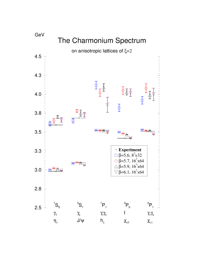
FIG. 1.: Measured at four values of lattice spacings, the charmonium masses are plotted on the top of experimental values (shown as horizontal lines wherever available).

FIG. 2.: The continuum $a_{s}^{2}$ extrapolation of mass differences. The four squares correspond to the four $\beta$ values, 5.6, 5.7, 5.9 and 6.1, at fixed renormalized anisotropy $\xi=2$. The vertical dashed line is there to emphasize the continuum limit. Wherever available, a circle on the dashed line is the observed mass difference in Nature.

FIG. 3.: The continuum $a_{s}^{2}$ extrapolation of mass differences, continued from fig 2.

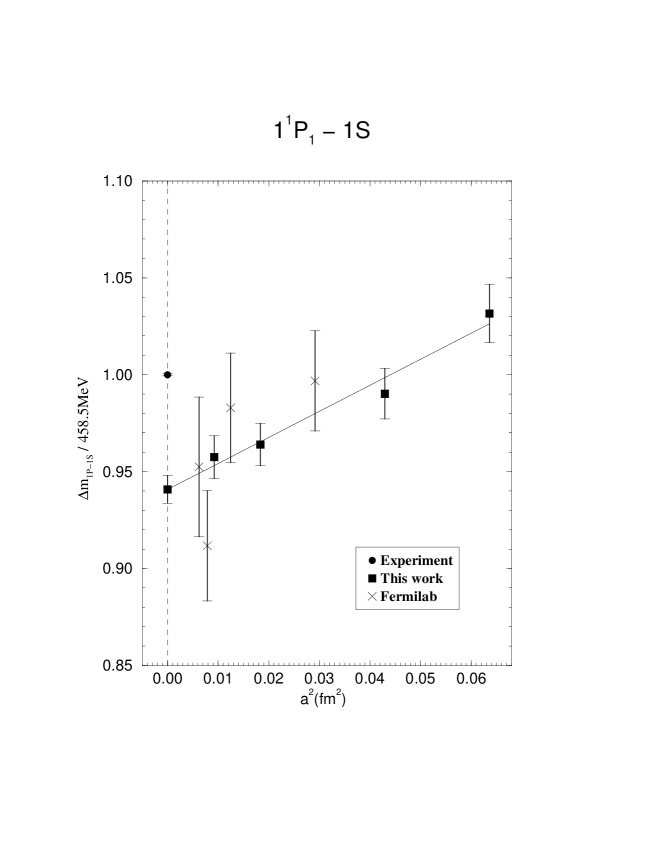
FIG. 4.: The $1^{1}P_{1}-1S$ splitting from several approaches is presented in the form of the ratio $\frac{a_{1^{1}P_{1}-1S}}{a_{r_{0}}}=\frac{\triangle m_{1^{1}P_{1}-1S}}{458.5{\rm MeV}}$. See section V D for more details. The vertical dashed line is to emphasize the continuum limit. The solid line denotes the $a^{2}$ continuum extrapolation of our work.

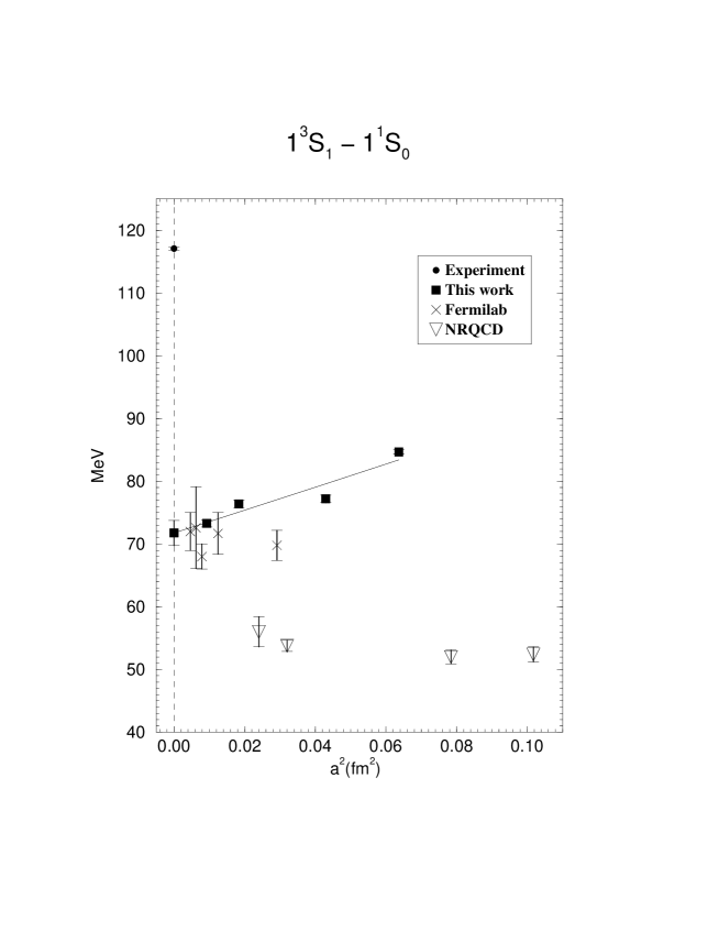
FIG. 5.: The $1^{3}S_{1}-1^{1}S_{0}$ splitting from several approaches. The vertical dashed line is to emphasize the continuum limit. The solid line denotes the $a^{2}$ continuum extrapolation of our work.

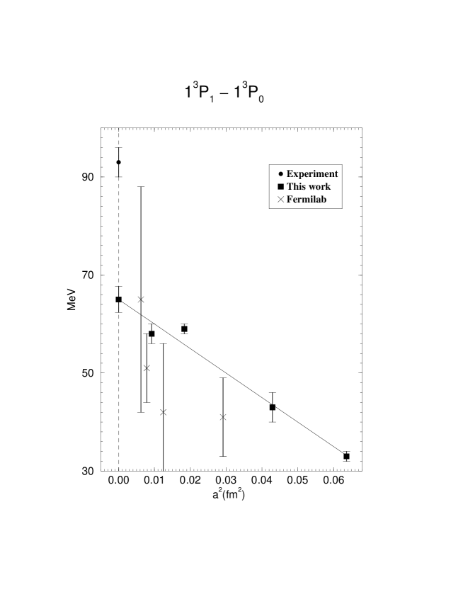
FIG. 6.: The $1^{3}P_{1}-1^{3}P_{0}$ splitting from several approaches. The vertical dashed line is to emphasize the continuum limit. The solid line denotes the $a^{2}$ continuum extrapolation of our work.

REFERENCES

- [1] G. P. Lepage et al., Phys. Rev. D46, 4052 (1992).
- [2] C. Davies eprint hep-ph/9710394.
- [3] H. D. Trottier, Phys. Rev. D55, 6844 (1997).
- [4] N. H. Shakespeare and H. D. Trottier eprint hep-lat/9802038.
- [5] A. X. El-Khadra, A. S. Kronfeld, and P. B. Mackenzie, Phys. Rev. D55, 3933 (1997), eprint hep-lat/9604004.
- [6] T. R. Klassen, Nucl. Phys. B Proc. Suppl. 73, 918 (1999), eprint hep-lat/9809174.
- [7] T. R. Klassen Heavy quarks on anisotropic lattices (unpublished).
- [8] T. R. Klassen, Nucl. Phys. B533, 557 (1998), eprint hep-lat/9803010.
- [9] M. Creutz, Phys. Rev. D21, 2308 (1980).
- [10] A. D. Kennedy and B. J. Pendleton, Phys. Lett. 156B, 393 (1985).
- [11] N. Cabibbo and E. Marinari, Phys. Lett. 119B, 387 (1982).
- [12] R. Sommer, Nucl. Phys. B411, 839 (1994), eprint hep-lat/9310022.
- [13] R. G. Edwards, U. M. Heller, and T. R. Klassen, Nucl. Phys. B517, 377 (1998), eprint hep-lat/9711003.
- [14] R. G. Edwards, U. M. Heller, and T. R. Klassen Unpublished.
- [15] M. R. Hestenes and E. Stiefel, Journal of Research of the National Bureau of Standards Vol. 49, No.6, December 1952 Research Paper 2379.
- [16] W. Press, B. Flannery, S. Teukolsky, and W. Vetterling Numerical Recipes in C: The Art of Scientific Computing.
- [17] C. Caso et al. (Particle Data Group), European Physical Journal C3, 1 (1998).
- [18] J. Simone Private communication on Fermilab results.
- [19] P. Boyle (UKQCD collaboration) eprint hep-lat/9903017.
- [20] D. Chen et al., Nucl. Phys. Proc. Suppl. 73, 898 (1999), eprint hep-lat/9810004.