Edinburgh 2000/12 LTH 455 hep-lat/xxx
Instability in the Molecular Dynamics Step of Hybrid
Monte Carlo in Dynamical Fermion Lattice QCD Simulations

Abstract

We investigate instability and reversibility within Hybrid Monte Carlo simulations using a non-perturbatively improved Wilson action. We demonstrate the onset of instability as tolerance parameters and molecular dynamics step sizes are varied. We compare these findings with theoretical expectations and present limits on simulation parameters within which a stable and reversible algorithm is obtained for physically relevant simulations. Results of optimisation experiments with respect to tolerance parameters are also presented.
Pacs Numbers: 12.38.Gc, 11.15.Ha, 02.70.Lq
Keywords: HMC, Instability, Reversibility, Finite Precision, Higher order integration schemes.

I Introduction

Hybrid Monte Carlo (HMC) [1] remains the most widely used algorithm for lattice QCD computations with dynamical fermions. In such computations, trial configurations are produced by integrating the Hamiltonian equations of motion from an initial configuration for some fictitious molecular dynamics (MD) time $\tau$. Configurations are then accepted or rejected by subjecting the energy change $\delta H$ along a trajectory to a Metropolis [2] accept/reject step.

It has been observed [3, 4] that the equations of motion in the MD evolution of such an algorithm are chaotic in the case of QCD. This implies that rounding errors induced by the use of finite precision in a digital computer may grow exponentially. Such growth can be characterised in terms of the leading Liapunov exponent of the system. Furthermore, it has been shown [4] that the most commonly used MD integration scheme – the leapfrog method – has the potential to become unstable. Instability is a problem for lattice QCD simulations since it results in large energy changes along MD trajectories and hence negligible acceptance rates in the HMC algorithm.

The instability in the leapfrog method has been illustrated in [4] for the case of free field theory where a mechanism has been proposed which could explain the onset of such an instability in lattice QCD. Numerical studies of the latter were carried out on small lattices at a variety of couplings and quark masses. The onset of instability was found to be at smaller step sizes for lighter quark masses.

Edwards, Horváth and Kennedy [4] also investigated an optimisation strategy in which reduced work (and hence accuracy) in the MD calculation was balanced against the resulting reduced acceptance in the Metropolis step. Each MD step requires the iterative solution of a system of linear equations. Since dynamical fermion HMC codes spend a substantial fraction of their execution time performing such solves it it clearly important to investigate whether substantial efficiency gains can be made without introducing undesirable effects such as loss of reversibility in the MD. The investigation [4] was quite preliminary and the errors quoted were quite large. This issue was also investigated on small lattices in [5]. The present paper investigates many of the issues raised in [4] and extends the numerical studies to production-scale lattices.

The paper is organised as follows. In section II we summarise the Hybrid Monte Carlo formalism and give details of the algorithms used. Section III contains a discussion of the effects of numerical roundoff errors on reversibility. In section IV we present results and discussion of our analysis of instability in the MD step. In section V we present the results of an optimisation analysis involving reduced accuracy in the MD step.

Finally, in section VI we summarise our results and conclusions.

II Hybrid Monte Carlo and lattice QCD

A HMC algorithm

Consider a system with canonical coordinates $q$ and action $S(q)$. One wishes to generate configurations $q$ with an equilibrium probability distribution in which the statistical weight of configuration $q$ is proportional to $e^{-S(q)}$.

In Hybrid Monte Carlo, we introduce fictitious momenta $p$ conjugate to $q$ and define a Hamiltonian function $H(q,p)=\frac{p^{2}}{2}+S(q)$.

One may then generate configurations $(q,p)$ distributed according to

$$P(q,p)\ dq\ dp=\frac{1}{Z}e^{-H(q,p)}\ dq\ dp\qquad\mbox{where}\qquad Z=\int dq\ dp\ e^{-H(q,p)}\ .$$ (1)

After the integration over the momenta, we obtain the desired distribution for the coordinates.

Given an initial configuration $(q,p)$, a sequence of configurations is generated by repeated iteration of the following steps:

1. Momentum refreshment:   Draw new fictitious momenta $p$ from a Gaussian distribution with zero mean and unit variance.

2. Molecular dynamics:   Integrate the Hamiltonian equations of motion for some fictitious time trajectory of length $\tau$, from the initial configuration $(q(0),p(0))=(q,p)$ to obtain the trial configuration $(q(\tau),p(\tau))=(q^{\prime},p^{\prime})$.

3. Accept/reject step:   The trial configuration $(q^{\prime},p^{\prime})$ is accepted with probability

   $$P_{\rm acc}(q^{\prime},p^{\prime}\leftarrow q,p)=\min\left(1,e^{-\delta H}\right)$$ (2)

   where

   $$\delta H=H(q^{\prime},p^{\prime})-H(q,p)\ .$$ (3)

   If the trial configuration is rejected the new configuration is $(q,p)$.

B Leap–frog integration

For the HMC algorithm to satisfy detailed balance, the MD is required to be reversible and measure preserving. This can be achieved through the use of symmetric symplectic integration schemes, such as the leapfrog algorithm. In this algorithm, one constructs an approximation ${\cal U}_{3}(\delta\tau)$ to the time evolution operator ${\cal U}(\delta\tau)$ for advancing a phase space vector $(q,p)$ through a step of length $\delta\tau$ in molecular dynamics time. The approximate operator ${\cal U}_{3}(\delta\tau)$ is itself composed of a symmetric combination of the symplectic partial coordinate and momentum update operators ${\cal U}_{\rm q}(\delta\tau)$ and ${\cal U}_{\rm p}(\delta\tau)$ respectively, for example as

$${\cal U}_{3}(\delta\tau)={\cal U}_{\rm p}\left(\frac{\delta\tau}{2}\right){\cal U}_{\rm q}(\delta\tau){\cal U}_{\rm p}\left(\frac{\delta\tau}{2}\right)\ .$$ (4)

The partial update operators are themselves defined as

$${\cal U}_{\rm q}(\delta\tau)\left(q,p\right) = (q+p\delta\tau,p)$$ (5)

$${\cal U}_{\rm p}(\delta\tau)\left(q,p\right) = (q,p+F\delta\tau)$$ (6)

where $F=-\frac{\partial S}{\partial q}$ is the MD force. Due to its symmetric construction, ${\cal U}_{3}(\delta\tau)$ is reversible and, due to the symplectic nature of its component updates, it is area preserving. The process of iteratively acting on an initial phase space vector with ${\cal U}_{3}(\delta\tau)$ is called leapfrog integration. The method is accurate to $O(\delta\tau^{3})$ per time step.

C Higher order integration schemes

The construction of higher order integration schemes (see for example [6, 7]) is recursive, proceeding from the leapfrog scheme. Given an approximate time evolution operator $U_{n+1}(\delta\tau)$ accurate to $O(\delta\tau^{n+1})$ for some even $n$, one can construct the operator

$${\cal U}_{n+3}(\delta\tau)={\cal U}_{n+1}(\delta\tau_{1})^{i}{\cal U}_{n+1}(\delta\tau_{2}){\cal U}_{n+1}(\delta\tau_{1})^{i}$$ (7)

with

$$\delta\tau_{1}=\frac{\delta\tau}{2i-s}$$ (8)

$$\delta\tau_{2}=\frac{\delta\tau}{1-\frac{2i}{s}}$$ (9)

where $i$ is an arbitrary positive integer and $s=(2i)^{1\over{n+2}}$. The step sizes $\delta\tau_{1}$ and $\delta\tau_{2}$ are chosen to cancel truncation orders of $O(\delta\tau^{n+1})$ and symmetry with respect to time ensures that there are no truncation errors of $O(\delta\tau^{n+2})$. Hence such a scheme is accurate to $O(\delta\tau^{n+3})$.

Sexton and Weingarten [8] have considered the general case where the action $S$ can be split into two parts as $S(q)=S_{1}(q)+S_{2}(q)$ and constructed an $O(\delta\tau^{3})$ algorithm in which the coefficient of leading order truncation error term may be decreased. The method is advantageous if evaluating the force corresponding to $S_{1}$ is computationally much cheaper than the force associated with $S_{2}$ (or vice versa). For example, one may take $S_{1}$ to be the gauge action and $S_{2}$ to be some computationally expensive fermion action. The coefficient of the leading error term could then be decreased by performing more gauge update steps than momentum updates.

D Formulation of MD for lattice QCD

The canonical coordinate variables for lattice QCD are the $SU(3)$ link matrices $U_{\mu}(x)$ associated with the link emanating from site $x$ of the lattice and ending on neighbouring site $x+\hat{\mu}$, where $\hat{\mu}$ is a unit vector in one of the Euclidean space–time directions. The conjugate momentum fields $\pi_{\mu}(x)$ are members of the Lie algebra $su(3)$.

In general, one can write the fictitious Hamiltonian for a lattice QCD system with two degenerate flavours of Sheikholeslami-Wohlert (clover) improved [9, 10] fermions as

$$\tilde{H}=\frac{1}{2}\sum_{x,\mu}\pi_{\mu}^{2}+S_{\rm g}(\beta;U)+\phi^{\dagger}\tilde{Q}^{-1}(\kappa,c;U)\phi\ ,$$ (10)

where

$$\tilde{Q}(\kappa,c;U)=M^{\dagger}(\kappa,c;U)M(\kappa,c;U)\,.$$ (11)

Here $M(\kappa,c;U)$ is the clover improved fermion matrix with improvement coefficient $c$, $\phi$ are pseudofermions and $S_{\rm g}(\beta;U)$ is the standard Wilson gauge action

$$S_{\rm g}(\beta;U)=-\frac{\beta}{6}\sum_{\Box}{\rm Re\ Tr\ }U_{\Box}\ .$$ (12)

In (12) the sum is over all elementary plaquettes $U_{\Box}$ on the lattice and $\beta=\frac{6}{g^{2}}$ where $g$ is the bare gauge coupling constant.

In our computations we have employed the technique of even–odd preconditioning which changes the form of $\tilde{Q}$ and $\tilde{H}$ somewhat. Each lattice site is labelled with a parity $p$ which is either even or odd so that any one lattice site has an opposite parity from all of its neighbours. This allows the fermion matrix to be block diagonalised and the Hamiltonian to be re–written as:

$$H=\frac{1}{2}\sum_{x,\mu}\pi^{2}+S_{\rm g}(\beta;U)-2\ {\rm Tr}\ln A_{e}+\phi^{\dagger}_{o}Q^{-1}(\kappa,c;U)\phi_{o}\,.$$ (13)

Here, $A$ is the so called clover term summed over sites of one parity (even in the equation above) and $Q$ is the preconditioned fermion matrix coupling lattice sites of the opposite parity (odd in the equation above) only. Thus $Q$ has half the rank of $\tilde{Q}$. This leads to some memory saving at the additional expense of having to evaluate ${\rm Tr}\ln A$ directly on sites of one parity. The precise formulation of the preconditioned matrices can be found in [11].

We do not expect that splitting the Hamiltonian in this way will change conclusions regarding reversibility and related issues in any significant way. Although there is an extra force term to be computed to integrate the equations of motion, the logarithm of the clover term is computed directly and is independent of the parameters used for the solution of the system of linear equations. Likewise, for the inversion of the clover term, we use a direct method that is not controlled by algorithmic parameters such as a target relative residue. Hence we regard the effects of preconditioning as a minor technicality and shall disregard them for the rest of this paper.

The leapfrog partial update steps for the gauge fields and the momenta are

$${\cal U}_{q}(\delta\tau)\left(U_{\mu}(x),\ \pi_{\mu}(x)\right) = \left(\exp\{i\,\delta\tau\,\pi_{\mu}(x)\}U_{\mu}(x),\,\pi_{\mu}(x)\right)$$ (14)

$${\cal U}_{p}(\delta\tau)(U_{\mu}(x),\ \pi_{\mu}(x)) = \left(U_{\mu}(x),\,\pi_{\mu}(x)+\delta\tau F_{\mu}(x)\right)$$ (15)

where

$$F_{\mu}(x)=F^{\rm g}_{\mu}(x)+F^{\rm f}_{\mu}(x)$$ (16)

and $F^{\rm g}$, $F^{\rm f}$ are the respective gauge and fermionic force contributions,

$$F^{\rm g}_{\mu}(x) = -\frac{\partial S_{\rm g}(U)}{\partial U_{\mu}(x)}$$ (17)

$$F^{\rm f}_{\mu}(x) = \left[Q^{-1}\phi\right]^{\dagger}\frac{\partial Q}{\partial U_{\mu}(x)}\left[Q^{-1}\phi\right]\ .$$ (18)

E Solution of the linear system

Computation of the fermion force requires the quantity

$$X=Q^{-1}\phi$$ (19)

which is obtained via the solution of the linear system

$$QX=\phi\,.$$ (20)

This is normally carried out with a Krylov subspace solver such as the Conjugate Gradients (CG) [12] or the Stabilized BiConjugate Gradients (BiCGStab) [13] algorithm. With the BiCGStab solver, the solution consists of two solves:

$$M^{\dagger}(\kappa,c)Y = \phi$$ (21)

$$M(\kappa,c)X = Y$$ (22)

whereas with CG, one can solve (20) directly. When using CG with a Hermitean positive definite matrix such as $Q$, the solution is guaranteed to converge monotonically. With BiCGStab, one has no such guarantee. Since the condition number of $Q$ is the square of the condition numbers of either $M$ or $M^{\dagger}$, we expect the two stage solution using BiCGStab to be faster on the whole than using one CG solve. As the convergence of BiCGStab can be erratic, it is prudent to restart the solution process for $X$ with CG using, as an initial guess, the solution for $X$ from the previous BiCGStab solve.

The solver residual $r_{i}$ at the $i$-th iteration of a CG solve is defined as

$$r^{\rm Real}_{i}=\|\phi-QX_{i}\|$$ (23)

where $X_{i}$ is the approximate solution at iteration $i$. The relative residual at the $i$-th iteration is then defined as

$$\rho^{\rm Real}_{i}=\frac{r^{\rm Real}_{i}}{\|\phi\|}\ .$$ (24)

In solver algorithms, $r_{i}$ is not usually computed using (23). Instead, $r_{i}$ is generally defined through some three term or coupled two term recurrence relation. We will refer to this latter definition of the residual as $r^{\rm Acc}$, the accumulated residual. The corresponding definition of the relative residual is

$$\rho^{\rm Acc}_{i}=\frac{r^{\rm Acc}_{i}}{\|\phi\|}\ .$$ (25)

These two definitions are equivalent in exact arithmetic. However, computation of the accumulated residual needs only vector additions and scalar multiplications whereas computation of the real residual needs a matrix multiplication and so can differ in finite arithmetic. In our computations we use the accumulated residual. We will denote by $r$ our target relative residual. Hence the iterative process terminates when $\rho^{\rm Acc}_{i}<r$. In the remainder of this paper we refer to $r$ as the solver target residual, or just simply the solver residual.

III Reversibility

Reversibility and area preservation of the Molecular Dynamics step are required for a correct HMC algorithm. The leapfrog algorithm described in section 2, is reversible and area preserving in exact arithmetic. Computations are of necessity carried out in finite precision and exact reversibility is lost. It is therefore important to verify that implementation of the fundamental steps of the algorithm are as close to reversible as it is possible to make them.

Ideally, one would like to establish the least level of precision required such that the accumulation of rounding errors does not introduce a significant bias into the end results of a calculation. At present, it is not possible to give a fully quantitative answer to this question. The accumulation of rounding errors is a complex phenomenon and, since the underlying equations of motion are known to be chaotic, the potential for introducing large uncontrolled errors is great [3, 4]. The best one can do is to ensure that the implementation of each algorithmic component is as close to reversible as practical and that the accumulation of errors grow in the expected way and so remain under control.

We study the reversibility of gauge and momentum update components separately.

A Gauge update

The gauge update involves the process of exponentiating the conjugate momenta on all lattice links [14, 15]. One wishes to verify here that

• the exponentiation of the momenta does produces a suitable unitary matrix;

• the exponentiation of the momenta is reversible in the sense that

  $$\exp(i\pi_{\mu}(x)\delta\tau)=\exp(-i\pi_{\mu}(x)\delta\tau)^{\dagger}\ .$$ (26)

To check these properties, we studied

$$\Delta{\rm Unit} = \max_{x,\mu,a,b}\left|\left(\exp(i\pi_{\mu}(x)\delta\tau)\exp(i\pi_{\mu}(x)\delta\tau)^{\dagger}-1\right)_{ab}\right|$$ (27)

$$\Delta{\rm Rev} = \max_{x,\mu,a,b}\left|\left(\exp(i\pi_{\mu}(x)\delta\tau)-\exp(-i\pi_{\mu}(x)\delta\tau)^{\dagger}\right)_{ab}\right|\ ,$$ (28)

where $x$, $\mu$, $a$ and $b$ are site, direction and colour indices respectively. These observables measure the maximum violations of unitarity and hermiticity on a given lattice.

In tests of the gauge field update reversibility, we used quenched lattices with $V=4^{4}$ sites at $\beta=5.4$. For the MD evolution we used $\tau=1$ and $\delta\tau=\frac{1}{10}$. The maximum values of both $\Delta{\rm Unit}$ and $\Delta{\rm Rev}$ along a molecular dynamics trajectory were found to be

$$\max_{\rm traj}\ \Delta{\rm Unit}=\max_{\rm traj}\Delta{\rm Rev}=0.59604635\times 10^{-7}\approx\frac{1}{2}\epsilon_{SP}\ ,$$ (29)

where $\epsilon_{SP}$ is the single precision unit of least precision. The fact that the maxima of the metrics agree to 8 decimal places may seem surprising at first, but becomes less mysterious when we recall that we are working at the limits of single precision, where the discrete nature of floating point numbers on a computer becomes apparent. Hence, there is only a discrete set of numbers available that the metrics can take of which the figure quoted above is one.

B Momentum update

In the momentum update there are two possible sources of reversibility violation. The first is a lack of associativity in the addition $p(\tau+\delta\tau)=p(\tau)+F(U)\delta\tau$ required in the update step. The second arises in the computation of the force $F$. However, when performing a momentum update forward in time for a step $\delta\tau$ followed immediately by a momentum step backwards in time for $\delta\tau$, (with no gauge field update in between) the gauge fields, and hence the force, should remain unchanged. Thus, reversibility due to lack of associativity in the addition can be isolated.

Consider a test where one starts with a set of fields $(U,\pi,\phi)$. First the momentum fields are updated forward in time for a timestep $\delta\tau$ to produce fields $(U,\pi^{\prime},\phi)$ and then a momentum update is performed backwards in time to produce fields $(U,\pi^{\prime\prime},\phi)$. We use the same value of the force $F$ for both of the updates. One can then define the quantity

$$\Delta\pi^{i}_{\mu}(x)=\pi^{i}_{\mu}(x)^{\prime\prime}-\pi^{i}_{\mu}(x)$$ (30)

as a measure of the reversibility violation incurred by the momentum update step. To improve statistics, one may repeat this several times, in each case using a new set of initial momenta drawn from a Gaussian distribution.

In the numerical tests, we started from some initial gauge field configuration and performed MD in the ordinary sense. Before every momentum update, we performed 100 forward–backward steps with newly drawn momenta in each case. After the test was completed, we restored the original momenta from the end of the last gauge update step and allowed the MD to continue. Thus we obtained an estimate of $\langle\Delta\pi^{i}_{\mu}(x)\rangle$, the average reversibility violation due to lack of associativity in the addition. At the end of the complete trajectory, the resulting data was split into 8 sets, one corresponding to each of the Lie algebra indices $i$. The data in each set was histogrammed to obtain the distribution of the average reversibility violation for each momentum component.

The results of these momentum update tests are shown in figure 1. We show the histograms of all 8 momentum components. The errors on the data points are small and, to aid clarity, are not displayed. The lattice volume used for these tests was $V=4^{3}\times 8$ sites and physical parameters were $\beta=5.2$, $c=0$ and $\kappa=0.1360$. We performed the tests following each gauge field update along a trajectory consisting of 10 timesteps, each of length $\delta\tau=0.1$. We used 500 bins for each momentum component in the histograms. The histogramming process itself was carried out in double precision, allowing us to resolve reversibility violations of $O(10^{-1}\epsilon_{SP})$.

FIG. 1.: Distribution of momentum update reversibility violations obtained by histogramming $\langle\Delta\pi\rangle$. Each plot corresponds to a separate momentum component and $\epsilon_{SP}$ is the single precision unit of least precision.

Figure 1 shows that the distribution of reversibility violations forms a very narrow, apparently symmetric, distribution around $0$ with a width that is of $O(10^{-1}\epsilon_{SP})$. We conclude that the momentum update step in itself is as reversible as it is possible to attain. The apparent symmetry of the distribution may possibly be used to make more general statements about reversibility and area preservation holding stochastically [16].

C Reversibility of the force computation

Since gauge fields are unchanged along a momentum update and computation of the force due to gauge fields is an entirely deterministic process, one expects that the force computation will be reversible. However, the pseudofermion contribution to the force requires solution of a linear equations, so further scrutiny is required.

It has been pointed out [17] that the solution process should be reversible, provided that a time symmetric initial guess vector (such as a zero vector or vector with random components) is used to start the solution process. This makes it tempting to carry out such solves with a large target residue $r$, and hence save on the computational workload. We discuss this further in sections III G and V.

Another commonly used solver strategy is to use the solution from the force computation of the previous momentum update as an initial guess. This, and variants which use a more elaborate extrapolation of previous solutions, may reduce the computational workload but are inherently non-reversible unless the solutions are effectively exact.

D Global Reversibility Violations

Having discussed the sources of reversibility violation at a microscopic level, we now turn to the problem of their global accumulation. Consider an MD trajectory with initial fields $(U,\pi)$ and a set of pseudofermion fields $\phi$. The latter remain unchanged along an MD trajectory. Suppose we perform an MD trajectory forward to obtain fields $(U^{\prime},\pi^{\prime})$, then having reversed the momenta, perform a second (backward) trajectory and a momentum flip to obtain fields $(U^{\prime\prime},\pi^{\prime\prime})$. One may define the following global reversibility violation metrics:

$$\|\Delta\delta U\| = \sqrt{\sum_{x,\mu,a,b}|U^{ab}_{\mu}(x)^{\prime\prime}-U^{ab}_{\mu}(x)|^{2}}\ ,$$ (31)

$$\|\Delta\delta\pi\| = \sqrt{\sum_{x,\mu,i}\left(\pi^{i}_{\mu}(x)^{\prime\prime}-\pi^{i}_{\mu}(x)\right)^{2}}\ ,$$ (32)

$$|\Delta\delta H| = \left|H(U^{\prime\prime},\pi^{\prime\prime},\phi)-H(U,\pi,\phi)\right|\ .$$ (33)

It is also useful to consider these quantities suitably normalised by their respective degrees of freedom:

$$\|\Delta\delta U\|_{\rm d.o.f}=\frac{\|\Delta\delta U\|}{\sqrt{N^{U}_{\rm d.o.f}}}\ ,\qquad\|\Delta\delta\pi\|_{\rm d.o.f}=\frac{\|\Delta\delta\pi\|}{\sqrt{N^{\pi}_{\rm d.o.f}}}\qquad\mbox{and}\qquad|\Delta\delta H|_{\rm d.o.f}=\frac{|\Delta\delta H|}{\sqrt{N^{H}_{\rm d.o.f}}}\,.$$ (34)

Here $N^{U}_{\rm d.o.f}=N^{\pi}_{\rm d.o.f}=4\times 8\times V$ are the respective number of the gauge and momentum degrees of freedom (4 links per site and 8 $SU(3)$ generators) and $N^{H}_{\rm d.o.f}$ is the number of degrees of freedom involved in computing the Hamiltonian H. In the quenched approximation $N^{H}_{\rm d.o.f}=N^{U}_{\rm d.o.f}+N^{\pi}_{\rm d.o.f}$. When dynamical fermions are included, there is an additional factor from the fermions of $N^{f}_{\rm d.o.f}=24\times V$ (3 colour and 4 Dirac complex components per site). In the even–odd preconditioned systems, half of the $N^{f}_{\rm d.o.f}$ degrees of freedom are represented in the pseudofermion vectors and the remainder absorbed into computing ${\rm Tr}\ln A$ on sites of the opposite parity.

We also study $\frac{|\Delta\delta H|}{|\delta H|}$, where

$$\delta H=H(U^{\prime},\pi^{\prime})-H(U,\pi)\,.$$ (35)

This is a measure of the relative error in our energy calculations and is related to the accuracy of the acceptance probability. One would like this relative error to be quite small, certainly no more than a few percent.

E Volume scaling of global reversibility metrics

According to their definitions, $\|\Delta\delta U\|$ and $\|\Delta\delta\pi\|$ should scale as $O(\sqrt{V})$, since the metrics require the summation of $O(V)$ positive definite quantities. We therefore expect that the corresponding normalised (per degree of freedom) metrics should volume-independent. For $|\Delta\delta H|$, the summation involves numbers which are not positive-definite, and one might expect some cancellation. If the numbers are truly random, the cancellations between the terms can be modelled as a random walk and one would expect the sum to scale as $O(\sqrt{V})$. Hence one would expect $|\Delta\delta H|_{\rm d.o.f}$ to be independent of the system volume in a manner similar to the $\|\Delta\delta U\|_{\rm d.o.f}$ and $\|\Delta\delta\pi\|$ metrics.

To satisfy ourselves further that our simulation code is performing as well as can be expected, we carried out reversed trajectories (as described in the definition of the metrics) in the quenched approximation with lattices of different volumes. In each case, we used a single configuration as the starting gauge field for the test and the momentum field was drawn randomly from a heat bath. The trajectory length was $\tau=1$ and the length of the timestep was $\delta\tau=\frac{1}{180}$. We used $\beta=5.4$ and lattices of volume

$$V\in\{4^{4},8^{4},10^{3}\times 16,16^{3}\times 32\}\ .$$ (36)

Results of these tests are shown in figure 2 where the volumes have been normalised by the smallest one ($V_{0}=4^{4}$). We note that the degree of freedom normalised metrics – $\|\Delta\delta U\|_{\rm d.o.f}$, $\|\Delta\delta\pi\|_{\rm d.o.f}$ and $\|\Delta\delta H\|_{\rm d.o.f}$ – are all independent of the volume as expected. We also note that the relative error $\frac{|\Delta\delta H|}{|\delta H|}$ is less than of order $0.1\%$, showing that error in computing the acceptance probability is small.

FIG. 2.: Volume scaling of reversibility metrics, $\|\Delta\delta U\|_{\rm d.o.f}$, $\|\Delta\delta\pi\|_{\rm d.o.f}$, $|\Delta\delta H|_{\rm d.o.f}$ and $\frac{|\Delta\delta H|}{|\delta H|}$. The volumes are normalised by the smallest volume used: $V_{0}=4^{4}$ sites.

F Accumulation of rounding errors in MD time

It has been noted by several authors that the MD equations of motion are chaotic [3, 4] and so effects of roundoff error are expected to grow exponentially with MD time along a trajectory. In particular, if one were to carry out reversed trajectory tests, as described in the definition of the metrics $\|\Delta\delta U\|$ and $\|\Delta\delta\pi\|$, these would be expected to exhibit the leading behaviour

$$\|\Delta\delta U\|\propto e^{\nu_{U}\tau}\qquad\mbox{and}\qquad\|\Delta\delta\pi\|\propto e^{\nu_{\pi}\tau}$$ (37)

as a function of the MD trajectory length $\tau$. We use this as an operational definition of the effective leading Liapunov exponents $\nu_{U}$ and $\nu_{\pi}$. In our computations we measured only $\nu_{U}$ and, hence, in future discussion we shall drop the subscript $U$ and refer to it simply as $\nu$. We shall also refer to $\nu$ simply as the Liapunov exponent.

The authors of [3, 4, 5] all found positive values for the Liapunov exponents in their studies. In particular it was shown in [4] that as the solver target residue $r$ and MD step–size $\delta\tau$ were made smaller, the Liapunov exponents appeared to plateau, indicating that chaos was present in the underlying continuum equations of motion for the system and not just a feature of the numerical integration scheme.

For the leading Liapunov exponent $\nu$, the authors of [4] found that this plateau came to an end at $\delta\tau\approx 0.6$ in the quenched approximation and in the case of dynamical fermion simulations with sufficiently heavy quarks. Beyond this step size, the effective exponent exhibited growth. However, in the case of light quarks, this growth was found to set in significantly earlier, at $\delta\tau\approx 0.08$. This sudden growth in Liapunov exponents could signal the onset of instability in the MD. The subject of integrator instabilities will be taken up in section IV.

The authors of [4] also studied the behaviour of the Liapunov exponents as a function of the MD solver target residue $r$. They investigated the effects of increasing $r$ (using a time symmetric start) as a possible means of improving computational efficiency. Their data indicated a sudden growth in Liapunov exponent as $r$ is increased beyond a critical value. The data covered a limited range of $r$, and had large statistical errors. However, the sudden apparent growth of the Liapunov exponent coincides with a dramatic drop in acceptance rate, suggesting again that the integrator has become unstable.

G Tuning the solver target residual

The results of [4] motivated us to measure the Liapunov exponents of our simulations while varying the target residue of a comparatively large volume system, with comparatively light quarks such as those in current production runs.

For the determination of Liapunov exponents, we used 10 configurations taken from one of our large data sets. The lattice volume used was $V=16^{3}\times 32$ and the physical parameters were $\beta=5.2$, $c=2.0171$ and $\kappa=0.1355$. The value of the clover coefficient was calculated using the formula determined by the Alpha collaboration [10]. These parameters correspond to pseudoscalar to vector mass ratio of $\frac{m_{\pi}}{m_{\rho}}\approx 0.6$ [18] and a lattice spacing of $a=0.097\mathop{\rm fm}$ [18] where the physical lattice spacing has been determined using the observable $r_{0}$[19]. By current standards, the dynamical fermions are relatively light.

Using the 10 starting configurations, for a given value of $r$ we carried out reversed MD trajectories of varying length $\tau$ with a constant step–size of $\delta\tau=\frac{1}{180}$. This value for $\delta\tau$ was the one used in the production of the dataset from which our 10 sample configurations were taken. Our MD solver strategy was to employ a two stage BiCGStab solution to compute the quantity $X$ of (19) followed by a restarted CG solution. Hence the target residue used was the accumulated target residue for the CG solver as described in section II E. The target residues used ranged from $r=10^{-7}$ to $r=10^{-4}$. The smallest of these is near the limit of what may be achieved in a single precision (32bit) computation.

In each test we measured $\|\Delta\delta U\|$, $|\delta H|$ and $N_{\rm iters}$, where $N_{\rm iters}$ was the total number of solver iterations carried out in both the BiCGStab and CG solves averaged over the forward and reverse trajectories. For each combination of parameters, we also calculated the Metropolis acceptance probability $P_{\rm acc}$.

To evaluate the savings (or losses) in computational cost we defined the cost metric

$$\mbox{Cost}=\frac{N_{\rm iters}}{P_{\rm acc}}\ .$$ (38)

This heuristic measure reflects the fact that a large number of iterations along an MD trajectory implies high computational cost, as does a low Metropolis acceptance rate. We note that an absolute measure of cost should also take into account the autocorrelation time of the ensemble produced by an HMC computation. Since we are unable to control or measure this quantity on a sample of 10 configurations, we disregard autocorrelation effects in this study where we are interested in the relative cost with different choices of simulation parameters.

Figure 3 shows fits used to extract the (effective) Liapunov exponents. The system is clearly chaotic as $\ln\|\Delta\delta U\|$ has a significant positive slope as a function of $\tau$. Even with only 10 configurations, the signal for the Liapunov exponents is good except for the cases when $r=5\times 10^{-6}$ and when $r=10^{-5}$. The data for these latter parameter values seem to show a marked break at $\tau\approx 0.6$ and indeed, it was not possible to establish a consistent value of the Liapunov exponent for these two values of $r$.

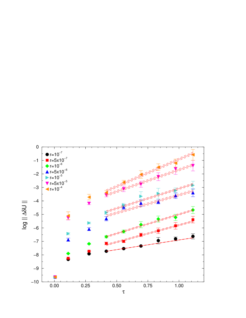
FIG. 3.: Fits for the Liapunov Exponent $\nu$.

In figure 4 we show $\langle\delta H\rangle$, the energy change along an MD trajectory averaged over 10 configurations as a function of trajectory length $\tau$. One can clearly distinguish three different types of behaviour for $\langle\delta H\rangle$ depending on the target MD residual $r$. For values of $r<5\times 10^{-6}$, $\langle\delta H\rangle$ shows an oscillatory behaviour with $\tau$, whereas for $r>10^{-5}$ $\langle\delta H\rangle$ diverges with increasing $\tau$, resulting in a corresponding exponential drop in acceptance probability. It is interesting to note that this change in the behaviour of $\delta H$ occurs at the value of $r$ where the data in figure 3 also show a change.

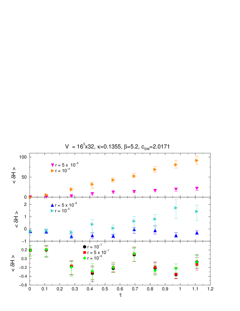
FIG. 4.: $\langle\delta H\rangle$ as a function of $\delta\tau$ for various values of $r$.

A summary of results for tuning the solver residue is shown in figure 5. The bottom panel shows the Liapunov exponents $\nu$. For each value of $r$ we made several determinations of $\nu$ by fitting to different ranges of $\tau$ in figure 3. We note that the results of these different fits are consistent with each other except for the values of $r=5\times 10^{-6}$ and $r=10^{-5}$ corresponding to the “break” evident in figure 3.

We note that, overall, the Liapunov exponents appear to show a slow growth with $r$. There is no evidence of a plateau as $r$ is reduced to $r=10^{-7}$. This implies that this manifestation of chaos in the system is not due to the underlying equations of motion, but to the integrator. The behaviour of the exponents near $r=10^{-5}$ may perhaps be interpreted as the effect of the integrator changing from being stable to being unstable.

The second panel in figure 5 shows the average acceptance rate $\langle P_{\rm acc}\rangle$ for trajectories of length $\tau\approx 1$. The acceptance shows a rapid drop for $r>10^{-5}$, which is due to the divergent behaviour of $\delta H$ for values of $r$ in this region. The rapid drop in acceptance rate results in a huge growth in the cost of the algorithm as shown in the third panel of figure 5 where we display the cost metric (38) normalised by its value for the simulation with $r=10^{-7}$.

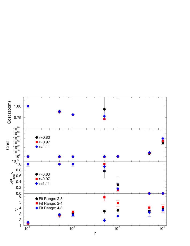
FIG. 5.: Liapunov exponents, acceptance rate and cost as a function of $r$.

In the top panel of figure 5 we show an enlarged view of the cost function for values of $r<10^{-5}$. The cost metrics for values of $r\geq 10^{-5}$ are too large to fit onto this enlarged plot. We note that the normalised cost has a shallow minimum when $r=5\times 10^{-6}$ however at this minimum value the normalised cost has a value of about 0.75 implying a saving of only about $25\%$.

IV Instability in the MD integration

The behaviour of the energy change $\delta H$, from oscillatory to divergent, is reminiscent of a known instability in the leapfrog algorithm when applied to the integration of the equations of motion for the simple harmonic oscillator. In this section, we review the simple harmonic oscillator analysis of [4] and compare expectations for interacting theories with our numerical results.

A Harmonic Oscillator

In what follows we use the notation of  [4]. Consider a single oscillator with coordinate $\phi$. The corresponding Hamiltonian function is

$$H={1\over 2}\left(\pi^{2}+\omega^{2}\phi^{2}\right)\ ,$$ (39)

where $\omega$ is the angular frequency of the oscillator and $\pi$ is the corresponding fictitious momentum.

The leapfrog update for the coordinate and momentum may be written in the form of a matrix ${\mathcal{U}}_{3}(\delta\tau)$ acting on the phase space vector $(\phi,\pi)$

$${\mathcal{U}}_{3}(\delta\tau)=\left(\begin{array}[]{cc}1-\frac{1}{2}\omega^{2}\delta\tau^{2}&\delta\tau\\ -\omega^{2}\delta\tau+\frac{1}{4}\omega^{4}\delta\tau^{3}&1-\frac{1}{2}\omega^{2}\delta\tau^{2}\end{array}\right)\,.$$ (40)

The update matrix ${\cal U}_{3}$ can be parameterised as

$${\mathcal{U}}_{3}(\delta\tau)=\left(\begin{array}[]{cc}\cos[\kappa(\delta\tau)\delta\tau]&\displaystyle\frac{\sin[\kappa(\delta\tau)\delta\tau]}{\rho(\delta\tau)}\\ -\rho(\delta\tau)\sin[\kappa(\delta\tau)\delta\tau]&\cos[\kappa(\delta\tau)\delta\tau]\end{array}\right)$$ (41)

where

$$\kappa(\delta\tau) = \frac{\cos^{-1}(1-\frac{1}{2}\omega^{2}\delta\tau^{2})}{\delta\tau}$$ (42)

$$\rho(\delta\tau) = \omega\sqrt{1-\frac{1}{4}\omega^{2}\delta\tau^{2}}\ .$$ (43)

Evolution over a whole trajectory of length $\tau$ is then given by

$${\mathcal{U}}_{3}(\tau)=\left(\begin{array}[]{cc}\cos[\kappa(\delta\tau)\tau]&\displaystyle\frac{\sin[\kappa(\delta\tau)\tau]}{\rho(\delta\tau)}\\ -\rho(\delta\tau)\sin[\kappa(\delta\tau)\tau]&\cos[\kappa(\delta\tau)\tau]\end{array}\right)\ .$$ (44)

The nature of the instability in the leapfrog scheme may be illustrated by examining the phase space trajectories in this system. The initial phase space vector for an oscillator released from amplitude $A$ is $(\phi(0),\pi(0))=(A,0)$. From (44), the phase space vector at time $\tau$ is then given by

$$\left(\begin{array}[]{c}\phi(\tau)\\ \pi(\tau)\end{array}\right)=\left(\begin{array}[]{c}A\cos[\kappa(\delta\tau)\tau]\\ -A\rho(\delta\tau)\sin[\kappa(\delta\tau)\tau]\end{array}\right)\,.$$ (45)

The phase space orbits therefore satisfy

$$\frac{\phi^{2}(\tau)}{A^{2}}+\frac{\pi^{2}(\tau)}{A^{2}\rho^{2}(\delta\tau)}=1\,.$$ (46)

It can then be seen from (43) and (46) that for $\omega\delta\tau<2$ the phase space trajectories are elliptical, whereas for $\omega\delta\tau>2$ they are hyperbolic. The instability at $\omega\delta\tau=2$ is the abrupt transition from one class of phase space trajectories to another.

The change in energy

$$\delta H=H(\phi(\tau),\pi(\tau))-H(\phi(0),\pi(0))$$ (47)

may also be computed. Using the same initial conditions,

$$\delta H=-\frac{1}{8}\omega^{4}A^{2}\delta\tau^{2}\sin^{2}[\kappa(\delta\tau)\tau]\,.$$ (48)

When $\omega\delta\tau<2$, $\kappa(\delta\tau)$ is real and so $\delta H$ oscillates with increasing $\tau$, in a manner similar to that observed in the bottom panel of figure 4. However, when $\omega\delta\tau>2$, $\kappa(\delta\tau)$ becomes purely imaginary causing $\delta H$ to diverge as ${\rm sinh}^{2}[\kappa(\delta\tau)\tau]$ in a manner similar to that seen in the top panel of figure 4.

B Generalised treatment of instabilities

We now present a more general method of finding instabilities in the leapfrog algorithm and in higher order schemes of the type discussed in [6, 7] (see section II C) when applied to the case of a harmonic oscillator.

Consider an initial phase space vector $(\phi,\pi)$ of the harmonic oscillator. This is to be evolved through phase space by the leapfrog matrix ${\mathcal{U}}_{3}(\delta\tau)$ of (40). The area preservation property of the integrator implies that $\det({\mathcal{U}}_{3}(\delta\tau))=1$. All components of ${\mathcal{U}}_{3}(\delta\tau)$ are real, implying that ${\rm Tr}\ {\mathcal{U}}_{3}$ is also real.

If

$$\lambda_{1}=u_{1}+iv_{1}\qquad\mbox{and}\qquad\lambda_{2}=u_{2}+iv_{2}$$ (49)

are the two eigenvalues of ${\mathcal{U}}_{3}(\delta\tau)$, the previous conditions on the trace and the determinant (area preservation) can then be shown to imply that

$$v_{1}=-v_{2}\quad\hbox{and}\quad u_{1}v_{2}+u_{2}v_{1}=0\ .$$ (50)

We conclude that either:

1. $u_{1}=u_{2}$   or

2. $v_{1}=v_{2}=0$

In case 1), the determinant condition ($\lambda_{1}\lambda_{2}=1$) implies that $u_{1}^{2}+v_{1}^{2}=1$. The eigenvalues have magnitude unity: $\lambda_{1,2}=e^{\pm i\theta}$ with $\theta$ real, and the update matrices ${\mathcal{U}}_{3}(\delta\tau)$ and ${\mathcal{U}}_{3}(\tau)$ ($={\mathcal{U}}_{3}^{N_{\rm MD}}(\delta\tau)$) give stable elliptical trajectories in phase space.

In case 2), by the same condition on the determinant, we have that $\lambda_{1}=\eta$ and $\lambda_{2}=\frac{1}{\eta}$ for some real $\eta\geq 1$. On raising $\lambda_{1}$ or $\lambda_{2}$ to the power $N_{\rm MD}$, one of the eigenvalues of ${\mathcal{U}}_{3}(\tau)$ will show an exponential divergence with $N_{\rm MD}$. This implies unstable behaviour in the integrator.

The condition for the onset of instability is that the eigenvalues change from being complex to real. This information can be deduced from the discriminant of the characteristic polynomial of the update matrix ${\mathcal{U}}_{3}(\delta\tau)$. The onset of instability occurs as the discriminant changes sign from negative to positive.

For the leapfrog method, the discriminant is given by

$$D_{3}=(\omega\delta\tau)^{2}(\omega\delta\tau-2)(\omega\delta\tau+2)\,.$$ (51)

We note that for $0<\omega\delta\tau<2$, the discriminant is negative indicating a stable integrator, whereas for $\omega\delta\tau>2$ the discriminant is positive implying an unstable integrator in line with the previous discussion.

C Instability in Higher Order Schemes

Consider the 5th order scheme of Campostrini and Rossi [6]. This can be constructed from three leapfrog integration steps as

$${\mathcal{U}}_{5}(\delta\tau)={\mathcal{U}}_{3}(\delta\tau_{1}){\mathcal{U}}_{3}(\delta\tau_{2}){\mathcal{U}}_{3}(\delta\tau_{1})$$ (52)

with $\delta\tau_{1}=\frac{\delta\tau}{2-2^{1/3}}$ and $\delta\tau_{2}=-\frac{2^{1/3}\delta\tau}{2-2^{1/3}}$. This corresponds to $n=3$ and $i=1$ in (8) and (9).

The discriminant $D_{5}$ is a 12th order polynomial in $\omega\delta\tau$ which can easily be found using an algebraic package such as Maple. It is not reproduced here but plotted in figure 6. The nonnegative roots of the $D_{5}=0$ are found to be

$$\omega\delta\tau\in\{0,\sqrt{12-6\sqrt[3]{4}}\}\,.$$ (53)

To three decimal places, the positive root is at $1.573$. The discriminant is negative for $0<\omega\delta\tau<1.573$ indicating stable behaviour and is positive for $\omega\delta\tau>1.573$ for the region where the integrator is unstable.

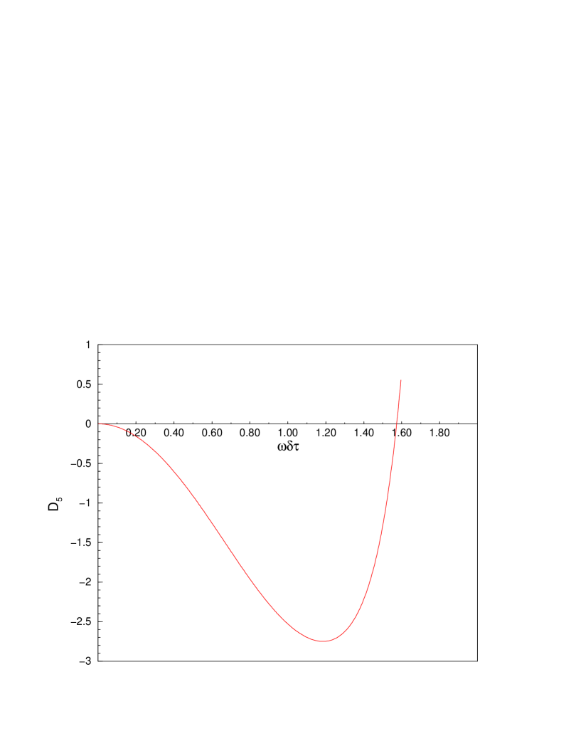
FIG. 6.: The discriminant $D_{5}$ of characteristic polynomial of the 5th-order Campostrini-Rossi update matrix ${\mathcal{U}}_{5}(\delta\tau)$.

It is interesting to note that, for the central leapfrog update matrix ${\mathcal{U}}_{3}(\delta\tau_{2})$ in the 5th order scheme to become unstable on its own, requires that $\omega\delta\tau_{2}=2$. This implies that this central step should go unstable when

$$\omega\delta\tau=2\frac{\left(2-2^{1/3}\right)}{2^{1/3}}\approx 1.175\ .$$ (54)

This suggests that, although the central update itself becomes unstable at $\delta\tau=1.175$, the other two updates in the scheme stabilize the system until $\delta\tau\approx 1.57$.

Following a similar calculation, it can be shown that the discriminant $D_{7}$ of the characteristic polynomial for the update matrix of the 7th order scheme ($n=5$, $i=1$) has roots at

$$\omega\delta\tau\in\{0,1.595,1.822,1.869\}$$ (55)

with $D_{7}$ being negative in the intervals $D_{7}\in(0,1.595)$ and $D_{7}\in(1.822,1.869)$ indicating two domains of stability. The discriminant is positive for $D_{7}\in(1.592,1.822)$ and for $D_{7}>1.869$. For the longest constituent 5th order update to go unstable in this scheme requires that $\omega\delta\tau>1.166$.

Hence we see that, for the case of the simple harmonic oscillator at least, higher order integration schemes do not help cure the problem of instabilities. Indeed, they become unstable at even smaller values of $\omega\delta\tau$ than the simplest leapfrog method.

D Hypothesis for interacting field theories

Edwards, Horváth and Kennedy [4] advanced the hypothesis that, since the high frequency modes of an asymptotically free field theory can be considered as a collection of weakly coupled oscillator modes, the instability just described in the harmonic oscillator system will also be present for interacting field theories. The onset of the instability will be caused by the mode with highest frequency $\omega_{\rm max}$, when $\omega_{\rm max}\delta\tau=2$. For a single oscillator mode, the onset of instability is abrupt. In the case of an interacting theory, one would expect the effects of the interactions to smooth out this transition.

It is argued in [4] that the instability in lattice QCD with dynamical fermions can be likened to that of a collection of oscillator modes of the sort just described. When applying leapfrog integration to this system, the rôle of $\omega^{2}\phi$ in the harmonic oscillator example is played by the MD force $F_{\mu}(x)$. This force can be written as a sum of contributions from the gauge and fermionic pieces of the action as $F_{\mu}(x)=F^{\rm g}_{\mu}(x)+F^{\rm f}_{\mu}(x)$, where the subscripts $g$ and $f$ indicate the gauge and fermionic components of the force respectively.

The fermion force is expected to be proportional to $m_{f}^{\alpha}$, where $m_{f}$ is the mass of the lightest species of dynamical fermion and $\alpha$ is some negative parameter. In the case of Wilson (and Clover) fermions the mass in lattice units is defined as

$$am_{f}=\frac{1}{2}\left(\frac{1}{\kappa}-\frac{1}{\kappa_{c}}\right)$$ (56)

where $\kappa$ now stands for the Wilson hopping parameter, and $\kappa_{c}$ is the critical value corresponding to $m_{f}=0$. It is argued that the highest frequency mode (with frequency $\omega_{\rm max}$) is proportional to the fermion force which, in turn, is expected to be proportional to $m_{f}^{\alpha}$, and thus as $\kappa\rightarrow\kappa_{c}$ ($m_{f}\rightarrow 0$), the fermion force will diverge and hence the critical value of $\delta\tau$ will decrease. In the following, we evaluate numerical evidence for the validity of this hypothesis.

E Studies of the force

The forces used in the momentum update belong to the Lie algebra $su(3)$. We define the 2–norm $\|F\|$ in the same manner as for $\|\Delta\delta\pi\|$:

$$\|F\|=\sqrt{\sum_{x,\mu,i}\left(F^{i}_{\mu}(x)\right)^{2}}\ .$$ (57)

Again, we can define the 2–norm suitably normalised by the relevant degrees of freedom:

$$\|F_{g}\|_{\rm d.o.f}=\frac{\|F_{g}\|}{\sqrt{N^{U}_{\rm d.o.f}}}\qquad\mbox{and}\qquad\|F_{f}\|_{\rm d.o.f}=\frac{\|F_{f}\|}{\sqrt{N^{f}_{\rm d.o.f}}}$$ (58)

where the subscripts $g$ and $f$ indicate gauge and fermionic forces respectively.

We can also define an $\infty$–norm for the forces:

$$\|F\|_{\infty}=\max_{x,\mu,i}\left|F^{i}_{\mu}(x)\right|\ .$$ (59)

The $\infty$–norm then is the force component with the maximum magnitude over the lattice and so can be likened to the force mode with the highest frequency, proportional to $\omega^{2}_{\rm max}$, in the analogous collection of weakly coupled harmonic oscillators. The (degree of freedom) averaged 2–norm on the other hand can be likened to the average frequency–squared of the analogous set of harmonic oscillators.

In our studies we computed the magnitude of the forces at all timesteps of an MD trajectory starting from a single gauge configuration chosen from the same 10 configurations described in section III G (with volume lattice $V=16^{3}\times 32$ sites, and production parameters $\beta=5.2$, $c=2.0171$, $\kappa=0.1355$).

In the first set of tests, we attempted to investigate how the fermion force behaves with the quark mass. We performed MD trajectories consisting of $N_{MD}=175$ steps of length $\delta\tau=\frac{1}{180}$ for several values of the hopping parameter $\kappa$. We measured the norms of the gauge and fermion forces on each timestep. The MD solver target residue was set at $r=10^{-6}$. Error bars for the average value of the force were computed by bootstrapping the 175 samples.

It could be argued that a configuration that has been produced in an ensemble equilibrated at some value of $\kappa$, will have very small statistical weight at a different value of $\kappa$. However, our aim was not to study equilibrium properties of the ensemble, but to test the properties of algorithm components as a function of the external parameter $\kappa$.

The average value of $\kappa_{c}$, the critical value of $\kappa$ corresponding to massless fermions, is known from separate spectroscopy studies for the ensemble from which the configurations were drawn. It is approximately $0.1363$ [18]. Thus, we were able to associate a value of the lattice fermion mass $am_{f}$ with every value of $\kappa$ used in our tests through the formula:

$$am_{f}=\frac{1}{2}\left(\frac{1}{\kappa}-\frac{1}{\kappa_{c}}\right)\ .$$ (60)

Since we expect the fermion mass to vary in some inverse relation to the norm of the force [4], we attempted to fit the results of our tests with the form

$$F=A(am_{f})^{\alpha}=A\left(\frac{1}{2\kappa}-\frac{1}{2\kappa_{c}}\right)^{\alpha}\ ,$$ (61)

where the parameters of the fit were $A$, $\kappa_{c}$ and $\alpha$.

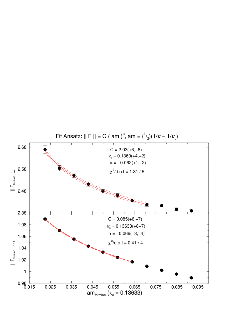
FIG. 7.: Fits to the fermion force as a function of $am_{f}$ using the fitting hypothesis of (61).

Results of this test are shown in figure 7. We show both the fits made to the $\infty$–norm and the (degree of freedom) averaged 2–norm of the force. We can see that good fits can be made, which reproduce $\kappa_{c}$ from the spectroscopic studies and that $\alpha$ is negative indicating that the magnitudes of the norms do indeed vary in an inverse manner with the fermion mass. The fact that the value of $\kappa_{c}$ is well reproduced and that $\alpha$ is negative in sign both lend support to the hypothesis of [4].

F Dependence on $\delta\tau$ and $\kappa$

To investigate further the onset of instability, we computed the averaged forces and $\delta H$ along an MD trajectory using the same starting configurations as before. However, this time we varied the MD step size $\delta\tau$. The number of steps taken along the trajectory was adjusted to keep the trajectory length constant at $\tau=175/180$. The results are plotted in figure 8. From the growth of $\delta H$ evident in the plot, one can see that the instability sets in between $\delta\tau=0.0105$ and $\delta\tau=0.0110$. We can also see that the rapid growth of $\delta H$ is accompanied by a growth in the fermionic forces in the system (in both norms) and that the $\infty$–norm of the force appears to grow more rapidly than the degree of freedom averaged 2–norm. This latter behaviour suggests that the onset of instability is driven by a few unstable fermion modes, again in line with the above hypothesis.

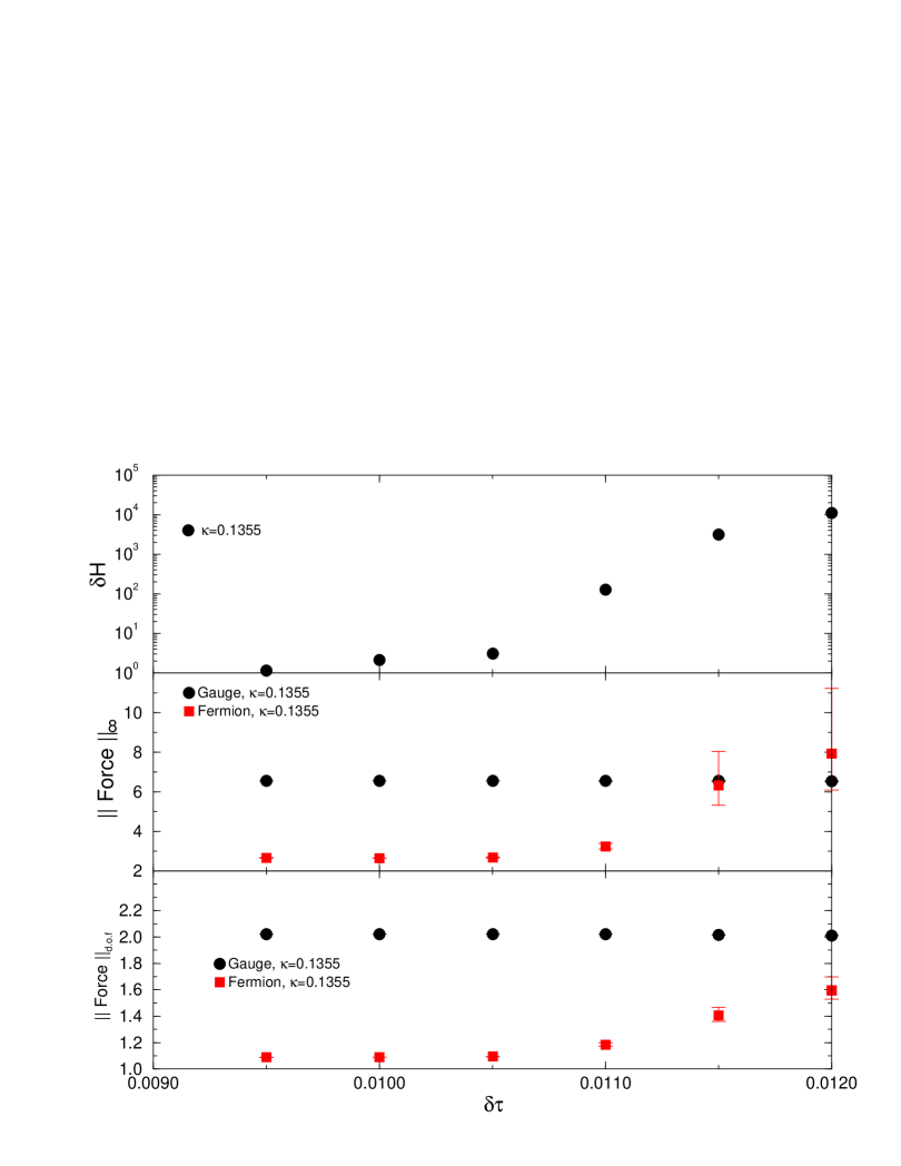
FIG. 8.: The 2–norm and the $\infty$–norm of the average gauge and fermionic components of the MD force along an MD trajectory plotted against the MD stepsize $\delta\tau$. The corresponding behaviour of the energy change $\delta H$ along a trajectory is shown in the top graph.

In a further investigation of the MD forces, we carried out MD trajectories using the same initial gauge configuration as before, this time varying $\kappa$ for two separate values of the step size. The values of the step size were $\delta\tau=0.010$ and $\delta\tau=0.012$ corresponding to stable and unstable MD at $\kappa=0.1355$ respectively, as discussed above.

We show the $\infty$–norms of the gauge and fermion forces in figure 9. This shows that the simulation which was unstable at $\kappa=0.1355$ has become stable as $\kappa$ is reduced. Once again this seems in line with the hypothesis that the onset of the instability is a function of the combination of the fermionic forces (controlled by $\kappa$) and the stepsize $\delta\tau$. Recall that the relevant parameter for the SHO was $\omega\delta\tau$.

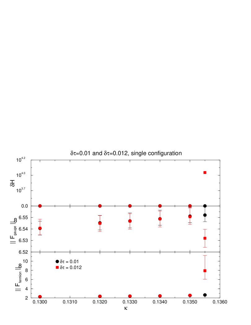
FIG. 9.: The $\infty$–norms of the gauge and fermionic forces, and $\delta H$ against $\kappa$.

Overall, our studies of the MD forces lend support to the hypothesis that the instability is driven by the $F\delta\tau$ term in the momentum update step of the leapfrog algorithm. Since the fermionic force diverges in some inverse relation with the fermion mass, we expect the maximum safe stepsize $\delta\tau$ to decrease as the fermion mass is decreased ($\kappa$ is increased). Also, having observed a faster rise in the $\infty$–norm of the fermionic force than in the degree of freedom averaged 2–norm, we infer that the instability is driven by a comparatively small number of unstable fermionic modes.

V Tuning the stepsize and the solver residue

The above conjecture, if correct, can serve to explain the tuning results described in section III G. By increasing the solver residue $r$, we are modifying the fermionic force which could then drive the MD integrator unstable. In order to investigate these possibilities, we have carried out a second tuning exercise this, time varying both the step size $\delta\tau$ and the solver target residue $r$.

We used the 10 configurations used when tuning $r$ alone in section III G. Since at this point we were not computing Liapunov exponents, our tests consisted of single MD trajectories in one direction only. For each value of $\delta\tau$, we chose the number of steps along the trajectory so as to maintain a constant trajectory length of $\tau=175/180$. We also carried out a test with a target residue of $r=10^{-9}$ using double precision (64bit) floating point numbers, whereas all other tests used single precision. For each combination of algorithmic parameters, we measured the energy change $\delta H$, the corresponding acceptance probability $P_{\rm acc}$ and the cost function of (38).

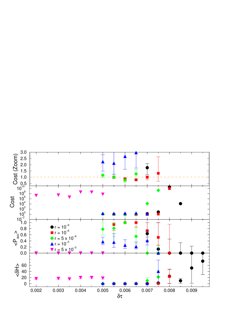
FIG. 10.: The average energy change $\langle\delta H\rangle$, acceptance probability $\langle P_{\rm acc}\rangle$ and cost function for the second tuning study, plotted against step–size $\delta\tau$ for several values of the solver target residue $r$. The cost function is normalised by its value when $\delta\tau=0.0055$, and $r=10^{-6}$.

The results of this tuning exercise are shown in figure 10. First we see in the bottom panel ($r=10^{-9}$ symbols) that using double precision does not alleviate the problem of instability. The calculation in double precision appears to become unstable at a similar value of the step size as does that in single precision. Second, we see from the data for $r=5\times 10^{-5}$ that, if the solver target residue is too large, one cannot achieve values of $\delta H$ of $O(1)$, even if $\delta\tau$ is made very small.

For our simulations, we are able to achieve non–zero acceptance rates when $\delta\tau<0.0075$ and when $r\leq 10^{-5}$. For parameter values smaller than these, we can attempt to tune our simulation for maximum performance. The top two panels of figure 10 show the variation of the cost function. In this case, the cost function is normalised by its value when $r=10^{-6}$ and $\delta\tau=0.0055$. These were the parameters used in the production of the dataset from which the configurations were taken. We see that either by tuning the solver residue $r$ or the MD step size $\delta\tau$, the maximum gain we could make in the cost function is about 25%.

VI Conclusions and Discussion

A Stability

We have shown that, for the physical parameters used in our production simulations, the molecular dynamics integrator used becomes unstable at $\delta\tau\approx 0.01$ for all studied values of $r$, and also for any realistic value of $\delta\tau$ when $r$ was increased above $r\approx O(10^{-5})$. We identify this instability with the one studied in free field theory for the frequency–step-size combination $\omega_{\rm max}\delta\tau=2$. We have studied numerically the fermion force and found that its behaviour is not inconsistent with the hypothesis of [4] (motivated by free field theory) that the force should grow large as $\kappa\rightarrow\kappa_{c}$. We suppose that a critical value exists for $F\delta\tau$ when the leapfrog integrator becomes unstable.

Reducing the value of the MD residual results in an increasingly inaccurate force calculation. If as a result $F$ is too large, one may need an extremely small step-size to keep the integrator stable. We found that, for $r=5\times 10^{-5}$ at our parameters, one would need a step-size much smaller than $\delta\tau=0.001$. (c.f. figure 10).

On the safe side of these limits, one may attempt to tune the algorithm. However, our studies show that on this volume and with these physical parameters, tuning $\delta\tau$ and/or $r$ is unlikely to produce significant performance gains. We note that it appears entirely safe to carry out computations in single precision in the safer region of parameter space. However, as $\kappa\rightarrow\kappa_{c}$, it may be that the upper limit on $r$ decreases beyond the limit of single precision. Alternatively, as the condition number of the fermion matrix increases with increasing $\kappa$, the number of iterations in the solver for fixed $r$ will increase. This may cause rounding errors to accumulate so that the target residual $r$ may not be reached. However, in this latter case, it is only the solve itself that needs to be done in double precision, or restarted in single precision.

B Higher order integration Schemes

We have demonstrated that, at least for the case of a simple harmonic oscillator, the 5th and 7th order schemes of [6, 7] are not immune to instabilities. We expect that this situation will persist for even higher order schemes of this sort. The source of the problem is that, at the bottom level, these schemes are constructed out of simple leapfrog updates. For any given step–size $\delta\tau$ in an integration scheme of order $n+3$, there will always be a sub update of order $n+1$ which will have a stepsize $\delta\tau_{2}>\delta\tau$. This sub–update, or one of its constituent sub–updates, may eventually drive the whole integration scheme unstable, although the other sub-updates may act as a stabilizing factor at first. We note that, in our harmonic oscillator examples, the smallest positive critical value of $\omega\delta\tau$ was always smaller for the higher order integrators than for the leapfrog, indicating that the instability problem is actually worse for the higher order methods.

As the source of the instability appears to come from the fermionic part of the force, we anticipate that a scheme of the type advocated in [8] would not assist avoiding the instability either, as it attempts to improve the truncation error by performing more gauge updates. While this may drive down the truncation error, it does nothing about the problem in the fermionic update.

C Reversibility

Reversibility itself seems not to be strongly affected by changing $r$. The Liapunov exponents of the system seem to show a slow rise before the instability sets in. In the region of transition from stability to instability, the Liapunov exponents are difficult to determine. One might speculate that this behaviour reflects a transition from the Liapunov exponent characterising the underlying continuous equations of motion to that characterising the unstable numerical integrator.

D Summary

We have investigated the stability and reversibility of the HMC algorithm with two flavours of light dynamical fermions on large lattices as a function of the MD step size $\delta\tau$ and the MD target solver residue $r$. We have found upper limits on both of these for a fixed set of physical parameters. Beyond these limits, the leapfrog integrator becomes unstable and one cannot carry out a simulation programme, irrespective of the precision of the floating point numbers which one uses. On the safe side of the limits, one can carry out simulations safely in both single and double precision. Parameter tuning seems to give no major performance gains. Reversibility does not seem to be dangerously affected.

VII Acknowledgements

We gratefully acknowledge financial support from PPARC under grant number GR/L22744. James Sexton would like to thank Hitachi Dublin Laboratory for support. We also wish to thank Z. Sroczynski for helpful discussions and for his assistance in the preparation of this paper.

REFERENCES

- [1] S. Duane, A. D. Kennedy, B. J. Pendleton, D. Roweth, Phys. Lett. B195 (1987) 216-222.
- [2] N. Metropolis, A. W. Rosenbluth, M. N. Rosenbluth, A. H. Teller, E. Teller, J. Chem. Phys 21 (1953) 1087
- [3] C. Liu, A. Jaster, K. Jansen, Nucl. Phys. B524 (1998), 603-617
- [4] R. G. Edwards, I. Horváth, A. D. Kennedy, Nucl. Phys. B484 (1997), 375-402
- [5] Z. Sroczynski, PhD Thesis, Edinburgh University, (1998)
- [6] M. Campostrini and P. Rossi, Nucl. Phys B329 (1990) 753
- [7] M. Creutz and A. Gocksch Phys. Rev. Lett. 63 (1989) 9
- [8] J. C. Sexton and D. H. Weingarten, Nucl. Phys. B380 (1992) 665-677
- [9] B. Sheikholeslami and R. Wohlert, Nucl. Phys. B259 (1985) 572.
- [10] K. Jansen and R. Sommer, Nucl. Phys. B. (Proc. Suppl.) 63A-C (1998) 853-855, hep-lat/9709022
- [11] Z. Sroczynski, S. M. Pickles and S. P. Booth, UKQCD Collaboration, Nucl. Phys. B. (Proc. Suppl.) 63A-C (1998) 949-951.
- [12] M. R. Hestenes, E. Stiefel, J. Res. Nat. Bur. Standards 49 (1952) 409
- [13] H. van der Vorst, SIAM J. Sc. Stat. Comp. 12 (1992), 613
- [14] A. D. Kennedy, Parallel Computing 25, 1999, 1311-1339
- [15] C. Moler and C. van Loan, SIAM Review 20(4), 1978
- [16] J. C. Sexton et. al. In preparation
- [17] R. Gupta, G. W. Kilcup and S. R. Sharpe, Phys. Rev. D38-4 (1988), 1278
- [18] UKQCD Collaboration in preparation
- [19] R. Sommer, Nucl. Phys. B411 (1994), 839