Unquenched Charmonium with NRQCD

Abstract

We present the results from a series of lattice simulations of the charmonium system using a highly-improved NRQCD action, both in the quenched approximation, and with $n_{f}=2$ light dynamical quarks. The spectra show some evidence for quenching effects of roughly $10\%$ in the $S$- and $P$-hyperfine spin splittings—probably too small to account for the severe underestimates in these quantities seen in previous quenched charmonium simulations. We also find estimates for the magnitude of other systematic effects—in particular, the choice of the tadpole factor can alter spin splittings at the $10$–$20\%$ level, and ${\cal O}(\alpha_{s})$ radiative corrections may be as large as $40\%$ for charmonium. We conclude that quenching is just one of a collection of important effects that require attention in precision heavy-quark simulations.

1 Charmonium on the lattice

One of the most rapidly expanding sectors of lattice QCD in the last decade has been the study of heavy-quark systems. Lattice simulations have successfully reproduced the broad structure of the heavy hadron spectrum, providing a solid piece of evidence for the correctness of QCD. Discrepancies at the level of the hyperfine structure still persist however, and in some cases these are uncomfortably large.

This paper describes a series of highly-improved non-relativistic simulations of the charmonium system, with the aim of estimating the sizes of various systematic uncertainties influencing the spectrum. An understanding of the relative influence of these uncertainties on the heavy-quark spectrum is vital to the interpretation of the current state of lattice simulations.

One very successful approach to simulating heavy quark systems utilises the NRQCD formalism [1, 2], where the quark dynamics are governed by an effective non-relativistic Hamiltonian, expanded in powers of the heavy-quark velocity. For the bottom and charm quarks, $v^{2}\sim 0.1$ and $v^{2}\sim 0.3$ respectively, and so we expect to achieve some success with a non-relativistic theory. Simulations of heavy-light and heavy-heavy charm and bottom systems have shown that NRQCD captures much of the correct physics of the heavy quarks. Understanding the remaining systematic errors in heavy-quark simulations has become a major focus of the lattice NRQCD community.

The first report of a high-statistics NRQCD simulation of charmonium appeared in 1995 by Davies et al. [3]. The authors used a NRQCD Hamiltonian with relativistic and discretisation errors corrected to ${\cal O}(v^{4})$ to measure ground and excited $S$, $P$ and $D$ state energies in the quenched approximation. Agreement with experiment was very promising, with discrepancies at the order of $10$–$30\%$ in $S$- and $P$-state hyperfine spin-splittings, in agreement with the expected size of the next-order corrections.

Disturbingly, charmonium simulations incorporating ${\cal O}(v^{6})$ corrections [4] showed a large decrease in hyperfine spin splittings, taking theoretical predictions as much as $50\%$ further away from experimental values. These simulations also demonstrated a large dependence on the definition of the tadpole correction factor. Given the size of $v^{2}$ for charmonium, sizeable ${\cal O}(v^{6})$ corrections are not surprising; however, the disappointingly large discrepancies in the spectrum with such a highly improved theory give pause to the future of charmonium simulations. Evidently, the NRQCD expansion converges slowly for the charm quark.

Even in the less-relativistic $\Upsilon$ system, the same highly-improved NRQCD action has not provided conclusive agreement with experiment [5, 6]. Certainly, NRQCD to ${\cal O}(v^{6})$ is not a closed problem.

The difficulties with the hyperfine spectrum are not limited to the NRQCD approach. A report on the status of charmonium simulations with the relativistic Fermilab approach in 1993 [8] cited a $20$–$30\%$ shortfall for the $S$-state hyperfine splitting using an SW-improved Wilson action. In 1999, the UKQCD collaboration reported on a tadpole- and SW-improved simulation of charmonium [9]; their results for the $S$-hyperfine splitting were roughly $40\%$ below the experimental value. Both of these simulations used the quenched approximation, and the inclusion of dynamical quark loops would increase the hyperfine splittings. In the 1993 report, quenching effects were estimated to be as large as $40\%$, however this seems optimistic—corrections at the $5$–$15\%$ level seem more typical in full QCD simulations of both the $\Upsilon$ system [6] and of light hadrons [10].

A very recent report from the CP-PACS collaboration [7] describes unquenched simulations of charmonium and bottomonium using NRQCD over a range of lattice spacings and sea-quark masses, with $n_{f}=2$ SW-improved light sea-quarks. In that report, the authors concentrate mostly on simulations of the $b\bar{b}$-system, though some charmonium results are presented. Their results indicate a significant increase in the $S$-state hyperfine splittings as the sea-quark mass decreases towards the chiral limit, though no effect is seen on the $P$-states.

We have performed a series of highly-improved NRQCD simulations to examine the various systematic uncertainties influencing the charmonium spectrum. We first concentrate on the effects of dynamical quark loops. If these account for the majority of the hyperfine splitting discrepancy in charmonium then we expect to find a large increase in the splittings when dynamical quarks are included, even in the NRQCD formalism. We examine this effect using an ensemble of unquenched configurations provided by the MILC collaboration, seeking to establish whether the effects of dynamical quarks are sufficient to reconcile the hyperfine discrepancy. This work does not aim to provide the definitive unquenched charmonium spectrum.

The remainder of the paper is devoted to an examination of other systematic effects. Simulations with two common definitions of the tadpole correction factor result in significantly different spectra, and we find a rough estimate of the effect of ${\cal O}(\alpha_{s})$ radiative corrections to the NRQCD expansion coefficients. Finally, we note a sizeable shift in the hyperfine splittings due to an instability in the standard form for the heavy-quark propagator’s evolution equation. Each of these effects is contrasted with the estimated magnitude of the unquenching error, which leads us to several conclusions about NRQCD simulations of charmonium, and heavy-quark simulations in general.

2 The standard lattice NRQCD formalism

The NRQCD Hamiltonian is typically presented as an expansion in powers of the heavy-quark velocity. A highly-improved NRQCD Hamiltonian, with corrections to ${\cal O}(v^{6})$ in the velocity expansion [2], is

$$H=H_{0}+\delta H_{v^{4}}+\delta H_{v^{6}}\,,$$ (1)

where

$$H_{0}=\frac{-{\bf\Delta}^{(2)}}{2M_{0}}\,,$$ (2)

is the leading kinetic Schrödinger operator, and the ${\cal O}(v^{4})$ and ${\cal O}(v^{6})$ corrections are

$$\delta H_{v^{4}} = -c_{1}\frac{1}{8M^{3}_{0}}\left({\bf\Delta}^{(2)}\right)^{2}+c_{2}\frac{ig}{8M^{2}_{0}}\left(\tilde{{\bf\Delta}}\cdot\tilde{{\bf E}}-\tilde{{\bf E}}\cdot\tilde{{\bf\Delta}}\right)$$ (3)

$$+c_{3}\frac{g}{8M^{2}_{0}}\sigma\cdot\left(\tilde{{\bf\Delta}}\times\tilde{{\bf E}}-\tilde{{\bf E}}\times\tilde{{\bf\Delta}}\right)-c_{4}\frac{g}{2M_{0}}\sigma\cdot\tilde{{\bf B}}$$

$$+c_{5}\frac{a^{2}}{24M_{0}}{\bf\Delta}^{(4)}-c_{6}\frac{a}{16sM_{0}^{2}}\left({\bf\Delta}^{(2)}\right)^{2}\,,$$

$$\delta H_{v^{6}} = -c_{7}\frac{g}{8M^{3}_{0}}\left\{\tilde{{\bf\Delta}}^{(2)},\sigma\cdot\tilde{{\bf B}}\right\}$$ (4)

$$-c_{8}\frac{3g}{64M^{4}_{0}}\left\{\tilde{{\bf\Delta}}^{(2)},\sigma\cdot\left(\tilde{{\bf\Delta}}\times\tilde{{\bf E}}-\tilde{{\bf E}}\times\tilde{{\bf\Delta}}\right)\right\}$$

$$-c_{9}\frac{ig^{2}}{8M^{3}_{0}}{\bf\sigma}\cdot\tilde{{\bf E}}\times\tilde{{\bf E}}\,.$$

A tilde signifies the use of improved versions of the lattice operators that remove the leading discretisation errors: the improved lattice derivatives $\tilde{\Delta}$ and $\tilde{\Delta}^{(2)}$ are given by

$$\tilde{\Delta}_{\mu}\psi(n) = \Delta_{\mu}\psi(n)-\frac{a^{2}}{6}\Delta_{\mu}^{3}\psi(n)\,,$$

$$\tilde{\Delta}^{2}_{\mu}\psi(n) = \Delta^{2}_{\mu}\psi(n)+\frac{a^{2}}{12}(\Delta^{2})^{2}\psi(n)\,,$$ (5)

while the fields $\tilde{E}_{i}=\tilde{F}_{4i}$ and $\tilde{B}_{i}=\frac{1}{2}\epsilon_{ijk}\tilde{F}_{jk}$ are taken from an improved gauge field tensor [4, 2],

$$\tilde{F}_{\mu\nu}(n) = \frac{5}{3}F_{\mu\nu}(n)-\frac{1}{6}\left[U_{\mu}(n)F_{\mu\nu}(n+\hat{\mu})U_{\mu}^{{\dagger}}(n)+U_{\mu}^{{\dagger}}(n-\hat{\mu})F_{\mu\nu}(n-\hat{\mu})U_{\mu}(n-\hat{\mu})\right.$$ (6)

$$\left.-U_{\nu}(n)F_{\mu\nu}(n+\hat{\nu})U_{\nu}^{{\dagger}}(n)+U_{\nu}^{{\dagger}}(n-\hat{\nu})F_{\mu\nu}(n-\hat{\nu})U_{\nu}(n-\hat{\nu})\right]\,.$$

All lattice operators are tadpole improved [11], by dividing all instances of the link operators $U_{\mu}(n)$ by the tadpole correction factor $u_{0}$,

$$U_{\mu}(n)\to\frac{U_{\mu}(n)}{u_{0}}\,.$$ (7)

This means, for example, that the gauge E and B fields are adjusted by a factor of $u_{0}^{4}$. Much evidence exists for the superiority of the Landau definition of the tadpole factor,

$$u_{0}^{L}=\left\langle\frac{1}{3}\mbox{Tr}U_{\mu}\right\rangle_{\partial_{\mu}A_{\mu}=0}\,,$$ (8)

over the plaquette definition,

$$u_{0}^{P}=\left\langle\frac{1}{3}\mbox{Tr}P_{\mu\nu}\right\rangle^{1/4}\,.$$ (9)

For example, $u_{0}^{L}$ leads to smaller corrections to hyperfine splittings, and better scaling of quarkonium masses [4, 12]; it restores rotational invariance to a greater degree in the static quark potential [13]; and it results in closer agreement between the tadpole-improved value and the perturbative value for the ‘clover’ coefficient $c_{sw}$ in the Sheikholeslami-Wohlert action [14]. We have used both the Landau and plaquette definition in our simulations.

Since the quarks and antiquarks are decoupled in the non-relativistic theory, the heavy-quark Green’s function may be found from an evolution equation,

$$G_{t+1}=\left(1-\frac{aH_{0}}{2s}\right)^{s}U_{4}^{{\dagger}}\left(1-\frac{aH_{0}}{2s}\right)^{s}\left(1-a\delta H\right)G_{t}\,,$$ (10)

with the initial time-step given by

$$G_{1}=\left(1-\frac{aH_{0}}{2s}\right)^{s}U_{4}^{{\dagger}}\left(1-\frac{aH_{0}}{2s}\right)^{s}\delta_{x,0}\,.$$ (11)

The $\left(1-aH\right)$ factors are linear approximations to the continuum evolution operator $e^{Ht}$. The ‘stabilisation parameter’ $s$ appearing in Equations (1) and (10) improves the approximation to the time evolution operator $e^{aH}$.

To complement the use of a highly-improved quark Hamiltonian, we use a tadpole and ‘rectangle’ improved action for the gauge fields [11],

$$S_{G}=-\beta\sum_{n,\mu>\nu}\left(\frac{5}{3u_{0}^{4}}P_{\mu\nu}(n)-\frac{1}{12u_{0}^{6}}(R_{\mu\nu}+R_{\nu\mu})\right)\,,$$ (12)

where $P_{\mu\nu}(n)$ and $R_{\mu\nu}$ represent the traces of $1\times 1$ plaquettes and $2\times 1$ rectangles of link operators respectively.

Operators for the various quarkonium states have the form

$$M(t)=\sum_{n}\psi^{{\dagger}}(n,t)\,\Gamma(n)\,\chi^{{\dagger}}(n,t)\,,$$ (13)

where $\psi^{\dagger}$ and $\chi^{\dagger}$ are the quark and antiquark creation operators, and $\Gamma(n)$ provides the appropriate spin and spatial wavefunction quantum numbers. Operators for the lowest-lying $S$, $P$ and $D$ states are given in a number of references [3, 4]; using these, we have constructed propagators for each of the ${}^{2S+1}L_{J}=\,^{1}S_{0}$, ${}^{3}S_{1}$, ${}^{1}P_{1}$, ${}^{3}P_{0}$, ${}^{3}P_{1}$ and ${}^{3}P_{2}$ states. Only one spin polarisation of each of the triplet states was used.

To reduce the effects of excited-state contamination and improve the operators’ overlap with the true meson ground-state wavefunctions, we have used a gauge-invariant smearing function, replacing

$$\Gamma(n)\to\Gamma(n)\phi_{sm}(n)\,.$$ (14)

A simple and effective choice for $\phi_{sm}$ is [15]

$$\phi_{sm}(\epsilon,n_{s})=\left(1+\epsilon\Delta^{2}\right)^{n_{s}}\,.$$ (15)

The weighting factor $\epsilon$ and number of smearing iterations $n_{s}$ were tuned to optimise the overlap with the ground state.

3 Details of the simulations

We have performed a number of different simulations of the charm system, to compare the magnitudes of various systematic effects on the spectrum. We obtained results with the NRQCD Hamiltonian in Equation (1) truncated to ${\cal O}(v^{4})$ and ${\cal O}(v^{6})$, with both the Landau and plaquette definitions for the tadpole factor $u_{0}$.

To examine the size of dynamical quark effects, we obtained an ensemble of 200 unquenched gauge field configurations, generously provided by the MILC collaboration [16]. The configurations were created with the Wilson gluon action at $\beta=5.415$, with two flavours of staggered dynamical quarks at $m=0.025$. This light quark mass corresponds to a pseudoscalar-to-vector meson mass ratio of $m_{ps}/m_{v}\simeq 0.45$. The lattice volume of these configurations is $16^{3}\times 32$—with a spacing of $a\sim 0.16$ fm (determined from the charmonium spectrum as described below), this corresponds to a lattice extending roughly 2.5 fermi in each spatial direction.

We produced an ensemble of quenched configurations with both the Landau and plaquette tadpole definitions, using the improved action in Equation 12. We found that, using Landau and plaquette tadpoles respectively, $\beta=2.1$ and $\beta=2.52$ give almost the same lattice spacing as the unquenched configurations. These results agree with the spacings given in Reference [4] at the same values of $\beta$. We created 100 configurations in each case, with lattice volume $12^{3}\times 24$, the largest we were able to manage with our computational resources. Given the small physical size of the heavy mesons, however, the difference in volume between the quenched and unquenched configurations should not have an effect on our results.

The lattice spacing was determined for each ensemble using the spin-averaged $P$–$S$ splitting, for charmonium $E(P-S)=458$ MeV. This splitting is known to be quite independent of the heavy quark mass, falling only slightly to 440 MeV for bottomonium, and so serves as a stable quantity for determining the physical lattice spacing. We have collected the parameters of our simulations together in Table 1.

The kinetic mass $M_{k}$ of a boosted state with momentum p is defined by

$$E({\bf p})=E(0)+\frac{{\bf p}^{2}}{2M_{k}}+{\cal O}({\bf p}^{4})\,.$$ (16)

The bare charm quark mass $M_{0}$ is tuned by requiring that the kinetic mass of the ${}^{1}S_{0}$ charmonium state agrees with the experimental mass of the $\eta_{c}$, $M_{\eta_{c}}=2.98$ GeV. We created correlators for a boosted state with ${\bf p}=(\frac{2\pi}{L},0,0)$, where $L$ is the spatial extent of the lattice. The tuned bare masses, and their corresponding physical (kinetic) masses for the ${}^{1}S_{0}$, are shown in Table 1.

Meson correlators were calculated for the various charmonium states, using smeared meson operators with $n_{s}=8$ and $\epsilon=1/12$ in Equation (15) at both the source and sink. To decrease statistical uncertainties, we calculated more than one meson correlator for each gauge field configuration. Meson sources were situated at four different spatial origins—$(0,0,0)$, $(L/2,L/2,0)$, $(L/2,0,L/2)$ and $(0,L/2,L/2)$—and starting from two time slices, at $t=0$ and $t=12$, for a total of 800 meson correlator measurements for each state.

Statistical correlations will exist between the multiple measurements of the propagators within each configuration, however the small size of $Q\bar{Q}$ systems (the $c\bar{c}$ is roughly 0.5 fm in radius) is some justification for this practice. The correlations are expected to be small, as noted in other charmonium studies with similar lattice spacings [4, 3].

Masses for the various $c\bar{c}$ states were found by fitting the correlators with a single exponential,

$$G_{M}(t>t_{min})=c_{M}\,e^{-E_{M}t}\,$$ (17)

after a minimum time $t_{min}$, allowing for suitable suppression of excited state contributions. Energy splittings between correlated states, such as the $S$-state hyperfine splitting $\Delta E=E(\,^{3}S_{1})-E(\,^{1}S_{0})$, can often be extracted more precisely by fitting to a ratio of their two correlators,

$${\cal R}(t)=\frac{G_{B}(t)}{G_{A}(t)}\rightarrow\frac{c_{B}\,e^{-E_{B}t}}{c_{A}\,e^{-E_{A}t}}=\frac{c_{B}\,e^{-(E_{A}+\delta E)t}}{c_{A}\,e^{-E_{A}t}}=c_{{\cal R}}e^{-\delta Et}\,.$$ (18)

We used ratio fits to extract the $S$-state hyperfine splitting, and the kinetic mass from the boosted ${}^{1}S_{0}$ state. Attempts to extract $P$-state hyperfine splittings in this manner were unsuccessful, as statistical noise overtook the very small signal before a reasonable plateau emerged. Single-exponential fits, however, resolved the three ${}^{3}P$ levels. We have not employed a bootstrap analysis for the fit results, which may suggest we have overestimated the statistical uncertainties.

In the following sections, we present the results for a range of simulations, incorporating all combinations of quenched and unquenched gauge configurations, ${\cal O}(v^{4})$ and ${\cal O}(v^{6})$ correction terms, and Landau and plaquette tadpole factors.

3.1 Quenched results

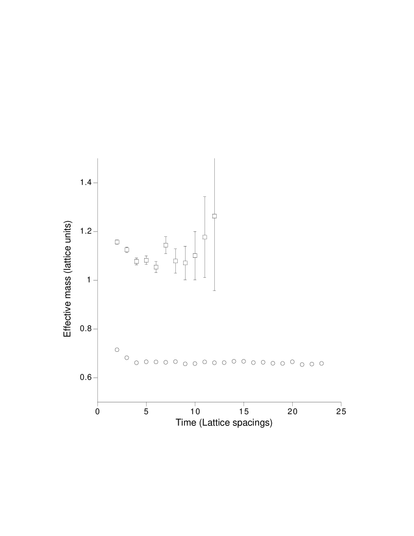
Figure 1: The effective mass, $-\ln\left(\frac{G(T+1)}{G(T)}\right)$, of the ${}^{1}S_{0}$ (circles) and ${}^{1}P_{1}$ (squares) in the quenched simulation.

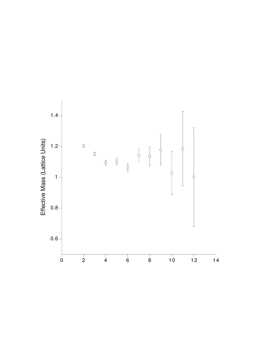
Figure 2: The effective mass, $-\ln\left(\frac{G(T+1)}{G(T)}\right)$, of the ${}^{3}P_{0}$ in the quenched simulation.

An example of the quality of the correlator data is shown in Figures 1 and 2, plots of the effective masses for the ${}^{1}S_{0}$, ${}^{1}P_{1}$ and ${}^{3}P_{0}$ from the simulation using the Landau tadpole factor. The meson propagators were fit with single exponentials over a range of time intervals $(t_{min}:t_{max})$. An indication of the convergence of these fits is given in Table 2, where the fit results are shown for the ${\cal O}(v^{6})$ simulations using the plaquette tadpole factor. The results presented in this table are representative of all of the charmonium spectra we present here. The two $S$-states had a much cleaner signal than the four $P$-states, evident in the lower value for $t_{max}$ used for the $P$-state fits.

Table 3 contains the final results for the quenched charmonium mass fits. We considered the ground-state for each meson propagator to have properly emerged when three consecutive $t_{min}:t_{max}$ intervals gave results that agreed within statistical errors; the meson mass was then taken as the middle of these three values. The masses are given in both lattice units and physical units, using the values for $a^{-1}$ in Table 1 to provide the physical energy scale. The simulated spectra are displayed in Figures 3 and 4, shown against the experimental data.

3.2 Unquenched Results

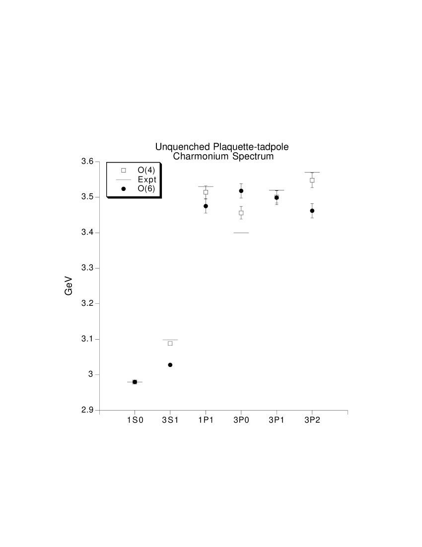
Figure 5: Unquenched charmonium spectrum using $u_{0}^{P}$. Squares represent results obtained to ${\cal O}(v^{4})$, circles represent ${\cal O}(v^{6})$ data. Horizontal lines indicate experimental values.

Given the similar lattice spacings of the MILC configurations and our own quenched ensembles, we have used almost the same parameter set for the unquenched charmonium simulations—the lower half of Table 1 shows the specific parameters used. The results of the unquenched simulations are contained in Table 4, with the physical energy scale set by $a^{-1}=1.21(2)$ GeV, again from the spin-averaged $P$–$S$ splitting. The spectra are shown in Figures 5 and 6.

4 Discussion of the Spectra

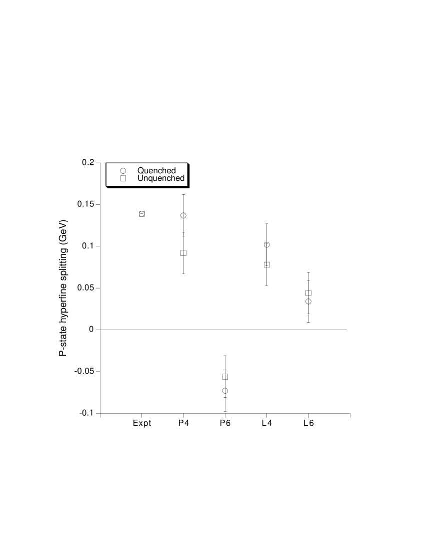
Figure 8: Charmonium $P$-state hyperfine splitting. ‘P4’, ‘P6’ refer to the ${\cal O}(v^{4})$, ${\cal O}(v^{6})$ results obtained with the plaquette tadpole factor; ‘L4’ and ‘L6’ are the Landau tadpole results.

A cursory comparison of the quenched and unquenched results shows that, while the qualitative structure of the spectrum appears, precision NRQCD simulations of the charmonium system have a number of issues yet to be resolved. This is most readily seen in the hyperfine splittings, which are collected in Figures 7 and 8, and compared in Table 5.

Consider first the quenched results. The ${\cal O}(v^{6})$ corrections lead to a disturbingly large decrease in the hyperfine splittings, taking them further away from the experimental values by as much as $60\%$. The situation for the plaquette-tadpole simulations is strikingly bad, where the ${}^{3}P$ states appear in the wrong order. This reversal is corrected in the Landau-tadpole simulations, though the hyperfine splittings are still badly underestimated.

These difficulties are not new—Trottier [4] first drew attention to the large ${\cal O}(v^{6})$ corrections to the $S$-state hyperfine splitting in 1996, and noted a possible problem with the ${}^{3}P$-state ordering. Trottier and Shakespeare [12] examined the effects of the different tadpole definitions $u_{0}^{P}$ and $u_{0}^{L}$ on the $S$-state hyperfine splitting. They performed ${\cal O}(v^{6})$-improved NRQCD simulations using both tadpole schemes, across a wide range of lattice spacings, and drew a number of important conclusions; most notably, the ${\cal O}(v^{6})$ hyperfine corrections with Landau tadpoles were significantly smaller than the plaquette tadpole results.

We have confirmed a number of these results here, and in particular clearly resolved the extremely poor ${}^{3}P$-state behaviour, most notably when $u_{0}^{P}$ is used. This may simply be a problem due to the bare charm mass falling below one in these simulations. However, the $u_{0}^{L}$ simulations lead to a higher bare $c$-quark mass for a given lattice spacing, and the very low $P$-state hyperfine splitting even with $aM_{0}>1$ suggests that these problems extend beyond the size of the bare mass.

4.1 Evidence for Quenching Effects?

The large discrepancies in spin-dependent splittings would be less worrisome if quenching were seen to have a considerable effect on the spectrum, as suggested in [8]. Sadly, this does not seem to be the case. There is some evidence for a difference between the quenched and unquenched simulations in the ${\cal O}(v^{6})$ $S$-hyperfine data, perhaps as much as ten percent. However, given the apparent size of other systematic uncertainties, no great significance can be attached to these differences.

We must address the difference between the quenched and unquenched gluon actions—the MILC configurations were created with the Wilson plaquette action, while we have employed the rectangle-improved action for the quenched lattices. We therefore anticipate an ${\cal O}(a)$ error entangled with the effects of the dynamical quarks. Our quenched ${\cal O}(v^{4})$ results can be compared with the results from Reference [3], where the plaquette action was used at roughly the same lattice spacing. We see a $\sim 10$ MeV difference between the $S$-hyperfine splittings in the two simulations.

We wish to reiterate our goal, however, to see whether the dynamical quark effects are large or small. The $S$-hyperfine splitting, even in relativistic simulations, falls short of experiment by 40 to 50 MeV. An unquenching effect of this magnitude would be visible, even taking differences in gluon action into account. No such effect was observed in these simulations, and we therefore suggest that quenching effects are small in this sense.

This conclusion is supported by results in high-precision $\Upsilon$ simulations [7, 6], where the $P$-state hyperfine splitting is still somewhat underestimated in unquenched simulations of this highly-nonrelativistic system, despite the use of the ${\cal O}(v^{6})$ improved NRQCD action. Very recently, a $10\%$ sea-quark effect was seen in the hyperfine splittings of the charmonium and bottomonium system in Reference [7], but differences between the $n_{f}=0$ and $n_{f}=2$ $P$-state splittings were not significant compared with other systematic uncertainties. Recent results with unquenched lattices in the $B$ meson spectrum have also shown no significant differences between $n_{f}=0$ and $n_{f}=2$ dynamical quark flavours [17].

4.2 Other Systematic Errors

The preceding results suggest that agreement between lattice simulations and experiment in quarkonium systems will likely not improve through the effects of dynamical quarks alone. In the remainder of this section we explore various other systematic errors that impact on heavy-quark simulations, as a contrast to the small quenching effects found above.

4.2.1 The Choice of the Tadpole Factor

We have seen, as others have previously, large differences between results using the Landau tadpole factor $u_{0}^{L}$, and those with the plaquette definition $u_{0}^{P}$. In our own simulations, the size of the ${\cal O}(v^{6})$ corrections with $u_{0}^{L}$ are significantly smaller than the plaquette tadpole results. This is not surprising: the E and B fields are each multiplied by a factor of $u_{0}^{-4}$ in the tadpole-improved theory. On our lattices,

$$\left(\frac{u_{0}^{P}}{u_{0}^{L}}\right)^{4}=\left\{\begin{array}[]{l}1.24\,\,\,\mbox{(Quenched)}\\ 1.30\,\,\,\mbox{(MILC)}\end{array}\right.$$ (19)

Terms in the NRQCD Hamiltonian linear in E or B will differ by as much as $30\%$ between the different tadpole improvement schemes.

As noted earlier, the evidence in favour of Landau tadpoles is strong. Our simulations offer further support, particularly in the ${}^{3}P$-state behaviour, though the more salient issue here is that tadpole effects are at least as important as quenching effects in our simulations.

4.2.2 Radiative Corrections

We expect some effect on the spectrum from high-momentum modes that are cut off by the finite lattice spacing. These high-energy effects may be calculated in perturbative QCD as ${\cal O}(\alpha_{s})$ radiative corrections to the coefficients of the NRQCD expansion, and there are indications that these may be large for the charm quark. Lattice perturbation theory calculations of corrections to $c_{1}$ and $c_{5}$, the ‘kinetic’ terms in Equation (1), have been completed by Morningstar [18]. The corrections are roughly $10\%$ or less for the bottom quark, but rise dramatically as the bare quark mass falls below one (in lattice units). In typical simulations, the bare charm quark mass sits close to unity, and so these corrections may become quite significant.

It is possible to find these radiative corrections without performing long calculations in lattice perturbation theory, by using Monte Carlo simulations at very high values of $\beta$ [19]. Such ‘non-perturbative’ perturbative results have been obtained by Trottier and Lepage [20] for the spin-dependent $c_{4}$ term in the ${\cal O}(v^{4})$ NRQCD Hamiltonian, Equation (1). Unfortunately, radiative corrections to the remaining terms in the NRQCD Hamiltonian have not been calculated to date.

We performed a ‘toy’ simulation to roughly estimate the effects of ${\cal O}(\alpha_{s})$ corrections to all terms in the NRQCD Hamiltonian, replacing the tree level coefficients $c_{i}=1$ with $c_{i}=1\pm\alpha_{s}$. A rough estimate of $\alpha_{s}$ can be made from the (tadpole-improved) parameters of our simulations,

$$\alpha_{s}(\pi/a)\simeq\alpha_{lat}^{TI}+{\cal O}(\alpha^{2})\simeq\frac{g^{2}}{4\pi}=\frac{6}{4\pi\beta u_{0}^{4}}\,.$$ (20)

For our values of $\beta$ and $u_{0}$, this gives $\alpha_{s}\sim 0.15$–$0.2$. For the three terms in the Hamiltonian where perturbative analysis has been performed, we used the calculated values [18, 20]; for the remaining terms, we varied the coefficients between 0.8 and 1.2.

Altering the coefficients in this way, we found that the charmonium $S$- and $P$-hyperfine splittings changed by as much as $10$–$40\%$, depending on the sign of the corrections for each individual $c_{i}$. While this is only a crude estimate, it is clear that the effects of radiative corrections may be as important as quenching effects for heavy-quark systems. Accurate determinations of the remaining ${\cal O}(\alpha_{s})$ corrections are sorely needed.

4.2.3 Improving the Evolution Equation

The evolution equation we presented in Section 2 for the heavy-quark propagator, Equation (10), contains better-than-linear approximations to the exponential $e^{Ht}$ for the terms involving the zeroth-order Hamiltonian $H_{0}$, but only a linear approximation for the correction terms $\delta H$. Noting that the high-order corrections are quite large for charmonium, it is conceivable that this lowest-order approximation is too severe. A similar conclusion was made by Lewis and Woloshyn of their NRQCD simulations of the $D$ meson spectrum [21]. The authors were able to remove some spurious effects due to large vacuum expectation values of one of the high-order terms in their NRQCD Hamiltonian [22], by improving the exponential approximation for the $\delta H$ terms in the evolution equation.

The coefficients of the ${\cal O}(v^{6})$ terms include high powers of $M_{0}^{-1}$ and $u_{0}^{-1}$, and it is conceivable that for the charm quark, with $aM_{0}\sim 1$, the $(1-a\delta H_{v^{6}})$ approximation is poor. We examined this possibility for the ${\cal O}(v^{6})$ terms, by using an improved form for the evolution equation that incorporates a ‘stabilisation’ parameter for the correction terms, with the replacement

$$(1-a\delta H)\to\left(1-\frac{a\delta H}{s_{\delta}}\right)^{s_{\delta}}\,.$$ (21)

We have performed a simulation with this alteration to the evolution equation, with $s_{\delta}=4$. Otherwise, all other parameters were kept the same as the previous Landau-tadpole quenched simulations. In general, altering the evolution equation will lead to a change in the bare charm quark mass $M_{0}$. In this case we found that $M_{0}=1.15$ once again gave a value of $3.0(1)$ GeV for the ${}^{1}S_{0}$ mass.

The the improved evolution equation altered the $S$-hyperfine splitting significantly, increasing it by roughly $40\%$ to $70$ MeV. The statistical uncertainties in the $P$-hyperfine splittings were large, though a similar increase seems likely. These results suggest the linear approximation $(1-a\delta H)$ typically used in NRQCD simulations is not sufficiently accurate for the large corrections encountered at the charm quark mass.

5 Conclusions

Lattice NRQCD simulations of heavy-quark systems have evolved greatly over the last decade. By incorporating high-order interaction terms to counter relativistic and discretisation errors, simulations now routinely produce results that agree with experiment at the $10$–$30\%$ level. However, stubborn discrepancies remain in highly-improved simulations, typically performed in the quenched approximation, or at tree-level in the ${\cal O}(\alpha_{s})$ expansion, or both. To proceed further, all remaining systematic errors must be addressed.

Past studies strongly suggest that the NRQCD expansion converges slowly for the charm quark, with the leading and next-to-leading order corrections apparently oscillating in sign. To ${\cal O}(v^{6})$, the hyperfine spin-splittings fall short of experimental values by $50\%$ or more. Without knowing the magnitude of the next-order corrections in the velocity expansion, the question of reducing the disparities in the charmonium spectrum seems academic.

While the NRQCD approach appears to be problematic for the charmonium system, relativistic lattice formalisms have their share of difficulties. Simulations of charmonium with a variety of quark actions—NRQCD, the Fermilab actions, the D234 action—all underestimate the $S$-hyperfine splitting by at least $40$ MeV (see [4] for a good summary).

There are sound reasons for estimating the size of dynamical quark effects in the charmonium system. Some have suggested the remaining hyperfine discrepancy is due to quenching; estimates of the effects of dynamical quark loops range as high as $40\%$ [8]. Our results indicate this is unlikely to be the case—we find at most a $10\%$ difference between our quenched and unquenched hyperfine splittings. As the quenching effects are apparently small for the range of different quark interactions present in the NRQCD action, we suggest that they will also be small across other quark actions.

We recognise several shortcomings in our study: we have used different gluon actions for quenched and unquenched simulations, we have only examined the effects of unquenching at a single dynamical quark mass and a single lattice spacing, and we have not attempted to extrapolate to the physical case of three light sea quark flavours. The first of these issues was discussed in Section 4.1 above. To address the other objections with further simulations is beyond our present computational resources. In any case, such efforts are perhaps justified in simulations of the $b$ quark, where systematic uncertainties are under better control and quenching effects are probably of comparable size to discretisation and radiative effects. For the charm system however, the much larger high-order relativistic errors and the large tadpole corrections dominate the effects of quenching.

The sensitivity of the NRQCD corrections to the choice of tadpole factor is well established. This sensitivity should disappear with a higher-order treatment of the tadpole loops (and other radiative corrections) in lattice simulations. In practice, such a treatment is not yet available, and some choice for the tadpole factor is required. Our results add to the growing list of evidence if favour of calculating the tadpole correction factor from the mean link in the Landau gauge, in preference to the plaquette definition.

The large effects we have encountered due to instabilities in the evolution equation should also be investigated further. These instabilities are doubtless amplified in simulations of the charm quark, where the convergence of the NRQCD expansion is already questionable. Using an improved evolution equation, as we have demonstrated, may bring the NRQCD approach into agreement with other quenched relativistic results for charmonium.

Further, we have shown that ${\cal O}(\alpha_{s})$ radiative corrections may shift the spin-splittings by as much as $40\%$. While this is a crude estimate, the possibility of such sizeable corrections in comparison with the small quenching effect gives us pause for consideration. Of particular note are unquenched results for the $\Upsilon$ spectrum in [6], using the ${\cal O}(v^{6})$ Hamiltonian, which indicate that remaining discrepancies with experiment are at the ten percent level—conceivably within the reach of radiative corrections. Perturbative calculations of the remaining radiative corrections to the NRQCD coefficients, and those in other actions as well, will likely be necessary in the near future.

We thank Howard Trottier and Randy Lewis for stimulating discussions. This work has been supported by the Natural Sciences and Engineering Research Council of Canada.

$\beta$	$u_{0}^{P}$	$u_{0}^{L}$	$a$ (fm)	$a^{-1}$ (GeV)	$aM_{0}$	$M_{k}$	$s$
Quenched
2.52	0.874		0.168(3)	1.17(2)	0.81	3.0(1)	6
2.10		0.829	0.181(3)	1.09(2)	1.15	3.0(1)	4
Unquenched
5.415	0.854		0.163(3)	1.21(2)	0.82	2.9(1)	6
5.415		0.800	0.163(3)	1.21(2)	1.15	2.9(1)	4

Table 1: Parameters used in charmonium simulations. The lattice volume is $12^{3}\times 24$ for the quenched simulations, and $16^{3}\times 32$ for the unquenched simulations. $M_{k}$ is the kinetic mass of the ${}^{1}S_{0}$ state; $s$ is the NRQCD stability parameter in Equation (1).

$t_{min}:t_{max}$	${}^{1}S_{0}$	${}^{3}S_{1}$	${}^{3}S_{1}$ - ${}^{1}S_{0}$
2:24	0.6646(4)	0.7000(5)	—
3:24	0.6630(5)	0.6984(5)	0.03659(9)
4:24	0.6625(5)	0.6979(6)	0.03661(11)
5:24	0.6624(6)	0.6977(7)	0.03645(13)
6:24	0.6623(7)	0.6976(7)	0.0364(2)
7:24	0.6623(7)	0.6976(8)	0.0364(2)

$t_{min}:t_{max}$	${}^{1}P_{1}$	${}^{3}P_{0}$	${}^{3}P_{1}$	${}^{3}P_{2}$
2:14	1.109(4)	1.159(4)	1.138(5)	1.082(4)
3:14	1.093(5)	1.127(7)	1.113(6)	1.072(5)
4:14	1.085(7)	1.122(10)	1.102(9)	1.065(6)
5:14	1.087(10)	1.139(15)	1.107(12)	1.067(9)
6:14	1.091(13)	1.14(2)	1.114(18)	1.067(12)

Table 2: Examples of fits to quenched charmonium propagators. The fit results are shown for the plaquette-tadpole simulation, for various sets of $(t_{min}:t_{max})$. Single exponential fits are used for individual masses, and a ratio fit is used to extract the $S$-state hyperfine splitting. Italicised entries indicate the final results.

State	$u_{0}^{P}$		$u_{0}^{L}$
	${\cal O}(v^{4})$	${\cal O}(v^{6})$	${\cal O}(v^{4})$	${\cal O}(v^{6})$
${}^{1}S_{0}$	0.5733(5)	0.6625(5)	0.1708(4)	0.2297(4)
${}^{3}S_{1}$	0.6635(8)	0.6979(6)	0.2466(6)	0.2802(5)
${}^{1}P_{1}$	1.034(8)	1.085(7)	0.643(7)	0.696(7)
${}^{3}P_{0}$	0.966(7)	1.122(10)	0.576(6)	0.661(7)
${}^{3}P_{1}$	1.006(8)	1.102(9)	0.628(7)	0.695(8)
${}^{3}P_{2}$	1.088(8)	1.065(6)	0.669(9)	0.692(7)
${}^{3}S_{1}-$${}^{1}S_{0}$	0.0910(3)	0.0365(1)	0.0778(3)	0.0521(2)

State	$u_{0}^{P}$		$u_{0}^{L}$		Expt
	${\cal O}(v^{4})$	${\cal O}(v^{6})$	${\cal O}(v^{4})$	${\cal O}(v^{6})$
${}^{3}S_{1}$	3.086(2)	3.022(2)	3.066(2)	3.036(1)	3.097
${}^{1}P_{1}$	3.517(17)	3.470(17)	3.499(18)	3.479(17)	3.526
${}^{3}P_{0}$	3.439(16)	3.522(20)	3.426(15)	3.441(17)	3.417
${}^{3}P_{1}$	3.486(17)	3.488(17)	3.483(18)	3.478(18)	3.511
${}^{3}P_{2}$	3.576(17)	3.449(16)	3.528(22)	3.475(17)	3.556
${}^{3}S_{1}-$${}^{1}S_{0}$	0.106(3)	0.042(2)	0.086(2)	0.056(2)	0.118

Table 3: Quenched charmonium masses in lattice units (top) and GeV (bottom). The scale is set by $a^{-1}$ in Table 1.

State	$u_{0}^{P}$		$u_{0}^{L}$
	${\cal O}(v^{4})$	${\cal O}(v^{6})$	${\cal O}(v^{4})$	${\cal O}(v^{6})$
${}^{1}S_{0}$	0.5501(3)	0.6279(3)	0.0581(3)	0.1155(3)
${}^{3}S_{1}$	0.6363(5)	0.6668(4)	0.1278(4)	0.1658(4)
${}^{1}P_{1}$	0.988(7)	1.030(10)	0.485(7)	0.537(6)
${}^{3}P_{0}$	0.937(6)	1.020(8)	0.433(6)	0.503(6)
${}^{3}P_{1}$	0.977(7)	1.050(10)	0.476(7)	0.531(7)
${}^{3}P_{2}$	1.016(9)	1.065(5)	0.497(9)	0.540(7)
${}^{3}S_{1}-$${}^{1}S_{0}$	0.0884(3)	0.0365(2)	0.0719(2)	0.0522(1)

State	$u_{0}^{P}$		$u_{0}^{L}$		Expt
	${\cal O}(v^{4})$	${\cal O}(v^{6})$	${\cal O}(v^{4})$	${\cal O}(v^{6})$
${}^{3}S_{1}$	3.087(2)	3.028(2)	3.068(2)	3.043(1)	3.097
${}^{1}P_{1}$	3.514(17)	3.475(17)	3.500(17)	3.486(16)	3.526
${}^{3}P_{0}$	3.456(15)	3.518(20)	3.437(15)	3.445(15)	3.417
${}^{3}P_{1}$	3.501(17)	3.499(17)	3.490(17)	3.479(17)	3.511
${}^{3}P_{2}$	3.548(21)	3.462(16)	3.515(21)	3.489(17)	3.556
${}^{3}S_{1}-$${}^{1}S_{0}$	0.107(2)	0.049(1)	0.087(2)	0.062(1)	0.118

Table 4: Unquenched charmonium masses in lattice units (top) and GeV (bottom). The scale is set by $a^{-1}$ in Table 1.

			$S$-state hyperfine	$P$-state hyperfine
			${}^{3}S_{1}-$${}^{1}S_{0}$	${}^{3}P_{2}-$${}^{3}P_{0}$
Experiment			0.118	0.139
${\cal O}(v^{4})$	Quenched	$u_{0}^{P}$	0.106(2)	0.14(2)
		$u_{0}^{L}$	0.086(2)	0.10(2)
	Unquenched	$u_{0}^{P}$	0.108(2)	0.10(2)
		$u_{0}^{L}$	0.087(2)	0.08(2)
${\cal O}(v^{6})$	Quenched	$u_{0}^{P}$	0.042(1)	-0.07(2)
		$u_{0}^{L}$	0.056(1)	0.033(15)
	Unquenched	$u_{0}^{P}$	0.049(1)	-0.023(17)
		$u_{0}^{L}$	0.062(1)	0.044(15)

Table 5: Quenched and unquenched $S$-state and $P$-state hyperfine splittings for both $u_{0}^{P}$ and $u_{0}^{L}$ simulations.

Figure 3: Quenched charmonium spectrum using $u_{0}^{P}$. Squares represent results obtained to ${\cal O}(v^{4})$, circles represent ${\cal O}(v^{6})$ data. Horizontal lines indicate experimental values.

Figure 4: Quenched charmonium spectrum using $u_{0}^{L}$. Squares represent results obtained to ${\cal O}(v^{4})$, circles represent ${\cal O}(v^{6})$ data. Horizontal lines indicate experimental values.

Figure 6: Unquenched charmonium spectrum using $u_{0}^{L}$. Squares represent results obtained to ${\cal O}(v^{4})$, circles represent ${\cal O}(v^{6})$ data. Horizontal lines indicate experimental values.

Figure 7: Charmonium $S$-state hyperfine splitting. ‘P4’, ‘P6’ refer to the ${\cal O}(v^{4})$, ${\cal O}(v^{6})$ results obtained with the plaquette tadpole factor; ‘L4’ and ‘L6’ are the Landau tadpole results.

References

- [1] B.A. Thacker and G.P. Lepage, Phys. Rev. D 43 (1991) 196.
- [2] G.P. Lepage, L. Magnea, C. Nakhleh, U Magnea and K. Hornbostel, Phys. Rev. D 46 (1992) 4052.
- [3] C. T. H. Davies et al., Phys. Rev. D 52 (1995) 6519; hep-lat/9506026.
- [4] H. D. Trottier, Phys. Rev. D 55 (1997) 6844; hep-lat/9611026.
- [5] T. Manke et al., Phys. Lett. B 408 (1997) 308; hep-lat/9706003.
- [6] N. Eicher et al., Phys. Rev. D 57 (1998) 4080; hep-lat/9709002.
- [7] CP-PACS collaboration, T. Manke et al., hep-lat/0005022.
- [8] A. X. El-Khadra, Nucl. Phys. B (Proc. Suppl.) 30 (1993) 449; hep-lat/9211046.
- [9] P. Boyle, submitted for publication, see hep-lat/9903017.
- [10] See, for example, the talk presented by Y. Kuramashi at the Division of Particles and Fields Conference 99, UCLA, USA 1999, and hep-lat/9904003; also see R. D. Kenway, Nucl. Phys. B (Proc. Suppl.) 73 (1999) 16, hep-lat/9810054.
- [11] G. P. Lepage, in procedings of Perturbative and Nonperturbative Aspects of Quantum Field Theory, 35th Internationale Universitätwochen für Kern- und Teilchenphysik, Schladming, Austria (March 2–9, 1996), H. Latal and W. Schweiger (editors), Springer (1996); hep-lat/9607076.
- [12] Norman Shakespeare and Howard Trottier, Phys. Rev. D 58 (1998) 034502; hep-lat/9802038.
- [13] N. H. Shakespeare and H. D. Trottier, Phys. Rev. D 59 (1999) 014502, and hep-lat/9803024.
- [14] M. Luscher et al., Nucl. Phys. B 491 (1997) 323; see also G. P. Lepage, invited talk at the Workshop on Lattice QCD on Parallel Computers (Tsukuba, March 1997), hep-lat/9707026.
- [15] C. R. Allton et al., Phys. Rev. D 47 (1993) 5128.
- [16] The unquenched configurations were made available by the MILC collaboration, through the Gauge Connection, http://qcd.nersc.gov/
- [17] S. Collins et al., Phys. Rev. D 60(1999) 074504; hep-lat/9901001.
- [18] Colin J. Morningstar, Phys. Rev. D 50 (1994) 5902; hep-lat/9406002.
- [19] W. Dimm, G. P. Lepage, and P. B. Mackenzie, Nucl. Phys. B (Proc. Suppl.) 42 (1995) 403.
- [20] H. D. Trottier and G. P. Lepage, submitted for publication, see hep-lat/9910018; H. D. Trottier and G. P. Lepage, Nucl. Phys. B (Proc. Suppl.) 63 (1998) 865, and hep-lat/9710015.
- [21] R. Lewis and R. M. Woloshyn, submitted for publication, see hep-lat/9803004.
- [22] The term considered in [21] appears at in the NRQCD expansion, so we have not included it in our simulations.