Sea Quark Effects on Quarkonia

Abstract

We study the effects of two dynamical sea quarks on the spectrum of heavy quarkonia. Within the non-relativistic approach to Lattice QCD we found sizeable changes to the hyperfine splitting, but we could not observe any changes for the fine structure. We also investigated the scaling behaviour of our results for several different lattice spacings.

I Introduction

The experimental efforts to pin down the parameters of the Standard Model have been paralleled by intense theoretical attempts to provide experimentalists with non-perturbative constraints from Quantum Chromodynamics (QCD). It is hoped that Lattice QCD will ultimately provide such important information. To this end it is crucial to understand and control the systematic errors in numerical calculations, which rely on extrapolations and interpolations to the physical point. This important task is particularly demanding for heavy quark phenomenology, where one has to describe accurately both the light and heavy quarks in the system.

In particular the inclusion of light dynamical fermions in the gluon background is still a daunting task and requires the largest fraction of computational resources. In the past these restrictions led to the so-called quenched approximation, in which only valence quarks are allowed to propagate in a purely gluonic background, whereas the virtual creation of sea quarks is ignored. We have shown in a recent work [1] that this results in systematic deviations in the lattice prediction of the light hadron spectrum from the observed experimental data. More recently it has also been found that the inclusion of two dynamical sea quarks has a significant effect on the light hadron spectrum and quark masses [2, 3]. This is of course analogous to QED, where the inclusion of all higher order effects, which could be made through perturbation theory, resulted in an impressive agreement with experimental observations. A distinctive aspect of QCD is that a proper non-perturbative treatment is in order so as to provide high-precision tests of this theory. Here we take this as our motivation to study heavy quarkonia in the presence (and absence) of dynamical sea quarks.

Heavy quark systems have long been considered an ideal testing ground for QCD and they have triggered the development of static potential models [4] and heavy quark effective field theories [5]. On the lattice, heavy quarks have frequently been studied using a non-relativistic approach to QCD (NRQCD [6]) or a relativistic formulation promoted by the Fermilab group [7]. Both provide effective descriptions to deal with large scale differences, which are difficult to accommodate on conventional lattices. NRQCD has been quite successful in reproducing the spin-independent spectrum of heavy quarkonia [8] owing to the fact that the quarks within such mesons move with small velocities $v$ such that $v^{2}\ll c^{2}$.

As an effective field theory the predictive power of NRQCD relies on the control of higher dimensional operators, which have to be matched to the non-relativistic expansion of QCD. This has been the subject of many previous studies [9, 10, 11]. As a result of these works it seemed plausible that bottomonium states could be accurately described in the NRQCD approach, whereas the spin structure of charmonium is very sensitive to the higher order relativistic corrections [12, 13].

Within the NRQCD framework sea quark effects on the heavy quarkonium spectra have previously been studied at a lattice spacing of $a\approx 0.1$ fm using the Kogut-Susskind [14] or the Wilson [15] action for sea quarks. Here we present results for three lattice spacings in the range $a\approx 0.2-0.1$ fm, paying particular attention to the dependence on the sea quark mass and scaling properties. Our gauge configurations are generated with a renormalization-group (RG)-improved gluon action [16] and a tadpole-improved clover quark action [17] for two dynamical flavours [2]. Some measurements are also made on quenched configurations generated with the same gluon action for making direct comparisons of dynamical and quenched results.

In Section II we introduce the actions which we use in our calculation. In Section III we give the details of our simulation, meson operators and fitting methods. Our results are discussed in Section IV and Section V concludes this paper.

II Actions

A Glue: RG-Improved Action

Since there is no unique discretisation of the continuum gluon action one can employ a set of operators to cancel some of the discretisation errors in the lattice action. The most common choice is to simply add a rectangular $1\times 2$ plaquette, ${\rm Tr}R_{\mu\nu}$, to the standard Wilson action, ${\rm Tr}P_{\mu\nu}$,

$$S_{\rm g}(g^{2})=\frac{1}{g^{2}}\left\{c_{0}{\rm Tr}P_{\mu\nu}+c_{1}{\rm Tr}R_{\mu\nu}\right\}~{}~{},$$ (1)

where ${\rm Tr}$ denotes the trace over all indices and $c_{0}+8c_{1}=1$. All such choices have the same continuum limit, but different discretisation errors. Here we adopt a prescription which is motivated by an RG-analysis of the pure gauge theory ($c_{1}=-0.331$ [16]). This has proven to be a suitable choice compared to, say, the Symanzik-improved action ($c_{1}=-1/12$), for reducing scaling violation on coarse lattices. Instead of the coupling constant squared, $g^{2}$, we often quote the value of $\beta\equiv 6/g^{2}$.

B Light Quarks: Clover Action

The standard discretisation of the fermion action removes the doublers at the expense of ${\cal O}(a)$ discretisation errors. It is possible to remove these errors by adding a single operator (the clover term) as first suggested in [17]:

$$S_{\rm q}(g^{2},m_{q})=\bar{q}~{}Q~{}q=\bar{q}~{}(/\hskip-7.0pt\Delta+m_{q})~{}q+ar~{}\bar{q}~{}\Delta^{2}~{}q-c_{sw}(g^{2})~{}ar~{}\frac{ig}{4}\bar{q}~{}\sigma_{\mu\nu}F_{\mu\nu}~{}q~{}~{}.$$ (2)

Here the second term removes the doublers a la Wilson and the last is to reduce the resulting ${\cal O}(a)$ errors. We choose $r=1$ and $c_{sw}=(1-0.1402~{}g^{2})^{-3/4}$. For the latter we follow the tadpole prescription of [18], which has been shown to improve the convergence of lattice perturbation theory significantly. Our choice is based upon the perturbative plaquette values as determined in [16]. To one-loop order our choice differs from the correct value [19] only by $0.008g^{2}$. Hence we expect only small ${\cal O}(\alpha a)$ scaling violations due to radiative corrections from the clover action, and ${\cal O}(a^{2})$ errors from the gluon action.

In our simulations we work with two flavours of degenerate quarks of a common mass: $m_{q}=m_{u}=m_{d}$. For further reference, it is customary to replace the bare quark mass by the hopping parameter: $\kappa\equiv 1/2(m_{q}a+4)$. Since the direct simulation of realistic light Wilson quarks is not feasible on present-day computers we study the spectrum at a sequence of different $\kappa$.

C Heavy Quarks: NRQCD

With the above actions we generated full QCD dynamical configurations on lattices of about 2.5 fm in spatial extent and lattice spacings ranging from approximately 0.1 to 0.2 fm. Such lattices are particularly suited to study light quark physics which is determined by a single scale: $\Lambda_{QCD}\approx 200$ MeV. However, for systems containing slow-moving and heavy quarks we have to adjust the theoretical description to take into account all the non-relativistic scales: mass ($m_{Q}$), momentum ($m_{Q}v$) and kinetic energy ($m_{Q}v^{2}$). In this work we implement the NRQCD formulation to propagate the heavy quarks in a given gluon background. This approach has met with considerable success for b-quarks [9, 11]. Also charm quarks have previously been studied in this framework [12, 13].

Whereas the relativistic boundary value problem requires several iterations to determine the quark propagator, the NRQCD approach has the numerical advantage to solve the two-spinor theory as a much simpler initial value problem. The forward propagation of the source vector, $S({\bf x})$, is described by:

$$G({\bf x},t+1) = \left(1-\frac{a}{2}\delta H\right)\left(1-\frac{aH_{0}}{2n}\right)^{n}U_{t}^{{\dagger}}(x)\left(1-\frac{aH_{0}}{2n}\right)^{n}\left(1-\frac{a}{2}\delta H\right)G({\bf x},t)~{}~{},~{}~{}~{}t\geq 1~{}~{},$$ (3)

$$G({\bf x},1) = \left(1-\frac{a}{2}\delta H\right)\left(1-\frac{aH_{0}}{2n}\right)^{n}U_{t}^{{\dagger}}(x)\left(1-\frac{aH_{0}}{2n}\right)^{n}\left(1-\frac{a}{2}\delta H\right)S({\bf x})~{}~{},~{}~{}~{}t=0~{}~{},$$ (4)

where

$$H_{0} = -\frac{\Delta^{2}}{2m_{Q}}~{}~{},$$ (5)

$$\delta H = -c_{0}\frac{\Delta^{4}}{8m_{Q}^{3}}-c_{1}\frac{1}{2m_{Q}}\sigma\cdot g{\bf\tilde{B}}+c_{2}\frac{i}{8m_{Q}^{2}}(\tilde{\Delta}\cdot g{\bf\tilde{E}}-g{\bf\tilde{E}}\cdot\tilde{\Delta})-c_{3}\frac{1}{8m_{Q}^{2}}\sigma\cdot(\tilde{\Delta}\times g{\bf\tilde{E}}-g{\bf\tilde{E}}\times\tilde{\Delta})$$ (8)

$$-c_{4}\frac{1}{8m_{Q}^{3}}\{\Delta^{2},\sigma\cdot g{\bf\tilde{B}}\}-c_{5}\frac{1}{64m_{Q}^{3}}\{\Delta^{2},\sigma\cdot(\tilde{\Delta}\times g{\bf\tilde{E}}-g{\bf\tilde{E}}\times\tilde{\Delta})\}-c_{6}\frac{i}{8m_{Q}^{3}}\sigma\cdot g{\bf\tilde{E}}\times g{\bf\tilde{E}}$$

$$-c_{7}\frac{a\Delta^{4}}{16nm_{Q}^{2}}+c_{8}\frac{a^{2}\Delta^{(4)}}{24m_{Q}}~{}~{}.$$

The improved lattice operators $\tilde{\Delta}_{i},\tilde{\bf E}$ and $\tilde{\bf B}$ are defined as in [9]. Other discretisations of NRQCD have been suggested in the past but they differ only at higher order in the lattice spacing. Here we follow [11, 15] and employ a formulation which includes all spin terms up to $O(mv^{6})$ in non-relativistic expansion of QCD. On the coarsest lattice we checked explicitly that our equation (4) gives the same hyperfine splitting as from the asymmetric version employed in [11]. The parameter $n$ was introduced to stabilise the evolution equation against high momentum modes. This is standard in such diffusive problems, but one should keep in mind that a change in $n$ will have to be accompanied by a change in $m_{Q}$ to simulate the same physical system. Alternatively one could decrease the temporal lattice spacing to prevent the high momentum modes from blowing up [20].

For a single quark source at point ${\bf y}$ we have $S({\bf x})=\delta^{(3)}({\bf x,y})$, but we also propagate extended objects with the same evolution equation (4). The operator $H_{0}$ is the leading kinetic term and $\delta H$ contains the relativistic corrections. The last two terms in $\delta H$ are present to correct for lattice spacing errors in temporal and spatial derivatives. For the derivatives we use the improved operators defined in [9] and we also replace the standard discretized gauge field $F_{\mu\nu}$ by

$$\tilde{F}_{\mu\nu}=\frac{5}{3}F_{\mu\nu}-\frac{1}{6}\left(U_{\mu}(x)F_{\mu\nu}(x+\mu)U_{\mu}^{{\dagger}}(x)+U_{-\mu}(x)F_{\mu\nu}(x-\mu)U_{-\mu}^{{\dagger}}(x)-(\mu\leftrightarrow\nu)\right)~{}~{}.$$ (9)

With this prescription we aimed to achieve an accuracy of ${\cal O}(a^{4})$ for the heavy quark sector. Of course we also expect terms of ${\cal O}(\alpha a^{2})$ due to radiative corrections to this leading order result. In principle, we have to determine all coefficients in (8) by (perturbative or non-perturbative) matching to relativistic continuum QCD. Just as for the light quark sector we rely on a mean-field treatment of all gauge links to account for the leading radiative corrections. However, there is no unique prescription for such an improvement and several different schemes have been employed in the past. More recently it has been suggested that the average link variable in the Landau gauge should be less sensitive to radiative corrections since the gauge fields in Landau gauge have less UV fluctuations [21]. Here we adopt this view and divide all links by the appropriate tadpole coefficient at each value of $(\beta,\kappa)$:

$$U_{\mu}(x)\to U_{\mu}(x)/u_{0L}~{}~{},~{}~{}u_{0L}\equiv\frac{1}{3}\langle{\rm Tr}U_{\mu}\rangle_{LG}~{}~{}.$$ (10)

An alternative and gauge-invariant implementation of mean-field improvement that has frequently been used in the past forces the average plaquette, $P_{\mu\nu}$, to unity:

$$U_{\mu}(x)\to U_{\mu}(x)/u_{0P}~{}~{},~{}~{}u_{0P}\equiv\frac{1}{3}\langle{\rm Tr}P_{\mu\nu}\rangle^{1/4}~{}~{}.$$ (11)

In some selected cases we have also implemented this method to estimate the effect of unknown radiative corrections to the renormalisation coefficients, $c_{i}$. In all applications of (8) we set them to their tree-level value 1. We denote as ${\cal O}(mv^{6},a^{2})$ the evolution equation which includes all spin-dependent operators up to ${\cal O}(mv^{6})$ and where all operators have been improved to reduce the ${\cal O}(a^{2})$ errors.

III Simulation

A Updates, Trajectories and Autocorrelations

The gauge field configurations with two dynamical sea quarks used for the present study were generated on the CP-PACS supercomputer at the Center for Computational Physics, University of Tsukuba. They can be classified by two parameters, $(\beta,\kappa)$, which determine the lattice spacing and the sea quark mass. A standard hybrid Monte Carlo algorithm is used to incorporate the effects of the fermion determinant. For the matrix inversion we implemented the BiCGStab algorithm. To reduce the autocorrelations between separate measurements we only used every fifth or tenth trajectory and binned the remaining data until the statistical error was independent of the bin size. In Tab. I we list the number of trajectories we generated for each set of couplings along with the other simulation parameters and the actual number of configurations we used in this study; for more details see [2]. The subsequent determination of the quarkonium spectrum is subject of this work.

Since there has been no previous study of heavy quarkonia using the RG action for the gluon sector, we also supplemented our calculation by a comparative quenched calculation. The coupling constant $\beta$ of these quenched configurations were chosen so that the string tension of the static quark-antiquark potential matches that of one of the dynamical runs. The parameters of these runs are also given in Tab. I.

B Meson Operators

To extract meson masses we calculate two-point functions of operators with appropriate quantum numbers. In a non-relativistic setting gauge-invariant meson operators can be constructed from the two-spinors $\chi^{{\dagger}}(x)$, $\Psi(y)$ and a Wilson line, $W(x,y):~{}\chi^{{\dagger}}(x)W(x,y)\Psi(y)$. The construction of meson states with definite $J^{PC}$ from those fundamental operators is standard [22] (on the lattice $J$ labels the irreducible representations of the octahedral group ($J=A_{1},A_{2},T_{1},T_{2},E$)).

Since here we are only interested in S and P-states it is sufficient to consider $\chi^{{\dagger}}(x)\Psi(x)$ and $\chi^{{\dagger}}(x)\Delta_{i}\Psi(x)$, respectively. The corresponding spin-triplets can be constructed by inserting the Pauli matrices into those bilinears. We also sum over different polarisations to increase the statistics.

The overlap of those simplistic operators with the state of interest can be further improved upon. One way is to employ wavefunctions, which try to model the ground state more accurately. This requires assumptions about the underlying potential and gauge-fixed configurations. We decided to use a gauge-invariant smearing technique, which regulates the extent of the lattice operator, with a single parameter $\epsilon$:

$$\chi^{\dagger}(x)~{}\hat{O}~{}\Psi(x)\to\chi^{\dagger}(x)~{}\hat{O}~{}(1-\epsilon\Delta^{2})^{10}~{}\Psi(x)~{}~{}.$$ (12)

For computational ease we limited this procedure to 10 smearing iterations and implemented it only at the source. From such operators we obtain the meson correlators as a Monte Carlo average over all configurations

$${\rm C}_{\epsilon}(x,y)=\langle{\bf tr}\left[G^{{\dagger}}(x,y)~{}\hat{O}~{}G(x,y)~{}(1-\epsilon\Delta^{2})^{10}~{}\hat{O}^{\dagger}~{}\right]\rangle~{}~{},$$ (13)

where ${\bf tr}$ denotes contraction over all internal degrees of freedom.

For the smeared propagator we solve (4) with $S({\bf x,y})=\delta({\bf x,y})~{}(1-\epsilon\Delta^{2})^{10}~{}\hat{O}^{\dagger}$. We fix the origin at some (arbitrary) lattice point $y=({\bf y},0)$. This creates a meson state with all possible momenta. In practice we employed up to 8 spatial sources on every configuration. This is permissible since heavy quarkonia are small compared to the lattice extent of about 2.5 fm. We explicitly checked the independence of such measurements by binning. At the sink, $x=({\bf x},t)$, we perform a Fourier transformation to project the correlator onto a given momentum eigenstate:

$${\rm C}_{\epsilon,t}({\bf p})=\sum_{\bf x}C_{\epsilon}({\bf x},t)\exp{(-i{\bf px})}~{}~{}.$$ (14)

In the trivial case of zero momentum this amounts to simply summing over all spatial ${\bf x}$.

C Fitting

Since there is no backward propagation of the heavy quark in our framework, we can fit the meson propagators to the exponential form:

$$y_{\epsilon,t}(a_{i},E_{i})=\sum_{i=1}^{\rm n_{fit}}~{}a_{i}(\alpha,{\bf p},\epsilon)~{}e^{-E_{i}(\alpha,{\bf p})~{}t}~{}~{}.$$ (15)

This is the theoretical prediction for a multi-exponential decay of a state with momentum ${\bf p}$ and quantum numbers $\alpha$ along Euclidean time $t$. Different choices for the smearing parameter $\epsilon$ will result in different overlaps with the ground state and the higher excited states of the same quantum number. In practice it is difficult to project directly onto a given state, so we chose to extract the ground state from multi-exponential correlated fits. In some cases we were also able to extract the first excited states reliably from our data. The simplest way to visualise our data is by means of effective mass plots, which are expected to display a plateau for long Euclidean times. In Fig. 1 we show a representative plot for one set of simulation parameters.

Correlations between different times, $t$, and different smearing radii, $\epsilon$, of the meson propagator $C_{\epsilon,t}$ are taken into account by employing the full covariance matrix for the $\chi^{2}$-minimisation:

$$\chi^{2}({\bf\pi})\equiv\sum_{r,s=1}(C_{r}-y_{r}({\bf\pi}))~{}\Gamma_{rs}^{-1}~{}(C_{s}-y_{s}({\bf\pi})),~{}~{}~{}~{}~{}\frac{\partial\chi^{2}}{\partial\pi_{k}}\left({\bf\bar{{\bf\pi}}}\right)=0~{}~{}.$$ (16)

Here, in order to ease the notation, we introduced multi-indices ($r=[\epsilon,t]$) for the data points and ${\bf\pi}=[a_{i},E_{i}]$ for the parameters.

Our statistical ensembles are large enough to determine the covariance matrix, $\Gamma_{rs}^{-1}$, with sufficient accuracy. Therefore the inversion of this matrix did not present a problem. For the spin splittings we applied (15) also to the ratio of two propagators, $C(\alpha_{1})/C(\alpha_{2})$. In this way we utilized correlations between states of different quantum numbers to obtain improved estimates for their energy difference.

Statistical fluctuations in the data cause fluctuations in the fit results determined by (16). We estimate the covariance matrix, $\Delta_{kl}$, of the fitted parameters, $\pi_{k}$, from the inverse of $(\partial^{2}\chi^{2})/(\partial\pi_{k}\partial\pi_{l})$. We have checked these errors against bootstrap errors which gave consistent results. We also require consistent results as we change the fit ranges $(t_{min},t_{max})$ or the number of exponentials to be fitted. This is illustrated in Fig. 2, where we show the $t_{min}$-plot for the S-state of Fig. 1. The goodness of each fit is quantified by its Q-value [23] and we demand an acceptable fit to have $Q>0.1$. Finally we subjected those results to a binning analysis, which takes into account autocorrelations of the same measurement at different times in the update process.

IV Results

We now present our new results for elements of the spectrum of heavy quarkonia. Our data from two quenched lattices is given in Tab. II and the dynamical data is collected in Tabs. III to VI. For notational ease we use dimensionless lattice quantities throughout the remainder of this paper, unless stated otherwise. To convert the lattice predictions into dimensionful quantities we take the experimental $1P-1S$ splitting to set the scale.

A Heavy Mass Dependence and Kinetic Mass

For a given value of the gauge coupling (lattice spacing) and the mass of the two degenerate sea quarks there is only one remaining parameter to choose – the mass of the heavy valence quark. On the lattice we are free to simulate every arbitrary value, but in order to obtain physical results we tune the ratio $M_{\rm kin}/(1P-1S)$ of the kinetic mass of a quarkonium state and the $1P-1S$ mass splitting to its experimental value. The determination of $1S$ and $1P$ masses has already been described in Sec. III C. The kinetic mass, $M_{\rm kin}$, is defined through the dispersion relation of the quarkonium state:

$$E({\bf p})-E({\bf 0})=\frac{{\bf p}^{2}}{2M_{\rm kin}}+\ldots~{}~{}~{},~{}~{}~{}{\bf p}=\frac{2\pi}{L}(n_{1},n_{2},n_{3})~{}~{}.$$ (17)

For each heavy quark mass, $m_{Q}$, we project the ${{}^{1}}S_{0}$-state and the ${{}^{3}}S_{1}$-state onto 5 different momentum eigenstates: $(n_{1},n_{2},n_{3})=(0,0,0);(1,0,0);(1,1,0);(1,1,1)$ and $(2,0,0)$. We obtain $E({\bf p})-E({\bf 0})$ from ratio fits and determine the kinetic mass by fitting the data to the dispersion relation. To this end we have also included higher terms in the expansion of (17) and find consistent results for $M_{\rm kin}$. However, such fits tend to have larger errors and the coefficient of ${\bf p}^{4}$ is not well determined. For better accuracy we normally restrict ourselves to a linear fit in ${\bf p}^{2}$ for the lowest four momenta. An example of this procedure is given in Fig. 3. We have plotted the fitted values of $M_{\rm kin}$ against the heavy quark mass in Fig.4. Large discretisation errors can be seen for almost all masses, but once we include all $O(a^{2})$ correction terms in (4), the discrepancy due to higher order relativistic corrections is small. Comparing the relative changes in Fig. 3 due to $O(a^{2})$ improvement at different momentum scales, we can also estimate the size of higher order corrections and we expect them to be small.

In this paper we tuned the bare quark mass on all our lattices $(\beta,\kappa)$, so as to reproduce the experimental value of the mass of $\Upsilon$ ($M_{\rm kin}=9.46$ GeV). In some selected cases we interpolated the spectrum to this physical point.

B Scale Determination and $1P-1S$ Splitting

It has been noticed in the past that the tuning of $m_{Q}$ can be done efficiently since the spin-averaged splitting is not very sensitive to the quark mass parameter. However, with our newly achieved accuracy we could also resolve a slight mass dependence of $1P-1S$ in the range from charmonium to the bottomonium system as shown in Fig. 5. The experimental values for the $1P-1S$ splitting show a 4% decrease when going from charmonium (458 MeV) to bottomonium (440 MeV), which should be compared to a reduction of about 10% from our simulation at $N_{f}=2$ and an unphysical sea quark mass. This larger change is related to the running of the strong coupling between the two scales, which still does not fully match the running coupling in nature. It is expected that the modified short-range potential will result in a ratio $(1P-1S)_{c\bar{c}}/(1P-1S)_{b\bar{b}}$ bigger than in experiment.

While the heavy quark mass can be tuned to its physical value as described in the previous section, this is not possible for the light quark mass and one has to rely on extrapolations to realistic quark masses, where the ratio $m_{\pi}/m_{\rho}$ equals the experimental value. Here we are mainly interested in the behaviour of physical quantities as we approach the chiral limit. We take $m_{\pi}^{2}$ as a measure of the light quark mass and extrapolate quadratically in this parameter. This is a common procedure but we will demonstrate below that the physical dependence on the sea quark mass may indeed be difficult to disentangle from unphysical scaling violations. In taking the naive chiral limit we hope to account for at least a fraction of the spectral changes towards smaller sea quark masses. At $\beta=2.10$ we only have results from two values of $\kappa$ and take a linear estimate for the chiral limit. The chiral behaviour of the $1P-1S$ splitting is shown in Fig. 6 for all values of $\beta$ in our study.

In quenched simulations there exist uncertainties when setting the scale from different physical quantities. We expect these uncertainties to be reduced in our simulations incorporating two light dynamical flavours. To examine this point we compare in Fig. 7 our results for $1P-1S$ splitting with the data for $m_{\rho}$ as a representative example from the light quark sector. If it were not for quenching effects and lattice spacing artefacts, one would expect the ratio $m_{\rho}/(1P-1S)$ to equal its experimental value.

It is encouraging to see that the dynamical calculations are always and significantly closer to the experimental value of 1.75 than the corresponding quenched simulations. This demonstrates the importance of dynamical over quenched simulations. The scaling violations in this ratio do not fully cancel, however; we observe a 10% shift in $m_{\rho}/(1P-1S)$ over $a\approx 0.2-0.1$ fm. Keeping in mind that we are working on rather coarse lattices with $a\raise 1.29167pt\hbox{$>$\kern-7.5pt\raise-4.73611pt\hbox{$\sim$}}0.1$ fm, the remaining scaling violations are perhaps not too surprising.

Looking at the ratio $(1P-1S)/\Lambda_{\rm QCD}$ it is clear that our data does not satisfy the strict criterion of asymptotic scaling, see Fig. 8. In this plot we determined $\Lambda_{\rm QCD}$ from the 2-loop formula in the $\overline{MS}$ scheme,

$$\Lambda_{\rm QCD}=\pi\left(\frac{\alpha b_{0}}{4\pi}\right)^{(-b_{1}/2b_{0}^{2})}\exp\left(-\frac{2\pi}{b_{0}\alpha}\right)\left(1+\alpha\frac{b_{1}^{2}-b_{2}b_{0}}{8\pi b_{0}^{3}}\right)~{}~{},$$ (18)

where the $\overline{MS}$ coupling constant $\alpha=\alpha_{\overline{MS}}(\pi/a)$ is estimated with a tadpole-corrected one-loop relation defined by

$$\frac{1}{\alpha_{\overline{MS}}(\pi/a)}=\frac{(3.648P-2.648R)}{\alpha_{0}}+4\pi(0.0589+0.0218N_{f})~{}~{}.$$ (19)

Here $\alpha_{0}=g^{2}/4\pi$ denotes the bare coupling, and $P$ and $R$ are, respectively, $1\times 1$ and $1\times 2$ Wilson loops normalized to unity for $U_{\mu}(x)=1$.

Within the effective approach of NRQCD, we cannot extrapolate such scaling violations away and it is crucial to find other ratios in which the scaling violations cancel each other already at finite lattice spacing. In Fig. 9 we show a test of this nature for the string tension, which shows a better scaling. Here we plot as open symbols the data obtained from 4 different sea quark masses. At $\beta=2.20~{}(2.10)$ we only measured the lightest (and heaviest) sea-quark mass, corresponding to $m_{\pi}/m_{\rho}\approx 0.60~{}(0.80)$. This figure also suggests that the string tension, in units of the $1P-1S$ mass splitting, is smaller for 2-flavour QCD when compared to the quenched ($N_{f}=0$) theory.

C Hyperfine Splitting

Quenching effects are also expected to show up in short-range quantities, since they are particularly sensitive to the shape of the QCD potential. In [3, 24] this difference has been demonstrated explicitly by observing a change in the Coulomb coefficient of the static potential. In the context of heavy quarkonia, the hyperfine splitting is such a UV-sensitive quantity which should be particularly susceptible to changes in the number of flavours and the sea quark mass. The prediction from potential models is

$${}^{3}S_{1}-{{}^{1}S}_{0}=\frac{32\pi\alpha_{s}(q)}{9m_{Q}^{2}}|\Psi(0)|^{2}~{}~{}.$$ (20)

In our study this is the most accurately measured quantity and it is clearly very sensitive to the value of the heavy quark mass, see Fig. 10. As has been noticed previously, higher order relativistic and radiative corrections are equally important for precision measurements of the hyperfine splitting in bottomonium [11, 15] and even more so for charmonium [13]. Here we employ ${\cal O}(mv^{6},a^{2})$ as the standard accuracy throughout this paper.

The equation (20) involves a direct dependence on both the strong coupling and the wavefunction at the origin, which makes the hyperfine splitting an ideal quantity to study quenching effects. Here we also observe a clear rise of the hyperfine splitting as we decrease the sea quark mass, see Fig. 11.

In Fig. 12 we collected all our dynamical results for the hyperfine splitting over the range of $0.1-0.2$ fm. Here we plotted the data from each sea-quark mass as open symbols and used the experimental $1P-1S$ splitting to convert lattice data into MeV. One should keep in mind that these points correspond to unphysical bottomonium in a world of different sea quark masses. We also plot as filled symbols the results of our naive chiral extrapolation as described in the previous section.

At around 0.10 fm we notice a very good agreement with the only previous calculation [15]. These authors have performed a dynamical simulation at a single lattice spacing using Wilson glue and unimproved sea-quarks. For the bottom quarks they used an NRQCD formulation with the same accuracy, $O(mv^{6},a^{2})$, as in this study.

An unpleasant feature with our results in Fig. 12 is lack of scaling; for both the full and quenched case we find scaling violations of about 100 MeV/fm for the hyperfine splitting. Nonetheless, we do find several indications for sea quark effects in our results. First we notice that, if it were not for sea quark effects, then all points in Fig. 12 would lie on a universal curve which is not the case. This is a strong indication that for this quantity we have to expect effects of the order of 3-5 MeV when going from zero to two flavour QCD.

To substantiate this observation we make a direct comparison of quenched and dynamical calculations at the same lattice spacing of 0.14 fm in Fig. 13. For the ${{}^{3}}S_{1}-{{}^{1}}S_{0}$ splitting replotted from Fig. 12, a clear increase of around 5 MeV (20%) represents more than a $5\sigma$-effect, which reflects the accuracy in our determination of this quantity. On the other hand, the hyperfine splitting in $P$-states is reduced as we approach a more realistic description of QCD. Within potential models, states with $L\neq 0$ are not sensitive to the contact term of the spin-spin interaction. However the perturbative expression for a higher order radiative corrections [26] gives a ${{}^{3}}P-{{}^{1}}P_{1}$ splitting opposite in sign to our values. Experimentally, the spin-triplet states are well established, but ${{}^{1}}S_{0}$ and ${{}^{1}}P_{1}$ have yet to be confirmed for bottomonium.

We comment that our data for charmonium (Tab. VI) also indicates a rise in the hyperfine splitting towards the chiral limit. It is, however, apparent that such a rise can not explain the discrepancy between the NRQCD predictions and the experimentally observed spin structure. We confirm an earlier observation [13] that the velocity expansion is not well controlled for charmonium where $v_{c}^{2}\approx 0.3$.

D Fine Structure

In the continuum, the fine structure in quarkonia is due to the different ways in which the spin can couple to the orbital angular momentum of the bound state. In our approach, the spin-orbit term and the tensor term of potential models can be traced back to the $c_{3}$ term in (8). A correct description of the fine structure will therefore require a proper determination of $c_{3}$ and the corrections to this term.

On the lattice we have also additional splittings with no continuum analogue. For example, the ${{}^{3}}P_{2E}-{{}^{3}}P_{2T}$ splitting is known to be a pure discretisation error since the lattice breaks the rotational invariance of the continuum and causes the $J=2$ tensor to split into two irreducible representations of the orthogonal group: $T_{2}$ and $E$. Indeed, for both the dynamical calculations as well as the quenched data, we observe a significant reduction of this splitting when the lattice spacing is decreased; the splitting diminishes from about 1.5 MeV at $a\approx 0.2$ fm to 0.5 MeV at $a\approx 0.1$ fm for the dynamical case.

In Fig. 14 we show our results for the fine structure. For ${{}^{3}}P_{2}$ and ${{}^{3}}P_{1}$ we observe no clear dependence on the sea quark mass. This is not totally unexpected since $P$-state wavefunctions vanish at the origin and should not be as strongly dependent on changes in the UV-physics. In any case such small changes would be difficult to resolve within our statistical errors.

From Fig. 14 we can also see a better scaling behaviour of the $P$ states, apart perhaps from the ${{}^{3}}P_{0}$, where scaling violations still obscure the chiral behaviour. The latter has $J=0$ and therefore we may expect that for this state restoration of rotational invariance is particularly important.

On our finer lattices we observe an increase of the ${{}^{3}}P_{0}-{{}^{3}}P$ splitting, closer towards the experimental value of $-40$ MeV. We take this as an indication that a better control of the lattice spacing errors and radiative corrections is necessary to reproduce this quantity in NRQCD lattice calculations. The other splittings, ${{}^{3}}P_{2}-{{}^{3}}P$ and ${{}^{3}}P_{1}-{{}^{3}}P$, deviate only by a few MeV from their experimental values of 12 MeV and $-8$ MeV, which could be due to missing dynamical flavours ($N_{f}=3$), higher order relativistic effects and radiative corrections.

We take the fine structure ratio, $R_{fs}=({{}^{3}}P_{2}-{{}^{3}}P_{1})/({{}^{3}}P_{1}-{{}^{3}}P_{0})$, as a particularly sensitive quantity to measure the internal consistency of the $P$-triplet structure. This quantity should be less sensitive to radiative corrections of the NRQCD coefficients away from their tree-level values. Previous NRQCD calculations had measured this quantity to be much larger than 1, compared to the experimental value of 0.66(4). We believe that this discrepancy is due to lattice spacing artefacts as it is very sensitive to the implementation of ${\cal O}(a^{2})$ improvement in the NRQCD formalism. It is encouraging to see that this value is further reduced on our finer lattices, see Fig. 15. Notably, we do not observe any difference between our dynamical results and the quenched data.

E $2S-1S$ Splitting

Another spectroscopic quantity which has attracted much attention is the $2S-1S$ splitting, since it should also be sensitive to the short-range potential. On conventional lattices such higher excitations are difficult to resolve and requires delicate tuning to minimise the mixing of the $2S$ with the ground state. Given our rather coarse lattices we did not attempt to perform a systematic study of this quantity, but in the context of this section it is important to notice that we do not observe any chiral dependence of the ratio, $R_{2S}=(2S-1S)/(1P-1S)$.

In Fig. 16 we compiled representative data from other groups [15, 25] along with our new results from the RG-action. Within the large errors we cannot resolve a discrepancy between the experiment and the lattice data. This result is in contrast to the previous determinations of this quantity which claim to see deviations due to missing sea quarks [15, 25].

Observing such deviations is certainly plausible as this ratio is thought to be sensitive to differences in the underlying short-range potential. However, for the same reason we should also expect large scaling violations. Interestingly, on our coarsest dynamical lattices we even observe smaller values of $R_{2S}$, which we take as an indication of large discretisation errors. Apart from this very coarse lattice data, we cannot resolve either scaling violations or quenching effects. We feel that it requires a much better resolution of the higher excited states, which is hard to achieve on isotropic lattices. Future lattice studies will need optimised meson operators or finer temporal discretisations to observe these effects.

V Conclusion

We have demonstrated that dynamical sea quarks have a significant effect on the spectrum of heavy quarkonia. Namely the hyperfine splitting, ${{}^{3}}S_{1}-{{}^{1}}S_{0}$, is raised by almost $20\%$ when going from zero to two dynamical flavours. The efficiency of the NRQCD approach has played an important role to establish such effects, but the numerical simplicity of this approach is offset by additional systematic errors, which have to be controlled. The sensitivity of the spin-structure to relativistic, ${\cal O}(mv^{6})$, and radiative, ${\cal O}(\alpha)$, corrections was well known before we started this work. Here we demonstrated that quenching errors are equally important for precision measurements of the spectrum of heavy quarkonia. Perhaps more worrying are scaling violations, which we could resolve in many quantities. Without a proper control of lattice spacing artefacts it is not possible to make predictions for such UV-sensitive quantities as the hyperfine splitting on the lattices we used here.

While the lattice predictions for ${{}^{3}}P_{1}-{{}^{3}}P$ and ${{}^{3}}P_{2}-{{}^{3}}P$ agree well with their experimental values, the determination of the ${{}^{3}}P_{0}$ is more problematic and we still observed large deviations from the experimental value when the $1P-1S$ splitting is used to set the scale. Clearly much work remains to be done to reduce the systematic errors in heavy quark physics to the same degree as the statistical ones. We feel that this may be difficult to achieve within the non-relativistic framework. A better description of the NRQCD coefficients or a relativistic treatment is in order to describe the spin structure in quarkonia accurately. From this work it is apparent that full QCD simulations are also necessary to achieve such a goal.

For less accurate quantities such as $2S-1S$ it is more difficult to reach a similar conclusion and we leave a decisive observation of both scaling violations and sea quark effects to future studies with refined methods.

Acknowledgments

The calculations were done using workstations and the CP-PACS facilities at at the Center for Computational Physics at the University of Tsukuba. This work is supported in part by the Grants-in-Aid of Ministry of Education (Nos. 09304029, 10640246, 10640248, 10740107, 11640250, 11640294, 11740162). TM and AAK are supported by the JSPS Research for the Future Program (Project No. JSPS-RFTF 97P01102). SE, KN and HPS are JSPS Research Fellows.

dynamical simulation, $N_{f}=2$
$\beta,~{}(L^{3}\times T)$	$c_{SW}$	$\kappa$	$m_{Q}$	$u_{0P}$	$u_{0L}$	traj./cfgs.
1.8, ($12^{3}\times 24$)	1.60	0.1409	2.20, 4.00, 5.30, 6.00, 6.10, 7.00	0.836885(13)	0.77164(12)	6250/640
		0.1430	2.10, 5.20, 5.50, 5.85	0.838807(17)	0.77584(15)	5000/512
		0.1445	2.06, 5.61, 5.80	0.840627(16)	0.77994(16)	7000/360
		0.1464	1.77, 1.90, 2.00, 5.00, 5.18, 5.50	0.843909(24)	0.78770(18)	5250/408
1.95, ($16^{3}\times 32$)	1.53	0.1375	1.20, 1.38, 1.50, 2.00, 4.00, 4.29	0.8624838(78)	0.817086(41)	7000/120
		0.1390	1.22, 1.40, 3.80, 4.00	0.8637715(81)	0.820962(46)	7000/256
		0.1400	1.19, 1.25, 3.40, 3.60, 3.70	0.8647304(81)	0.824140(28)	7000/400
		0.1410	1.06, 1.15, 3.30, 3.40	0.865788(10)	0.827498(31)	5000/400
2.10, ($24^{3}\times 48$)	1.47	0.1357	2.45, 2.72	0.8793870(40)	0.850170(25)	2000/192
		0.1382	1.95, 2.24, 2.65	0.8805090(44)	0.854604(20)	2000/192
2.20, ($24^{3}\times 48$)	1.44	0.1368	1.95, 2.21	0.8878887(29)	0.866357(23)	2000/128
quenched simulation, $N_{f}=0$
$\beta,~{}(L^{3}\times T)$			$m_{Q}$	$u_{0P}$	$u_{0L}$	updates/cfgs.
2.187, ($16^{3}\times 32$)			3.70, 4.00	0.8772362(22)	0.831789(55)	20000/200
2.281, ($16^{3}\times 32$)			3.20, 3.40	0.8855537(18)	0.847829(41)	20000/200

TABLE I.: Simulation parameters for this study. The last column gives the number of configurations employed for this work. The quenched runs are made at $\beta=2.187$ and 2.281 so that the string tension matches with those of the $N_{f}=2$ runs at $(\beta,\kappa)=(1.95,0.1390)$ and at $(1.95,\kappa_{c})$ on a $16^{3}\times 32$ lattice.

$\beta$	2.187	2.187	2.281	2.281
$M_{b}$	3.70	4.00	3.20	3.40
$M_{kin}$ [GeV]	9.04(23)	9.95(27)	9.110(94)	9.77(10)
$a(1P-1S)$ [fm]	0.1653(23)	0.1637(15)	0.1423(12)	0.1400(12)
$R_{2S}$	1.50(25)	1.65(59)	1.299(98)	1.26(11)
${{}^{3}}S_{1}-{{}^{1}}S_{0}$ [MeV]	23.12(34)	21.68(22)	24.88(25)	23.91(26)
${{}^{3}}P-{{}^{1}}P_{1}$ [MeV]	4.03(61)	3.79(61)	4.97(35)	4.87(36)
${{}^{3}}P-{{}^{3}}P_{0}$ [MeV]	20.4(1.3)	19.5(1.4)	29.8(1.0)	28.1(1.2)
${{}^{3}}P-{{}^{3}}P_{1}$ [MeV]	6.73(65)	6.46(74)	9.07(58)	8.93(59)
${{}^{3}}P_{2}-{{}^{3}}P$ [MeV]	6.83(56)	6.44(65)	9.26(54)	9.23(51)
${{}^{3}}P_{2E}-{{}^{3}}P_{2T}$ [MeV]	1.67(45)	1.43(28)	0.91(36)	0.87(35)
${{}^{3}}P_{2}-{{}^{3}}P_{1}$ [MeV]	13.6(1.2)	12.9(1.4)	18.8(1.1)	18.2(1.1)
${{}^{3}}P_{1}-{{}^{3}}P_{0}$ [MeV]	13.22(76)	12.73(82)	20.53(62)	19.39(65)
$R_{fs}$	1.03(11)	1.01(13)	0.917(58)	0.937(64)

TABLE II.: Bottomonium spectrum from quenched run at $\beta=2.187$ and $\beta=2.281$. These results should be compared directly to the $N_{f}=2$ data at the similar lattice spacing: $(\beta,\kappa)=(1.95,0.1390)$ and $(1.95,\kappa_{c})$, respectively. We also illustrate the effects of little changes in the quark mass on the spectrum. The difference for the hyperfine splitting, ${{}^{3}}S_{1}-{{}^{1}}S_{0}$, is most noticeable. For the other splittings we see indications of such a suppression as the mass is increased, but it is much less pronounced within the errors. Scaling violations can be observed in ${{}^{3}}P_{2E}-{{}^{3}}P_{2T}$, as discussed in the main text. All the other splittings are suppressed on the coarser lattice. On the finer lattice, the ratio $R_{fs}=({{}^{3}}P_{2}-{{}^{3}}P_{1})/({{}^{3}}P_{1}-{{}^{3}}P_{0})$ is closer to its experimental value: 0.66(4).

$\kappa$	0.1409	0.1430	0.1445	0.1464	$\kappa_{c}$
$m_{\pi}/m_{\rho}$	0.80599(75)	0.7531(13)	0.6959(20)	0.5480(45)
$M_{b}$	5.87(5)	5.85	5.61	5.10(5)
$M_{kin}$ [GeV]	9.46(12)	9.43(10)	9.530(80)	9.46(11)
$a(1P-1S)$ [fm]	0.2787(25)	0.2765(26)	0.2611(19)	0.2306(21)	0.1987(32)
$a(\rho_{PQ})$ [fm]	0.2622(11)	0.2560(16)	0.2462(13)	0.2246(18)	0.2040(40)
$R_{2S}$	1.157(25)			1.143(52)
${{}^{3}}S_{1}-{{}^{1}}S_{0}$ [MeV]	20.80(33)	19.75(29)	21.11(24)	23.50(35)	26.81(76)
${{}^{3}}P-{{}^{1}}P_{1}$ [MeV]	3.75(24)	3.91(18)	3.64(54)	3.40(56)	2.82(1.03)
${{}^{3}}P-{{}^{3}}P_{0}$ [MeV]	11.80(59)	12.26(65)	13.09(33)	11.8(1.1)	13.61(75)
${{}^{3}}P-{{}^{3}}P_{1}$ [MeV]	5.71(33)	5.20(30)	5.78(15)	4.57(64)	5.64(12)
${{}^{3}}P_{2}-{{}^{3}}P$ [MeV]	6.08(31)	5.97(33)	6.23(16)	5.51(64)	6.12(39)
${{}^{3}}P_{2E}-{{}^{3}}P_{2T}$ [MeV]	1.84(23)	1.56(26)	1.67(13)	1.58(47)	1.47(31)
${{}^{3}}P_{2}-{{}^{3}}P_{1}$ [MeV]	11.81(63)	11.18(60)	12.02(30)	10.1(1.3)	11.69(77)
${{}^{3}}P_{1}-{{}^{3}}P_{0}$ [MeV]	6.02(31)	7.19(42)	7.33(23)	6.91(63)	8.13(46)
$R_{fs}$	1.96(14)	1.55(12)	1.640(66)	1.46(23)	1.44(13)

TABLE III.: Bottomonium results from $\beta=1.80$. An error in the quark mass parameter indicates that we have interpolated to this value in order to reproduce the Bottomonium at any given $(\beta,\kappa)$. Where this error is not given we accepted the value of the tuned quark mass. For the hyperfine splitting we could fit the data to a linear-plus-quadratic dependence in the quark mass, but for the fine structure the quadratic part was ill-determined and we resorted to linear or constant fits if their Q-value was acceptable.

$\kappa$	0.1375	0.1390	0.1400	0.1410	$\kappa_{c}$
$m_{\pi}/m_{\rho}$	0.80484(89)	0.7514(14)	0.6884(15)	0.5862(33)
$M_{b}$	4.00	3.80	3.70	3.40
$M_{kin}$ [GeV]	9.40(16)	9.43(22)	9.43(10)	9.49(17)
$a(1P-1S)$ [fm]	0.1767(13)	0.1662(35)	0.1586(15)	0.1473(17)	0.1341(48)
$a(\rho_{PQ})$ [fm]	0.1974(11)	0.1860(12)	0.1791(10)	0.1625(13)	0.1451(33)
$R_{2S}$	–	1.242(72)	1.46(17)	1.47(31)
${{}^{3}}S_{1}-{{}^{1}}S_{0}$ [MeV]	25.11(49)	25.72(81)	26.07(38)	27.85(60)	30.07(1.58)
${{}^{3}}P-{{}^{1}}P_{1}$ [MeV]	2.41(66)	2.26(63)	2.50(64)	2.67(32)	2.55(24)
${{}^{3}}P-{{}^{3}}P_{0}$ [MeV]	18.4(1.8)	20.0(1.8)	21.5(1.7)	23.1(1.7)	24.9(5.5)
${{}^{3}}P-{{}^{3}}P_{1}$ [MeV]	6.08(99)	5.97(93)	6.38(82)	5.83(86)	5.5(2.2)
${{}^{3}}P_{2}-{{}^{3}}P$ [MeV]	8.7(1.0)	9.01(93)	8.98(85)	9.10(89)	9.0(2.3)
${{}^{3}}P_{2E}-{{}^{3}}P_{2T}$ [MeV]	2.05(15)	1.50(13)	1.41(20)	1.22(74)	1.33(29)
${{}^{3}}P_{2}-{{}^{3}}P_{1}$ [MeV]	14.8(2.0)	15.1(1.8)	15.5(1.6)	14.8(1.7)	14.2(4.4)
${{}^{3}}P_{1}-{{}^{3}}P_{0}$ [MeV]	12.4(1.1)	13.2(1.0)	14.9(1.1)	17.4(1.0)	20.9(2.5)
$R_{fs}$	1.19(19)	1.14(16)	1.04(13)	0.85(11)	0.68(23)

TABLE IV.: Bottomonium results from $\beta=1.95$.

$(\beta,\kappa)$	(2.10,0.1357)	(2.10,0.1382)	(2.20,0.1368))	experiment
$m_{\pi}/m_{\rho}$	0.8066(16)	0.5735(48)	0.6320(70)	0.18
$M_{b}$	2.45	2.24	1.95	–
$M_{kin}$ [GeV]	9.34(16)	9.58(17)	9.46(20)	9.46037(21)
$a(1P-1S)$ [fm]	0.1112(16)	0.0980(17)	0.0840(18)	–
$a(\rho_{PQ})$ [fm]	0.1361(15)	0.1169(17)	0.0946(16)	–
$R_{2S}$	1.474(39)	1.41(14)	1.250(69)	1.2802(15)
${{}^{3}}S_{1}-{{}^{1}}S_{0}$ [MeV]	30.86(71)	32.58(81)	33.2(1.0)	–
${{}^{3}}P-{{}^{1}}P_{1}$ [MeV]	2.08(63)	1.58(47)	2.24(20)	–
${{}^{3}}P-{{}^{3}}P_{0}$ [MeV]	27.7(1.7)	25.60(2.1)	24.8(1.8)	40.3(1.4)
${{}^{3}}P-{{}^{3}}P_{1}$ [MeV]	6.64(48)	5.42(87)	4.75(92)	8.2(8)
${{}^{3}}P_{2}-{{}^{3}}P$ [MeV]	8.46(50)	7.72(86)	7.00(94)	13.1(7)
${{}^{3}}P_{2E}-{{}^{3}}P_{2T}$ [MeV]	0.31(25)	0.48(19)	0.78(10)	–
${{}^{3}}P_{2}-{{}^{3}}P_{1}$ [MeV]	15.20(97)	13.4(1.7)	12.0(1.8)	21.3(9)
${{}^{3}}P_{1}-{{}^{3}}P_{0}$ [MeV]	19.07(89)	18.8(1.3)	19.7(1.2)	32.1(1.5)
$R_{fs}$	0.797(63)	0.713(99)	0.609(99)	0.66(4)

TABLE V.: Bottomonium results from $\beta=2.10$ and 2.20.

$(\beta,\kappa)$	(1.80,0.1409)	(1.80,0.1430)	(1.80,0.1445)	(1.80,0.1464)	(1.95,0.1375)	exp.
$m_{\pi}/m_{\rho}$	0.80599(75)	0.7531(13)	0.6959(20)	0.5480(45)	0.80484(89)	0.18
$M_{b}$	2.20	2.10	2.06	1.77	1.30(5)
$M_{kin}$ [GeV]	3.019(87)	3.323(34)	3.589(46)	3.401(85)	3.01(12)	3.09688(4)
$a(1P-1S)$ [fm]	0.2874(11)	0.2758(14)	0.2571(26)	0.2388(53)	0.1983(43)
$a(\rho_{PQ})$ [fm]	0.2622(11)	0.2560(16)	0.2462(13)	0.2246(18)	0.1974(11)
$R_{2S}$	1.378(60)	1.29(10)	1.557(95)	2.02(34)	–	1.3009(31)
${{}^{3}}S_{1}-{{}^{1}}S_{0}$ [MeV]	49.60(35)	53.17(38)	54.02(67)	56.04(70)	55.5(2.8)	117(2)
${{}^{3}}P-{{}^{1}}P_{1}$ [MeV]	3.66(23)	2.86(86)	3.25(41)	1.71(55)	4.0(2.0)	-0.86(25)
${{}^{3}}P-{{}^{3}}P_{0}$ [MeV]	26.48(54)	31.52(74)	26.6(3.2)	31.4(2.1)	38.8(4.1)	110.2(1.0)
${{}^{3}}P-{{}^{3}}P_{1}$ [MeV]	5.14(32)	7.17(47)	2.6(1.7)	4.27(75)	0.90(1.0)	14.75(18)
${{}^{3}}P_{2}-{{}^{3}}P$ [MeV]	8.86(79)	10.85(49)	7.9(1.6)	10.54(64)	7.2(1.0)	30.89(18)
${{}^{3}}P_{2E}-{{}^{3}}P_{2T}$ [MeV]	2.45(18)	3.00(46)	2.06(30)	2.18(66)	1.50(78)	–
${{}^{3}}P_{2}-{{}^{3}}P_{1}$ [MeV]	13.12(49)	18.15(76)	10.4(3.2)	14.8(1.3)	9.3(4.0)	45.64(18)
${{}^{3}}P_{1}-{{}^{3}}P_{0}$ [MeV]	21.17(33)	24.40(49)	24.23(99)	29.25(84)	34.8(5.0)	95.4(1.0)
$R_{fs}$	0.620(25)	0.744(34)	0.43(13)	0.507(47)	0.27(12)	0.4783(54)

TABLE VI.: Charmonium results.

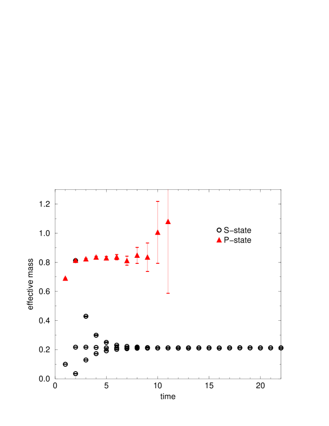
FIG. 1.: A representative effective mass plot for S- and P-states at $(\beta,\kappa,m_{Q})=(1.80,0.1409,6.00)$. One can clearly observe a plateau for long enough times. For the S-states we employed 3 different smearings, which result in different overlaps with the ground state.

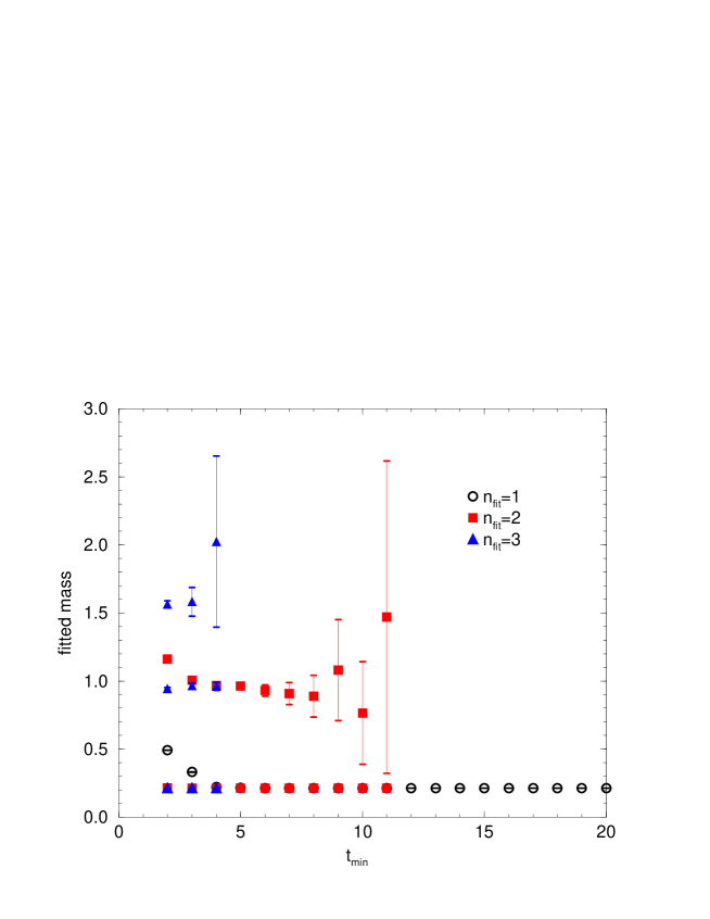
FIG. 2.: Here we show consistent fit results for the S-state of Fig. 1 when plotted against the start of the fit range, $t_{min}$. We fixed $t_{max}=24$ throughout. Different symbols denote different values for $n_{\rm fit}$ in the multi-exponential fit of Eq. 15.

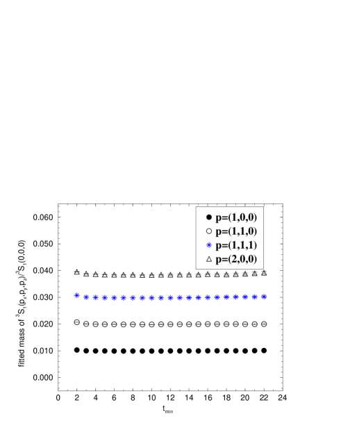
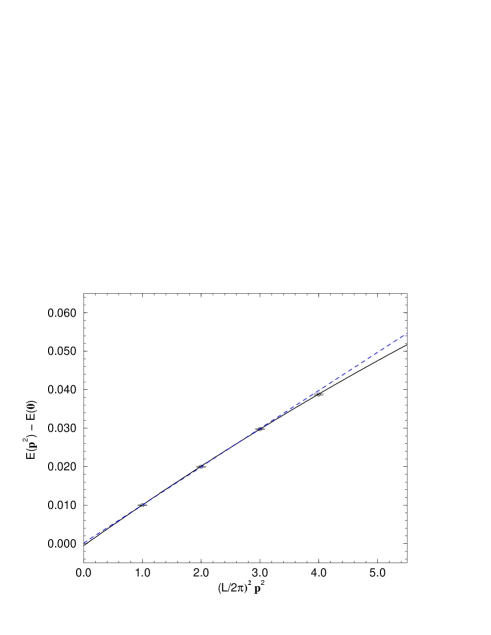
FIG. 3.: These figures illustrate the tuning of the quark mass as described in the main text. On the left-hand side we show the $t_{min}$-plots for the ratio fits of different momentum states with respect to the ${{}^{3}}S_{1}$ at rest. We can perform two consistent fits up to ${\bf p}^{2}$ (dashed line) and up to ${\bf p}^{4}$ (solid line) in the dispersion relation, Eq. 17.

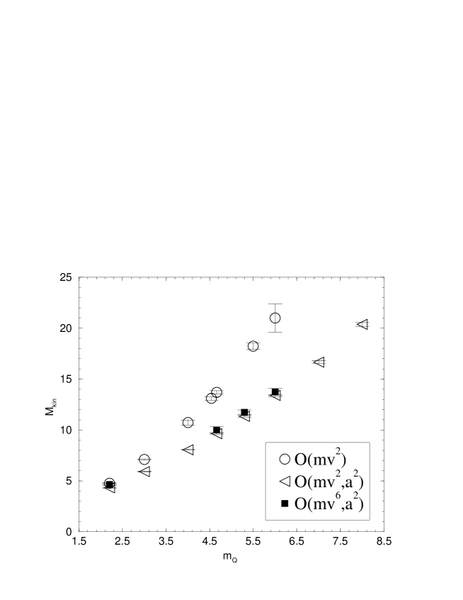
FIG. 4.: Quark mass dependence of $M_{\rm kin}$. Here we can see sizeable discretisation errors for almost the whole range of quark masses between charm and bottom at $(\beta,\kappa)=(1.80,0.1409)$. The implementation of $O(a^{2})$ improvement in the NRQCD approach is clearly important on our lattices. In contrast, the sensitivity of $M_{\rm kin}$ to the relativistic correction terms is much smaller.

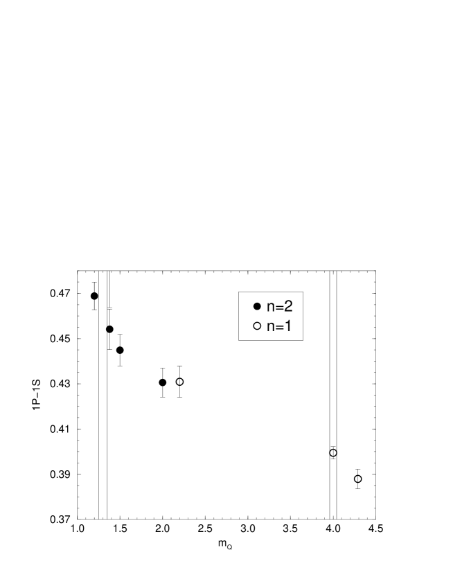
FIG. 5.: Heavy quark mass dependence of the $1P-1S$ splitting. We plot the (1P-1S) splitting against the heavy quark mass at $(\beta,\kappa)=(1.95,0.1375)$ and with two value of the stability parameter, $n=1,2$. The vertical lines denote the regions of the charmonium and bottomonium system.

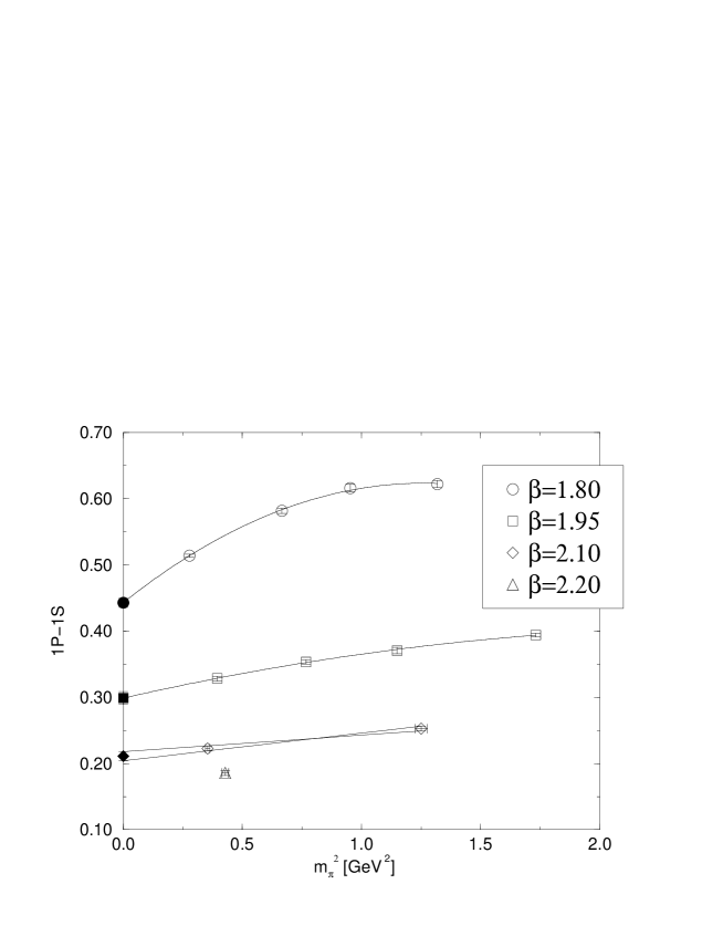
FIG. 6.: Light quark mass dependence of $1P-1S$ splitting in Bottomonium. We use quadratic fits in $m_{\pi}^{2}$ to extrapolate our data from four different sea quark masses to the chiral limit. For the two sea quark masses at $\beta=2.10$ we show an estimate of the chiral limit by drawing straight lines. The single point at $(\beta,\kappa)=(2.20,0.1368)$ is shown for completeness.

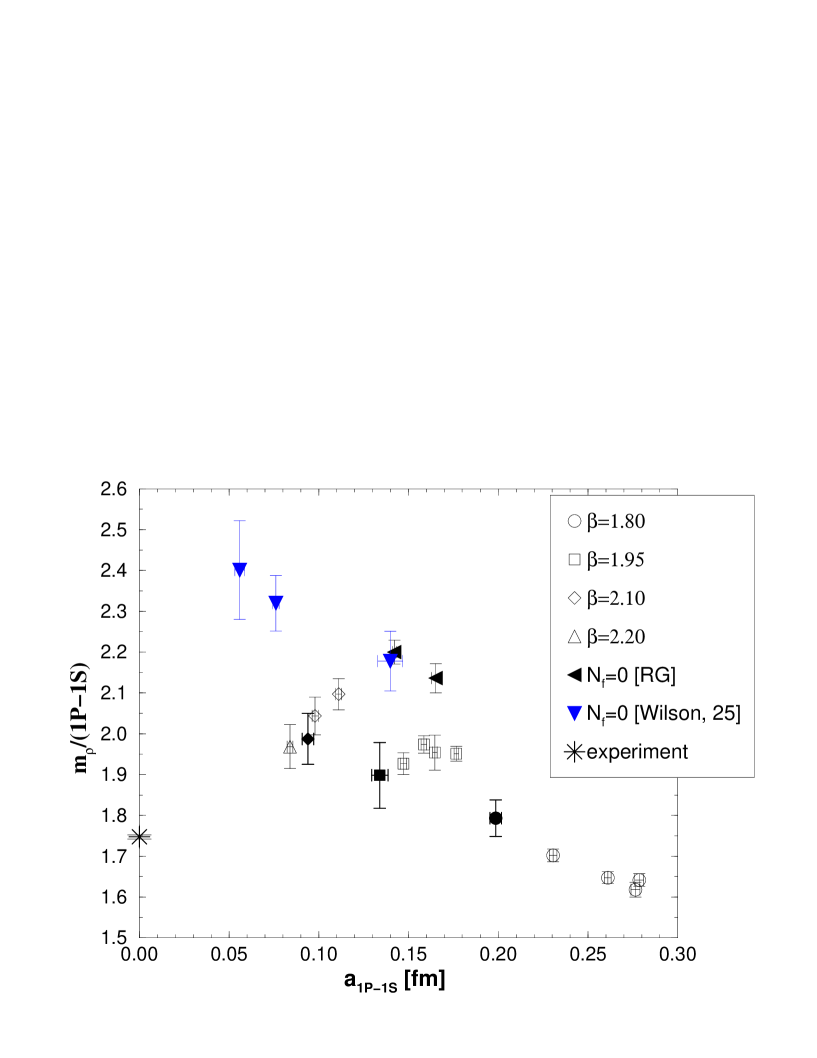
FIG. 7.: Here we show the ratio $m_{\rho}/(1P-1S)$, where scaling violations can be seen. In each case we use open symbols to denote data from dynamical calculations with different sea quark mass and full symbols to mark the chirally extrapolated values. Representative quenched results are also shown as full symbols.

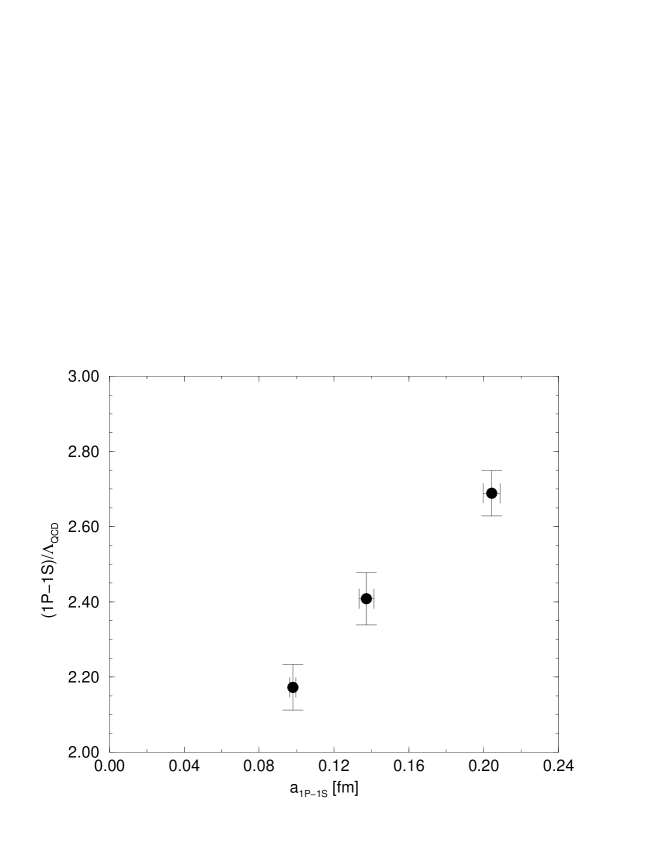
FIG. 8.: Asymptotic scaling. In this plot we take the chirally extrapolated values for $1P-1S$ and compare their scaling behaviour with respect to $\Lambda_{\rm QCD}$. The latter is taken from 2-loop perturbation theory.

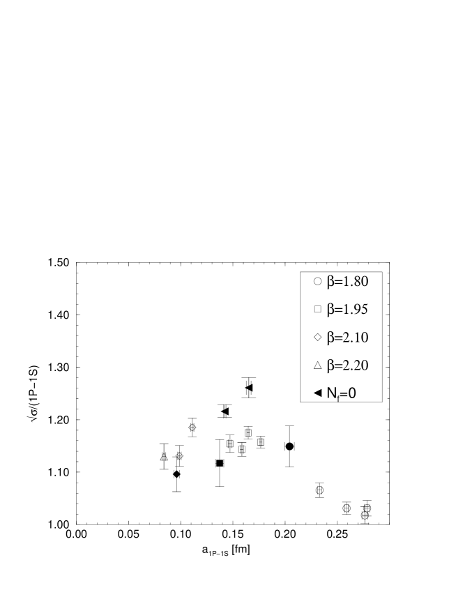
FIG. 9.: In contrast to Figs. 7 and 8, we observe a better scaling for the ratio $\sqrt{\sigma}/(1P-1S)$ on our finer lattices.

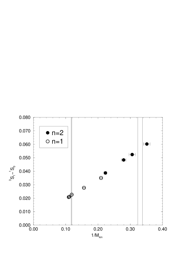
FIG. 10.: Mass dependence of hyperfine splitting. Here we show the strong mass-dependence of the hyperfine splitting, ${{}^{3}}S_{1}-{{}^{1}}S_{0}$, plotted against the inverse kinetic mass at $(\beta,\kappa)=(1.95,0.1375)$. The vertical lines denote the regions of the bottomonium and charmonium system. This splitting is clearly very sensitive to the parameters of NRQCD. All data points are from updates with $O(mv^{6},a^{2})$ and $n=1,2$ denotes different values of the stability parameter.

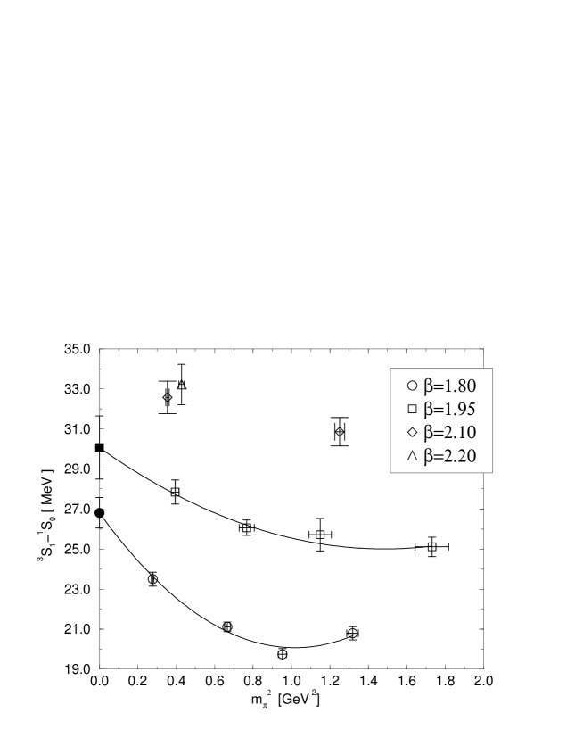
FIG. 11.: Hyperfine splitting vs. $m_{\pi}^{2}$. Here we collect the data for the the ${{}^{3}}S_{1}-{{}^{1}}S_{0}$ splitting in bottomonium from all values of $(\beta,\kappa)$. A clear dependence on the sea quark mass can be seen. The linear-plus-quadratic fit curves are shown as solid lines. Here we used the $1P-1S$ splitting to determine the lattice spacing.

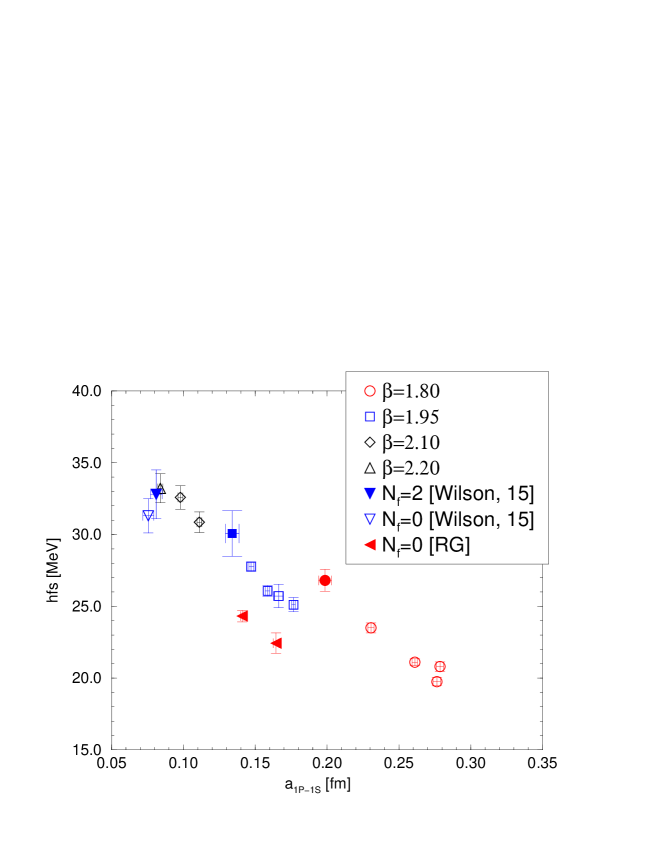
FIG. 12.: Scaling violations for hyperfine splitting. Open symbols correspond to runs with different sea quark mass. Filled symbols denote the dynamical data after chiral extrapolation and results with $N_{f}=0$. We used $1P-1S$ splitting to determine the lattice spacing.

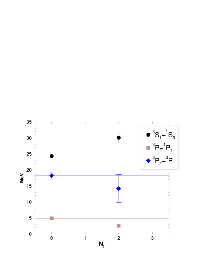
FIG. 13.: Direct comparison of the bottomonium spin structure for quenched and full QCD at the same lattice spacing of $a\approx 0.14$ fm. The $N_{f}=2$ data is taken from the chiral limit of our measurements at $\beta=1.95$.

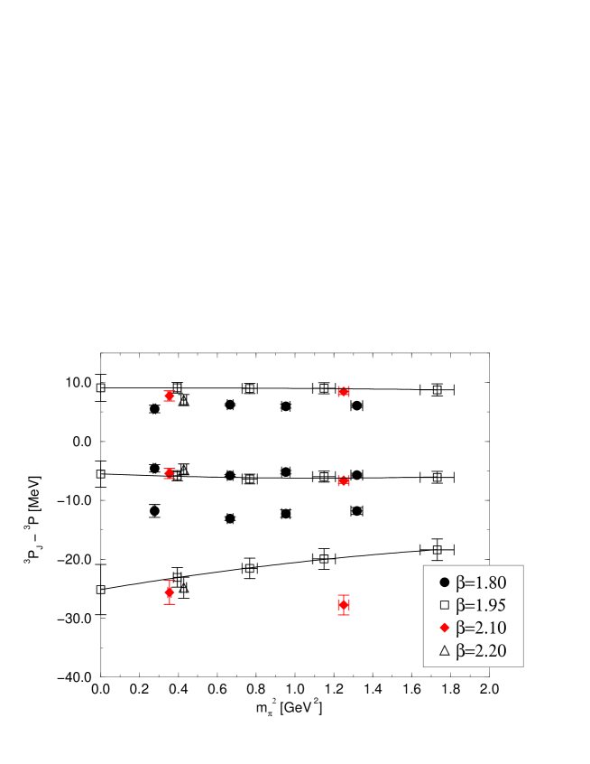
FIG. 14.: Fine structure in Bottomonium. Here we plot (top to bottom) ${{}^{3}}P_{2},{{}^{3}}P_{1}$ and ${{}^{3}}P_{0}$ relative to the spin averaged triplet state: ${{}^{3}}P\equiv 1/9(5{{}^{3}}P_{2}+3{{}^{3}}P_{1}+1{{}^{3}}P_{0})$. The corresponding experimental values are: 13 MeV, -8 MeV and -40 MeV.

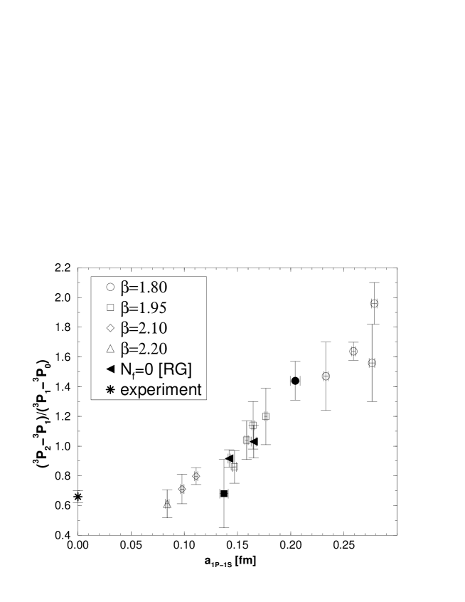
FIG. 15.: Fine structure ratio in Bottomonium. Here the lattice data should be compared to the experimental value of 0.66(4). It is apparent that there are still large underlying scaling violations, but no clear sea quark dependence.

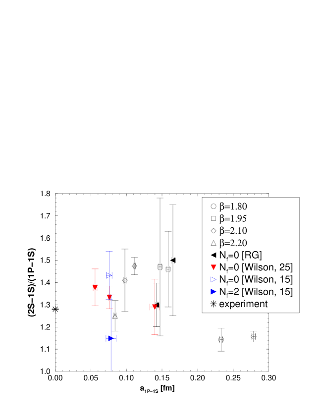
FIG. 16.: Here we show a scaling plot of the ratio $R_{2S}=(2S-1S)/(1P-1S)$. It is apparent that one needs much smaller statistical errors to resolve any systematic effects. We show our results from different sea quark masses along with representative results from other collaborations.

REFERENCES

- [1] S. Aoki al., CP-PACS Collaboration, Phys.Rev.Lett.84 (2000) 238.
-
[2]
R. Burkhalter (CP-PACS Collaboration),
Nucl.Phys.B(Proc.Suppl.)73 (1999) 3;
S. Aoki et al., CP-PACS Collaboration, Nucl.Phys. B (Proc. Suppl.) 73 (1999) 192;
A. Ali Khan et al., CP-PACS Collaboration, hep-lat/9909050 and hep-lat/0004010. - [3] S. Aoki et al., (CP-PACS Collaboration), Nucl.Phys.(Proc.Suppl.) 73 (1999) 216.
- [4] K.G. Wilson, Phys.Rev. D10 (1974) 2445; E. Eichten and F.L. Feinberg, Phys.Rev.Lett.43 (1979) 1205; Phys.Rev.D23 (1981) 2724.
- [5] M. Neubert, Phys.Rept.245 (1994) 259; and references therein.
- [6] B. Thacker and G. P. Lepage, Phys.Rev.D 43 (1991) 196.
- [7] A.X. El-Khadra et al., Phys.Rev.D55 (1997) 3933.
- [8] C.T.H. Davies and B. Thacker, Nucl.Phys. B 405 (1993) 593; C.T.H. Davies et al., Phys.Rev.D50 (1994) 6963.
- [9] G. P. Lepage et al., Phys.Rev.D46 (1992) 4052;
- [10] C. J. Morningstar, Phys.Rev.D48 (1993) 2265.
- [11] T. Manke et al., Phys.Lett.B408 (1997) 308.
- [12] C.T.H. Davies et al., Phys.Rev.D52 (1995) 6519.
- [13] H.D. Trottier, Phys.Rev.D55 (1997) 6844.
- [14] C.T.H.Davies et al., Phys. Lett.B345 (1995) 42; Phys.Rev.D56 (1997) 2755.
- [15] N. Eicker et al., Phys.Rev.D57 (1998) 4080.
- [16] Y. Iwasaki et al., Nucl.Phys.B258 (1985) 141; UTHEP-118 (Tsukuba, 1993).
- [17] B. Sheikholeslami and R. Wohlert, Nucl.Phys.B259 (1985) 572.
- [18] G. P. Lepage and P.B. Mackenzie, Phys.Rev.D48 (1993) 2250.
- [19] S. Aoki et al., Phys.Rev.D58 (1998) 074505; S. Aoki et al., Nucl.Phys.B540 (1999) 501.
- [20] T. Manke et al., CP-PACS Collaboration, Phys.Rev.Lett.82 (1999) 4396.
- [21] P. Lepage, Nucl.Phys.B60A (1998) 267.
- [22] J.E. Mandula et al., Nucl.Phys.B228 (1983) 91.
- [23] W.H. Press et al., “Numerical recipes in Fortran”, (2nd Edition), Cambridge University Press (1992).
- [24] U. Glässner et al., SESAM Collaboration, Phys.Lett.B383 (1996) 98.
- [25] C.T.H. Davies, et al., Phys.Rev.D58 (1998) 054505.
- [26] J. Pantaleone and S.-H.H. Tye, Phys.Rev.D37 (1998) 3337.