Green’s Function Monte Carlo study of correlation functions in the (2+1)D lattice gauge theory
Abstract
A “forward walking” Quantum Monte Carlo (QMC) algorithm has been developed to calculate correlation functions for the Hamiltonian lattice formulation of Yang-Mills theory in (2+1) dimensions. It is shown that Wilson loops can be calculated with high accuracy. Creutz ratios are used to determine the string tension, which agrees with results from other approaches. Timelike correlations are used to estimate the mass gaps, which agree with series expansion results in the strong coupling regime.
I Introduction
The two major variants of lattice gauge theory (LGT) are the “Euclidean” formulation of Wilson [2], and the “Hamiltonian” version of Kogut and Susskind [3]. In the Euclidean régime, classical Monte Carlo simulations have proved to be extremely powerful in extracting quantitative predictions from the theory, as first shown by Creutz [4]. This approach is preferred by an overwhelming majority of lattice gauge theorists at the present time.
The Hamiltonian formulation is still worthy of study, however. It can provide a valuable check of universality, for instance. Lattice gauge theory relies on the fundamental assumption that quantities such as mass ratios calculated in the continuum limit (a critical point of the lattice model) must be ‘universal’, i.e. independent of the microscopic lattice structure or space-time formulation. There is not much real doubt that this is correct, but it is important to provide checks where possible [5]. Another reason is that many techniques imported from quantum many-body theory and condensed matter physics can be employed in this arena, which may give useful results. Examples include the strong-coupling series approach [6], the -expansion [7], the coupled-cluster method [8, 9], and others. Nevertheless, it seems likely that Monte Carlo simulations will provide the most robust and accurate numerical techniques in this area also. Our aim in this paper is to discuss some further applications of these Quantum Monte Carlo methods [10].
The use of quantum Monte Carlo methods in Hamiltonian LGT has a long and somewhat chequered history, and lags a good ten years behind the Euclidean developments. The first calculations used a strong-coupling basis involving discrete “electric field” link variables, and a “Projector Monte Carlo” approach [11, 12], which used the Hamiltonian itself to project out the ground state. A later version of this was the “stochastic truncation” approach of Allton et al. [13]. Using this approach one can successfully compute string tensions and mass gaps for Abelian models [14]. For non-Abelian models, however, some problems arose [14]. Using an electric field representation for the link variables and a Robson-Webber recoupling scheme [15] at the vertices requires the use of Clebsch-Gordan coefficients or 6-symbols, which are not known to high order for ; and furthermore, the ‘minus sign’ problem rears its head, in that destructive interference occurs between different paths to the same final state. It may well be that a better choice of strong-coupling basis, such as the ‘loop representation’, might avoid these problems; but this has not yet been demonstrated.
Heys and Stump [16] and Chin et al. [17] pioneered the use of “Greens Function Monte Carlo” (GFMC) or “Diffusion Monte Carlo” techniques in Hamiltonian LGT, in conjunction with a weak-coupling representation involving continuous gauge field link variables. This was successfully adapted to non-Abelian Yang-Mills theories [18], with no minus sign problem arising. In this representation, however, one is simulating the wave function in gauge field configuration space by a discrete ensemble or density of random walkers: it is not possible to determine the derivatives of the gauge fields for each configuration, or to enforce Gauss’s law explicitly, and the ensemble always relaxes back to the ground state sector. Hence one cannot compute the string tensions and mass gaps directly as Hamiltonian eigenvalues corresponding to ground states in different sectors, as one does in the strong-coupling representation. Chin, Long and Robson [19] thus resorted to “variational Monte Carlo” (VMC) techniques to compute mass gaps. They obtained some reasonable results; but this approach always suffers from the major drawback that there is an unknown systematic error in the results, due to their dependence on the form of the variational wave function which is chosen.
It appears, therefore, that to make unbiased measurements of mass gaps in the weak-coupling representation one is forced back to the more laborious approach used in Euclidean calculations: namely, to measure an appropriate correlation function, and estimate the mass gap as the inverse of the correlation length. In ref. [14] the GFMC method was tested on the (2+1)D U(1) model using a “secondary amplitude” technique to compute expectation values: but this proves to be expensive and prone to bias [20, 21]. In this paper we will show how the standard ‘forward-walking’ technique used in many-body theory [22] can be used for this purpose. The forward-walking method has already been applied to lattice spin models by Runge [23] and Samaras and Hamer [21]. Here we apply it to the compact Yang-Mills theory in (2+1) dimensions, which has been a standard test-bed for Hamiltonian LGT.
A brief discussion of the model is given in Section II. Our Monte Carlo methods are outlined in Section III. The GFMC method is briefly summarized, and then the forward-walking method for estimating expectation values is discussed, together with a technique for measuring timelike correlations. In Section IV the results are presented. Our conclusions are summarized in Section V.
II Model Hamiltonian
In a weak coupling basis the Hamiltonian for the compact LGT in (2+1)D is given by [3, 24]:
| (1) |
where is the gauge field variable on link and
| (2) |
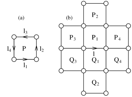
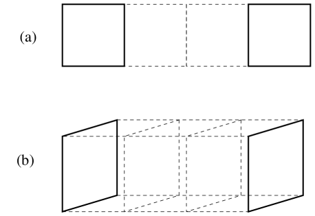
is the plaquette variable for a lattice plaquette , formed by the four links , as illustrated in Fig. 1(a). We consider a periodic, square lattice of linear dimension and lattice spacing . The ‘strong coupling’ parameter approaches infinity in the continuum limit .
This is an interesting model, which possesses some important similarities with QCD (for a more extensive review, see for example ref. [14]). If one takes the ‘naive’ continuum limit at a fixed energy scale, one regains the simple continuum theory of non-interacting photons [26]; but if one renormalizes or rescales in the standard way so as to maintain the mass gap constant, then one obtains a confining theory of free massive bosons, as discussed by Polyakov [27], and proven by Göpfert and Mack [28]. The Hamiltonian version of the model has been well studied by a variety of methods: some of the more recent include series expansions [29, 30], finite-lattice techniques [31], the -expansion [32, 33], and coupled-cluster techniques [34, 35, 36], as well as QMC [17, 37, 38, 14]. Quite accurate estimates have been obtained for the string tension and mass gaps, which can be used as comparisons for our Monte Carlo results. The finite-size scaling properties of the model can be predicted using an effective Lagrangian approach combined with a weak-coupling expansion [25], and the predictions agree very well with finite-lattice data [14].
III Monte Carlo Methods
A Greens Function Monte Carlo
We use the Green’s Function Monte Carlo [GFMC] method [10], which was adapted to the model by Heys and Stump [16], and Chin et al. [17]. A brief summary of the method can be given as follows.
In a weak-coupling representation, the basis states are taken to be eigenstates of the plaquette angles , which can take continuous values. The Hamiltonian (1) can be written as
| (3) |
where
| (4) |
and the plaquette angles and link angles are related by equation (2). The imaginary time Schrödinger equation for the system is
| (5) |
where is a trial energy, representing a constant shift in the zero of energy, which will prove useful. The imaginary time evolution operator acts as a projector onto the ground state :
| (6) |
for any trial state , provided that is not orthogonal to .
Equation (5) is a diffusion equation in configuration space, and is easily simulated by the Green’s Function Monte Carlo method. It is assumed that the ground-state wave function can be chosen positive everywhere, and it is simulated by the density distribution of an ensemble of random walkers in configuration space, with weights {}. The first term on the right of Eq. (5) produces diffusion, and is simulated by a Gaussian random walk of the members of the ensemble as time proceeds, while the term produces a growth or decay in the density which is simulated by a branching process.
B Variational Guidance
The efficiency and accuracy of the simulation are greatly enhanced by the use of variational guidance or importance sampling [10]. Let be a variational approximation to the true ground-state wave function, and define a new probability distribution
| (7) |
Then the modified imaginary time Schrödinger equation for reads
| (8) |
where
| (9) |
is the local energy obtained from the trial function, and
| (10) |
is a “quantum force” term, which produces a directed drift in the ensemble towards the configurations favoured by the trial wave function. By a good choice of and the “excess local energy” term can be made very small, which reduces the amount of branching necessary, and reduces the statistical fluctuations in the results.
For small time steps , an approximate Green’s function solution to Eq. (8) is
| (12) | |||||
In the Monte Carlo simulation, each iteration corresponds to a time step . At each iteration, we sweep through each link in turn, and simulate the corresponding exponential factor in the sum on the right of (12) by a random displacement of the link variable for each walker:
| (13) |
where is randomly chosen from a Gaussian distribution with standard deviation . The first term in (13) is the “drift” term, and the second is the “diffusion” term. The first exponential on the right of (12) is simulated by simply multiplying the “weight” of each walker by an equivalent amount.
At the end of each iteration, the trial energy is adjusted to compensate for any change in the total weight of all walkers in the ensemble; and a “branching” process is carried out, so that walkers with weight greater than (say) 2 are split into two new walkers, while any two walkers with weight less than (say) 1/2 are combined into one, chosen randomly according to weight from the originals. This procedure of “Runge smoothing” [23] maximizes statistical accuracy by keeping the weights of all the walkers within fixed bounds, while mimimizing any fluctuations in the total weight due to the branching process.
When equilibrium is reached after many sweeps through the lattice, the average value of the trial energy will give an estimate of the ground-state energy , and the weight density of the ensemble in configuration space will be proportional to . Various corrections due to the finite time interval have been ignored in this discussion, and the limit must be taken in some fashion to eliminate such corrections.
In the simulations presented here, a trial function for the ground state was chosen as
| (14) |
with two variational parameters and , where the sum over denotes a sum over nearest-neighbour pairs of plaquettes, forming rectangles ( Wilson loops) on the lattice. That is, the uncorrelated single plaquette trial function used in [14] has been extended to include a correlated term. In the single plaquette case () it is straightforward to determine the optimal value for [16]. For the correlated case (), the optimum values for and must be found by means of a separate Variational Monte Carlo (VMC) calculation, where the variational energy
| (15) |
is minimised. The procedure is described in [16] where a six- parameter variational wave function was used to estimate the mass gaps in the model at the VMC level. In short, one samples the local trial energy over configurations randomly generated by a Metropolis procedure, distributed with respect to the weight function . A downhill simplex method was used to perform the minimisation. To this end was evaluated in a region centered around a guessed minimum using the reweighting procedure described in [16], whereby uncorrelated configurations generated with respect to the weight function were reweighted to give a distribution corresponding to the required weight function for a pair in the neighbourhood of . This procedure was iterated until the minimum converged. We used 100,000 independent configurations on an lattice to determine . This allowed the optimal and to be fixed to within around 1%. Though it is possible to optimise and for each lattice size, for a given value of the coupling , we used the same values of and for all lattice sizes . The values of and used are listed in Table I.
The use of a correlated trial wave function is expected to markedly decrease the variance of estimators and the amount of branching in the population smoothing process, particularly in the physically interesting weak coupling regime ( large). Moreover, because the trial function is closer to the true ground state, fewer forward walking iterations (see section III C) are required in order to derive converged estimators for correlation functions. These advantages come at a price in that updating of GFMC configurations becomes more complicated: The local trial energy is
| (16) |
and the quantum force term is given by
| (18) | |||||
Here, ,…, and ,…, denote the 4 closest plaquettes on either side of the link , as illustrated in Fig. 1(b). These expressions are more difficult to compute than in the single parameter () case. However, the increased complexity is easily offset by the gains from variance reduction.
C Forward-walking method
The quickest method of estimating an expectation value is simply to form the weighted average of over the ensemble of random walkers (we assume Q is diagonal in the chosen basis, for simplicity). This produces an estimate according to the distribution , rather than . The estimate can be perturbatively improved [10], but there remains an unknown systematic error due to the dependence on the trial function . For this reason, we have preferred to use the so-called “forward-walking” method for estimating expectation values.
The forward-walking method is a robust technique for estimating expectation values [22, 39, 40], based on the following equation [23] for an operator :
| (19) | |||||
| (20) | |||||
| (21) |
where is the evolution operator for time , and is the same operator in the similarity transformed basis. Again we have assumed that the operator is diagonal in the basis of plaquette variables .
This equation is implemented by [22, 39, 40] the following procedure:
-
i)
Starting from the trial state, iterate until equilibrium is achieved, then begin a measurement;
-
ii)
Record the value for each walker (“ancestor”) at the beginning of the measurement;
-
iii)
Propagate the ensemble as normal for iterations, keeping a record of the “ancestor” of each walker in the current population;
-
iv)
Take the weighted average of the with respect to the weights of the descendants of after the iterations, using sufficient iterations that the estimate reaches a ‘plateau’.
This procedure has been tested for the magnetization in the 2D lattice Heisenberg model by Runge [23], and for correlation functions in the 1D transverse Ising model by Samaras and Hamer [21], and works very well. The drawback to the procedure is that after a large number of iterations many of the “ancestors” will die out, leaving no descendants, which leads to a progressive loss of statistical accuracy. Thus it is even more crucial in this connection to use a good guiding wavefunction so as to minimize “branching”.
D Timelike Correlations
In order to estimate mass gaps in this model, we have again used the forward-walking technique to measure correlations between operators at different times. The mass gaps can then be estimated from the decay constants for these correlation functions.
A timelike correlator can be found from the following equations:
| (22) |
| (23) |
| (24) |
where . This can be implemented in much the same way as an expectation value (assuming both and are diagonal in the weak-coupling representation). At the beginning of the measurement, record the ‘ancestor’ configurations as in Sec. (III C). Then allow the ensemble to propagate for time , with the branching process turned off so that each state retains its identity. At the end of time , record the initial value and the final value . Propagate each state for a further iterations as before, and then average, weighting each ‘ancestor’ state according to the forward-walking prescription of Sec. (III C).
IV Results
Simulations were carried out for lattices up to sites, using runs of 10,000 walkers over 50,000 iterations. At each iteration several sweeps of the lattice were performed, after which Runge smoothing (the branching (combining) of high (low) weight walkers) was imposed on the walker population. The average percentage of walkers branched/combined per iteration depends on a number of factors: clearly, the time step and number of lattice sweeps performed per iteration can be adjusted in order to control the extent of the branching. We wish to choose values of which are sufficiently small that time discretization errors can be made negligible. Furthermore, the number of sweeps performed per iteration was chosen so that essentially uncorrelated measurements could be made roughly every 150 iterations. We found that, for the lattice sizes and couplings considered, this could be achieved in such a way that on average no more than 10% of the walkers were branched/combined per iteration. However, the extent of the smoothing per iteration depends on the quality of the variational guiding function. Generally, the two-parameter guiding function (14) works better for smaller couplings and smaller lattice sizes . Under the most strained conditions considered (, ) around 10% of the walkers were branched/combined per iteration for the values of chosen and the number of sweeps per iteration required to get independent measurements, whereas for the ratio was a fraction of a percent. The first 2000 iterations were discarded to allow for equilibration. Two values of the time step were used, differing by a factor of 5 (e.g. and ). The number of sweeps performed for the smaller value was 5 times as large as that for the larger value and as a result measurements were equally uncorrelated in the two cases. The typical number of sweeps used per iteration, e.g. for and was 1 and 5 respectively. Linear extrapolations were made to the limit . The linear dependence on has been checked previously [14].
A Ground-state Energy
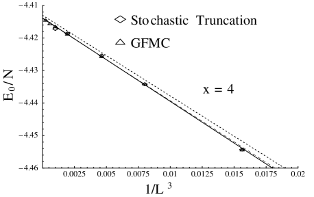
Results for the ground-state energy per site at coupling are graphed against in Fig. 2. They agree within errors with those of the earlier study [14] up to , and extend them to . It can be seen that the data are fitted quite well by the form
| (25) |
which compares very well with effective Lagrangian theory and the weak-coupling series prediction [25, 14]
| (26) |
The estimated bulk value compares well with estimates of from strong-coupling series [29], from a -expansion [30], and from the coupled cluster method (CCM) [9].
B Wilson Loops
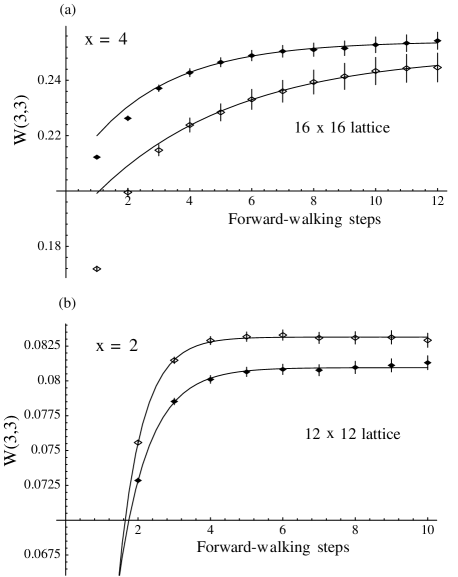
The expectation values of Wilson loops were computed using the forward-walking method outlined in section III C. Measurements of the observables were made in cycles starting around every 150 iterations, with typically 10 forward-walking weighted averages over the ensemble taken at time steps of 12–15 iterations. For each time step the weighted averages were then block averaged over successive measurement cycles. Fig. 3(a) shows the forward-walking convergence of the Wilson loop measured on the lattice at coupling for a trial run involving 1200 walkers, 20,000 iterations, a time step , 3 sweeps of the lattice per iteration, with 12 forward-walking weighted averages being taken every 20 iterations in measurement cycles made 250 iterations apart. Results are shown for two different guiding functions, using the 1-parameter and 2-parameter forms respectively. It can be seen that in both cases the data relax exponentially towards a common equilibrium value, which can be estimated by making an exponential fit to the data. The equilibrium value is then taken as the final result for the Wilson loop. It can also be seen that the 2-parameter form reduces the variance and produces much more rapid convergence to the asymptotic value.
Typical results from a production run (using the 2-parameter guiding function) are shown in Fig. 3(b). In this case , and 50,000 iterations are performed with 10,000 walkers. Measurement cycles involving 10 forward-walking weighted averages 16 iterations apart were started every 165 iterations. Results for two values of (0.05 and 0.01), using 1 and 5 lattice sweeps per iterations respectively, are shown.
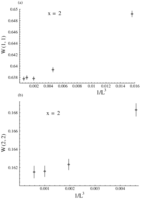
Fig. 4 displays the values for the ‘mean plaquette’ at coupling , graphed against . There is evidently a discrepancy here between our present results and those of [14], obtained using the secondary amplitude technique. Either the errors in [14] have been underestimated for the larger lattices and couplings, or the discrepancy could have arisen from bias in the secondary amplitude technique [20, 21]. Our present results show a consistent finite-size scaling behaviour for :
| (27) |
to be compared with the weak-coupling series prediction [25]
| (28) | |||||
| (29) |
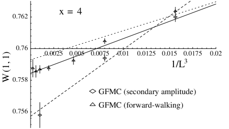
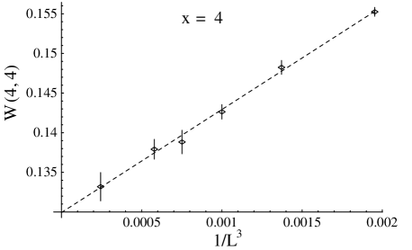
obtained using the Hellmann-Feynman theorem. The agreement is once again quite good. Extrapolation to the axis gives a bulk limit of , to be compared with strong-coupling series [29] 0.80(3), the -expansion [33] 0.757(4), and the CCM [9] 0.7585. The results for other Wilson loops scale similarly with lattice size. For example, the finite-size scaling of the Wilson loop is shown in Fig. 5.
Of course, because the model has a gap for any finite value of , one should expect to see a crossover from this algebraic (free-photon theory) scaling to exponential convergence for large enough . Indeed, for smaller values of the coupling, exponential scaling sets in rapidly enough that essentially bulk results can be obtained on relatively small lattices. This is illustrated in Fig. 6 in the case where we see a definite crossover from algebraic to exponential scaling for the mean plaquette and the Wilson loop when reaches around 10.
Table II lists the final estimates we have obtained for the bulk ground-state energy per site and Wilson loop values at some selected couplings.
C String Tension
In a confining model, the Wilson loops are expected to behave asymptotically as
| (30) |
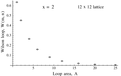
where is the area of the loop and is the string tension. In Fig. 7 we illustrate this behaviour for the case on the lattice by plotting the Wilson loops and as a function of area. The standard estimator of the string tension is the Creutz ratio
| (31) |
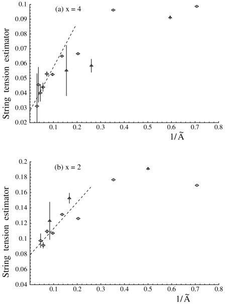
Fig. 8(a) shows the Creutz ratios graphed against (where is the average area of the loops used to form the ratio) at , from which we obtain the rough estimate
| (32) |
Because the Creutz ratios decrease very rapidly with , and the relative error correspondingly increases, it is very difficult to determine a reliable value for the string tension. Given the limited number of data points, it is probably more fruitful to use a two-point estimator
| (33) |
formed from successive pairs of Wilson loops. Included in Fig. 8(a) are plots of these estimators against . Unfortunately, the two-point estimators display oscillations (which the Creutz ratios were designed to eliminate) so it is again difficult to perform a linear extrapolation to obtain an estimate of the string tension. Nevertheless, a linear fit through the points gives an estimate of the string tension of , somewhat lower than the result above.
We have performed a similar analysis for , working with the lattice which is sufficiently close to the bulk limit. The results for the string tension estimators are shown in Fig. 8(b). In this case a linear extrapolation of the two-point estimators yields an estimate of for the string tension.
The string tension has previously been calculated as an energy per unit length, . The best available values at are from stochastic truncation [14], and from an ‘exact linked cluster expansion’ [41]. The quantities are related by
| (34) |
where is the speed of light, estimated as at from the weak-coupling expansion [25]. Hence corresponds to . This is in rough agreement with the result above.
We also attempted the analysis for smaller values of . However, because the Wilson loops decay extremely rapidly in these cases, it is not possible to obtain enough data points to make sensible extrapolations.
D Mass Gaps
We have attempted to estimate mass gaps from the exponential decay of correlation functions, as is done in the Euclidean approach. The lowest-lying excitations in the strong-coupling limit are the single-plaquette excitations, antisymmetric or symmetric under reflections respectively. At first we attempted to use the spatial correlations between plaquette operators for this purpose; but the signal from the connected spatial correlations turns out to be very small, and can even change sign, giving no good exponential decay signal. We can understand this problem as follows: : we are restricted to a plane in the spatial directions, and can therefore only measure correlations between plaquette operators “edge on” to each other, as illustrated in Fig. 9(a), as opposed to the “face on” configuration in Fig. 9(b). This means there is very poor overlap with the configurations of interest in the intermediate state.
We are thus compelled to fall back on the correlations in imaginary time , which do correspond to “face on” plaquettes as in Fig. 9(b). Using the method of III D, we have measured correlation functions
| (35) |
where the plaquette operators have been summed over all positions to project out the zero-momentum intermediate states, and the sums are either symmetric or antisymmetric under reflections.
As with the Wilson loop calculations, typically 50,000 iterations were performed with 10,000 walkers and forward-walking measurment cycles were started every 150 iterations. As mentioned, at the start of each measurement cycle, Runge smoothing was switched off so that no walkers were created or destroyed while timelike correlation functions were calculated. Between 10 and 20 timelike correlations (between the plaquette operators at the start of the measurement cycle and later times )were measured at intervals of one or two iterations. For each of the timelike measurements the “physical time” is given by:
where is the basic timestep, is the number of sweeps of the lattice and denotes the number of iterations between the calculation of initial and final plaquette operators.
At this point Runge smoothing was switched on again and forward-walking weighted averages of the timelike correlations were calculated over most of the measurement cycle at intervals of 10–20 iterations. Again the weighted averages were block averaged over all measurement cycles, and exponential fitting was used to find the forward-walking relaxed estimates of the timelike correlation functions. As with the Wilson loops, two values of the time step were used and linear extrapolation was used to obtain estimates of the correlators. Again, the two values of used differed by a factor of 5, and 5 times as many lattice sweeps were performed per iteration for the smaller so that the “physical” times over which the correlations were measured were the same (i.e. was kept fixed).
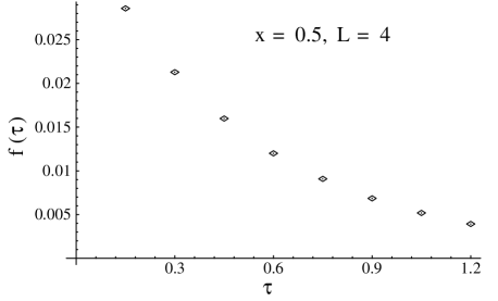
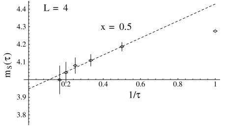
A typical plot of the resulting estimates for the timelike correlation function , as a function of , is shown in Fig. 10 for the antisymmetric correlator with and . It can be seen that shows a smooth exponential decay with . Defining an ‘effective mass’ for each pair of points by
| (36) |
one finds that the effective mass decreases somewhat with , as might be expected. An ad hoc fit in , illustrated in Fig. 11, gives a final estimate for the mass of the corresponding intermediate state. These values are listed as a function of lattice size in Table III for couplings , 1 and 2. For the higher couplings the exponential decay is so slow that we have been unable to obtain useful results for the mass. To do so would require measurements to be made over substantially larger time scales with significantly greater accuracy. Unfortunately, our results were not sufficiently accurate to sensibly resolve the form of the lattice size dependence for the couplings studied. In Table III we list results of estimates of the bulk mass from other sources. It can be seen that for the couplings considered, the agreement between methods is reasonable.
V Summary and Conclusions
In this paper we have shown how the standard ‘forward-walking’ methods of quantum many-body theory [10] can be used to calculate expectation values and correlation functions in Hamiltonian lattice gauge theory. Accurate values for the Wilson loops have been obtained, and their finite-size scaling behaviour has been demonstrated. The string tension can then be estimated using two-point and Creutz ratios. The Wilson loop values dropped away too quickly with lattice size to give accurate string tensions at small couplings ; but this problem could presumably be rectified by looking at timelike correlators—either timelike Wilson loops, or timelike correlations between Polyakov loops.
We have also shown how mass gaps can be estimated from the exponential decay of timelike correlators. This approach is very reminiscent of the techniques used in the Euclidean regime: our freedom of choice of the timelike measurement interval is akin to the choice of an anisotropic lattice in the ‘timelike’ direction in the Euclidean case. Reasonable results have been obtained for the masses at small couplings , but not at large .
The accuracy of the final results for the string tension and mass gaps is not remarkable; but it must be recalled that this is the first time that unbiased estimates have been obtained for these quantities using a ‘weak-coupling’ representation and GFMC techniques. There are no doubt many ways by which the results could be improved: for example, by the use of improved guiding wavefunctions, or improved (“fuzzed”) correlation functions, or improved Hamiltonian operators. Our aim here has been to ‘prove the concept’, that forward-walking techniques can give reliable estimates for the correlation functions. In future work we plan to apply similar methods to the (3+1)D Yang-Mills theory.
Acknowledgments
This work is supported by the Australian Research Council. Calculations were performed on the SGI Power Challenge Facility at the New South Wales Center for Parellel Computing and the Fujitsu VPP300 vector machine at the Australian National Universtiy Supercomputing Facility.
REFERENCES
- [1] Email address: cjh@newt.phys.unsw.edu.au
- [2] K. G. Wilson, Phys. Rev. D 10, 2445 (1974).
- [3] J. Kogut and L. Susskind, Phys. Rev. D 11, 395 (1975).
- [4] M. Creutz, Phys. Rev. Lett. 43, 553 (1979).
- [5] C. J. Hamer, M. Sheppeard, W. H. Zheng and D. Schütte, Phys. Rev. D 54, 2395 (1996).
- [6] T. Banks, S. Raby, L. Susskind, J. Kogut, D. R. T. Jones, P. N. Scharbach and D. K. Sinclair, Phys. Rev. D 15, 1111 (1977).
- [7] D. Horn and M. Weinstein, Phys. Rev. D 30, 1256 (1984).
- [8] Guo Shuohong, Zheng Weihong and Liu Jiunmin, Phys. Rev. D 38, 2591 (1988).
- [9] R. F. Bishop, A. S. Kendall, L. Y. Wong and Y. Xian, Phys. Rev. D bf 48, 887 (1993); S. J. Baker, R. F. Bishop and N. J. Davidson, Phys. Rev. D 53, 2610 (1996); Nuc. Phys. B (Proc. Suppl.) 53, 834 (1997); Int. J. Mod. Phys., to appear;
- [10] D. M. Ceperley and M. H. Kalos, in Monte Carlo Methods in Statistical Mechanics, ed. K. Binder (Springer-Verlag, New York, 1979).
- [11] D. Blankenbecler and R. L. Sugar, Phys. Rev. D 27, 1304 (1983).
- [12] T. A. DeGrand and J. Potvin, Phys. Rev. D 31, 871 (1985).
- [13] C. R. Allton, C. M. Yung and C. J. Hamer, Phys. Rev. D 39, 3772 (1989).
- [14] C. J. Hamer, K. C. Wang and P. F. Price, Phys. Rev. D 50, 4693 (1994).
- [15] D. Robson and D. M. Webber, Z. Phys, C, 15, 199 (1982).
- [16] D. W. Heys and D. R. Stump, Phys. Rev. D 28, 2067 (1983).
- [17] S. A. Chin, J. W. Negele and S. E. Koonin, Ann. Phys. (N.Y.) 157, 140 (1984).
- [18] D. W. Heys and D. R. Stump, Phys. Rev. D 30, 1315 (1984); S. A. Chin, O. S. van Roosmalen, E. A. Umland and S. E. Koonin, Phys. Rev. D 31, 3201 (1985).
- [19] S. A. Chin, C. Long and D. Robson, Phys. Rev. Lett. 57, 60 (1986); Phys. Rev. Lett. 60, 1467 (1988); C. Long, D. Robson and S. A. Chin, Phys. Rev. D 37, 3006 (1988); D. W. Heys and D. R. Stump, Nuc. Phys. B 257, 19 (1985); Nuc. Phys. B 285, 13 (1987).
- [20] C. J. Hamer, M. Sheppeard and Z. Weihong, J. Phys. G 22, 1303 (1996).
- [21] M. Samaras and C. J. Hamer, Preprint.
- [22] M. H. Kalos, J. Comp. Phys. 1, 257 (1966).
- [23] K. J. Runge, Phys. Rev. B 45, 7229 (1992).
- [24] S. D. Drell, H. R. Quinn, B. Svetitsky and M. Weinstein, Phys. Rev. bf 19, 619 (1979).
- [25] C. J. Hamer and Zheng Weihong, Phys. Rev. D 48, 4435 (1993).
- [26] L. Gross, Commun. Math. Phys. 92, 137 (1983).
- [27] A. M. Polyakov, Phys. Lett. B 72, 477 (1978).
- [28] M. Göpfert and G. Mack, Commun. Math. Phys. 82, 545 (1982).
- [29] C. J. Hamer, J. Oitmaa, and Zheng Weihong, Phys. Rev. D 45, 4652 (1992).
- [30] C. J. Hamer, Zheng Weihong and J. Oitmaa, Phys. Rev. D 53, 1429 (1996).
- [31] A. C. Irving, J. F. Owens and C. J. Hamer, Phys. Rev. D 28, 2059 (1983).
- [32] D. Horn, G. Lana and D. Schreiber, Phys. Rev. D 36, 3218 (1987).
- [33] C. J. Morningstar, Phys. Rev. D 46, 824 (1992).
- [34] A. Dabringhaus, M. L. Ristig and J. W. Clark, Phys. Rev. D 43, 1978 (1991).
- [35] X. Y. Fang, J. M. Liu and S. H. Guo, Phys. Rev. D 53, 1523 (1996).
- [36] S.J. Baker, R.F. Bishop and N.J. Davidson, Phys. Rev. D53, 2610 (1996)
- [37] S. E. Koonin, E. A. Umland and M. R. Zirnbauer, Phys. Rev. D 33, 1795 (1986).
- [38] C. M. Yung, C. R. Allton and C. J. Hamer, Phys. Rev. D 33, 1795 (1986).
- [39] K. S. Liu, M. H. Kalos and G. V. Chester, Phys. Rev. B 10, 303 (1974).
- [40] P. A. Whitlock, D. M. Ceperley, G. V. Chester and M. H. Kalos, Phys. Rev. B 19, 5598 (1979).
- [41] A.C. Irving and C.J. Hamer, Nucl.Phys. B235, 358 (1984)
- [42] R. F. Bishop, private communication.
| 0.5 | 0.239 | 0.0088 |
|---|---|---|
| 1 | 0.409 | 0.033 |
| 2 | 0.585 | 0.089 |
| 4 | 0.771 | 0.150 |
| 0.4337(1) | 0.43350(7) | 0.43346(6) | |
| 0.2161(1) | 0.21526(7) | 0.21521(6) | |
| 0.0649(1) | 0.06377(7) | 0.06369(6) | |
| — | 0.01946(5) | 0.01927(4) | |
| — | 0.00391(5) | 0.00378(5) | |
| — | — | 0.00077(3) |
| 0.6492(3) | 0.6394(2) | 0.6378(2) | 0.6380(2) | 0.6378(2) | |
| 0.4772(3) | 0.4572(2) | 0.4544(2) | 0.4545(2) | 0.4545(2) | |
| 0.3134(3) | 0.2726(2) | 0.2675(2) | 0.2673(2) | 0.2675(2) | |
| — | 0.1683(2) | 0.1623(2) | 0.1616(2) | 0.1615(2) | |
| — | 0.0932(3) | 0.0855(2) | 0.0846(2) | 0.0837(2) | |
| — | — | 0.0459(2) | 0.0449(2) | 0.0440(2) | |
| — | — | 0.0218(2) | 0.0208(2) | 0.0205(2) | |
| — | — | — | 0.0097(2) | 0.0099(3) | |
| — | — | — | 0.0036(4) | 0.0041(5) |
| 0.7624(2) | 0.7592(3) | 0.7588(2) | 0.7587(2) | 0.7586(4) | 0.7588(6) | 0.7584(1) | |
| 0.6338(4) | 0.6256(4) | 0.6236(2) | 0.6234(4) | 0.6223(4) | 0.6233(7) | 0.6226(2) | |
| 0.4980(5) | 0.4751(7) | 0.4706(4) | 0.4693(6) | 0.4660(6) | 0.4659(9) | 0.4665(2) | |
| — | 0.3739(8) | 0.3651(4) | 0.3622(7) | 0.3575(6) | 0.356(1) | 0.3573(3) | |
| — | 0.2872(9) | 0.2713(5) | 0.2662(8) | 0.2598(8) | 0.257(1) | 0.2581(5) | |
| — | — | 0.2066(5) | 0.1981(8) | 0.1925(9) | 0.189(1) | 0.1883(7) | |
| — | — | 0.1552(6) | 0.1426(9) | 0.138(1) | 0.133(2) | 0.130(1) | |
| — | — | — | 0.1051(9) | 0.101(1) | 0.094(2) | 0.091(1) | |
| — | — | — | 0.076(1) | 0.071(1) | 0.066(2) | 0.064(2) | |
| — | — | — | — | 0.051(1) | 0.045(2) | 0.040(3) | |
| — | — | — | — | 0.034(1) | 0.031(3) | 0.029(5) |
| 0.5 | 4 | 3.69(5) | 3.95(6) | 1.07 |
|---|---|---|---|---|
| 0.5 | 6 | 3.72(4) | 3.93(6) | 1.06 |
| 0.5 | 8 | 3.66(7) | 4.0(1) | 1.09 |
| 0.5 | Series | 3.658375(4) | 3.91786 | 1.07093 |
| 0.5 | -expansion | 3.66(1) | 3.92(1) | 1.071(1) |
| 0.5 | CCM | 3.668 | 3.96 | 1.080 |
| 1.0 | 4 | 3.01(6) | 4.05(8) | 1.35 |
| 1.0 | 6 | 3.03(6) | 3.93(13) | 1.30 |
| 1.0 | 8 | 2.98(8) | 3.97(11) | 1.33 |
| 1.0 | 10 | 3.06(11) | 4.03(36) | 1.3 |
| 1.0 | Series | 2.95875(5) | 3.755(2) | 1.2691(5) |
| 1.0 | -expansion | 2.96(8) | 3.8(1) | 1.28(2) |
| 1.0 | CCM | 3.01 | 4.15 | 1.38 |
| 2.0 | 4 | 3.0(2) | 5.2(3) | 1.7 |
| 2.0 | 6 | 1.8(2) | 3.6(7) | 2.0 |
| 2.0 | Series | 1.684(5) | 2.93(7) | 1.76(5) |
| 2.0 | -expansion | 1.9(4) | 3(1) | 2.1(2) |
| 2.0 | CCM | 1.78 | 5.31 | 2.98 |