PACS: 11.15.Ha
Key words: Lattice field theory, chiral fermions

Introduction The last two years have seen a tremendous increase in our understanding of chiral fermions on the lattice (see [1, 2, 3] for reviews of recent developments). It has been understood that the anti-commutator characterizing the chiral symmetry in the continuum has to be replaced by the Ginsparg-Wilson equation [4]

$$\gamma_{5}D\;+\;D\gamma_{5}\;=\;D\gamma_{5}D\;,$$ (1)

for the lattice Dirac operator $D$. Based on this relation, chiral symmetry can be defined on the lattice and at least for abelian fields chiral gauge theories can be formulated on the lattice [3].

Bringing in the harvest from these developments based on the Ginsparg-Wilson equation now hinges on our ability to find solutions for this equation. So far two types of solutions are known: The perfect action approach to field theories on the lattice (see [5] for an extensive review) produces the fixed point Dirac operator [6] which is a solution of (1). Although conceptually very beautiful - in addition to chirality on the lattice the fixed point operator has other nice properties such as e.g. perfect scaling - constructing the perfect Dirac operator is technically very demanding and so far it has been implemented only in two dimensions [7]-[9]. The other known solution to (1) is Neuberger’s Dirac operator [10] which goes back to the overlap approach to chiral fermions on the lattice [11]. Neuberger’s construction provides a beautiful and surprisingly simple projection of any decent lattice Dirac operator onto a solution of the Ginsparg-Wilson equation. However, the numerical evaluation of the inverse square root necessary for Neuberger’s projection seems to be a challenging and computationally expensive problem. We should remark, that besides perfect actions and the overlap formulation also the domain wall approach which uses an additinal dimension gives rise to fermions with exact chiral symmetry [12].

Here we present a new approach to finding approximate solutions of the Ginsparg-Wilson equation, in particular we test the new method in 2-d. In 4 dimensions the approach proceeds in exactly the same way and a detailed description of the new method in 4-d will be presented elsewhere [13].

The central idea is to expand the most general Dirac operator $D$ on the lattice in a suitably chosen basis. Inserting this expression into the Ginsparg-Wilson equation renders a system of quadratic equations for the expansion coefficients. The basis for $D$ can be chosen in such a way, that there is a natural cut-off for the expansion - the length of the paths allowed in the basis elements - and the remaining finite system of quadratic equations can be solved numerically. In this letter we discuss the construction of the above mentioned basis for two dimensions. We derive the system of quadratic equations and test the resulting Dirac operator in a dynamical simulation of the two-flavor Schwinger model.

The Ginsparg-Wilson relation as a system of quadratic equations We begin our construction with denoting the most general 2-d Dirac operator on the lattice in the following form:

$$D_{x,y}\;=\;\sum_{\alpha=0}^{3}\Gamma_{\alpha}\;\sum_{p\in{\cal P}_{x,y}^{\alpha}}c_{p}^{\alpha}\;\prod_{l\in p}U_{l}\;.$$ (2)

Here $\Gamma_{\alpha}$ are the elements of the Clifford algebra, which in two dimensions has only 4 elements: $\Gamma_{0}=$1I, $\Gamma_{1}=\gamma_{1}$, $\Gamma_{2}=\gamma_{2}$ and $\Gamma_{3}=\gamma_{5}$. The $\gamma_{\mu}$ are given by the Pauli matrices $\gamma_{1}=\sigma_{1},\gamma_{2}=\sigma_{2}$ and $\gamma_{5}=\sigma_{3}$. To each generator $\Gamma_{\alpha}$ and to each pair of points $x,y$ on the lattice we assign a set ${\cal P}_{x,y}^{\alpha}$ of paths $p$ connecting the two points. Each path is weighted with some complex weight $c_{p}^{\alpha}$ and the construction is made gauge invariant by including the ordered product of the gauge transporters $U_{l}$ ($\in$ U(N) or SU(N)) for all links $l$ of $p$. The action is then given by $S=\sum_{x,y}\overline{\psi}_{x}D_{x,y}\psi_{y}$, where $x$ and $y$ run over all of the lattice.

The next step is to impose on $S$ the symmetries which we want to maintain. Translation invariance requires the sets ${\cal P}_{x,y}^{\alpha}$ to be invariant under simultaneous shifts of $x$ and $y$ and rotation invariance requires the terms to be invariant when rotating $x$ and $y$ with respect to each other. Parity ($(x_{1},x_{2})\rightarrow(x_{1},-x_{2})$) implies that for each path $p$ (with coefficient $c_{p}^{\alpha}$) we must include the parity-reflected copy with coefficient $s_{parity}^{\alpha}\cdot c_{p}^{\alpha}$ where the signs $s_{parity}^{\alpha}$ are defined by $\gamma_{2}\Gamma_{\alpha}\gamma_{2}=s_{parity}^{\alpha}\cdot\Gamma_{\alpha}$.

More interesting are the symmetries C and $\gamma_{5}$-hermiticity. It is easy to see that both of them imply a relation between the coefficient for a path $p$ and the coefficient of the inverse path $p^{-1}$. Implementing both these symmetries firstly restricts all coefficients $c_{p}^{\alpha}$ to be either real or purely imaginary (for $\alpha=0,1,2$ they are real and $c_{p}^{3}$ is purely imaginary). Secondly we find that the coefficient for a path $p$ and the coefficient for its inverse $p^{-1}$ are equal up to a sign $s_{charge}^{\alpha}$ defined by $C\Gamma_{\alpha}C=s_{charge}^{\alpha}\cdot\Gamma_{\alpha}^{T}$, where $T$ denotes transposition and the charge conjugation matrix in our representation is given by $C=\gamma_{2}$.

When implementing all these symmetries we find that paths in our ansatz become grouped together in diagrams where, up to sign factors, all paths in a diagram come with the same coefficient. It is most convenient to represent the resulting Dirac operator using a pictorial notation. In Fig. 1 we display the leading diagrams in our expansion of the Dirac operator, i.e. terms with paths on single plaquettes and shorter than 2. The Dirac operator with this particular choice of terms will be referred to as D2 in the following.

Figure 1: Paths and coefficients for the Dirac operator D2.

We have furnished the Clifford algebra element $\gamma_{5}$ with an additional imaginary $i$, such that the coefficients $s_{1},s_{2},s_{3},p_{1},v_{1},v_{2}$ are real. For the generators $\gamma_{5},\gamma_{1}$ and $\gamma_{2}$ we assigned the relative signs for different paths in a diagram, according to the rules discussed above. These signs appear next to the paths. For the generator 1I all paths come with plus signs and we omitted these in Fig. 1. In order to be explicit about the interpretation of our pictorial notation we give as an example also the algebraic expression for the two $\gamma_{1}$-terms in D2:

$$v_{1}\sum_{\mu=\pm 1}\mbox{sign}(\mu)\;U_{\mu}(x)\;\delta_{x+\hat{\mu},y}\;$$ (3)

$$+ v_{2}\sum_{{\mu=\pm 1\atop\nu=\pm_{2}}}\mbox{sign}(\mu)\;\left[U_{\mu}(x)U_{\nu}(x+\hat{\mu})+U_{\nu}(x)U_{\mu}(x+\hat{\nu})\right]\;\delta_{x+\hat{\mu}+\hat{\nu},y}\;.$$

It is important to remark, that the terms displayed in Fig. 1 are only the leading terms of an infinite series of diagrams. Diagrams with arbitrarily long paths have to be included, since it is known, that there are no ultra-local solutions of the Ginsparg-Wilson equation [14].

The next step in the derivation is to insert the diagrammatic expansion of $D$ into the Ginsparg-Wilson equation. To this purpose we define

$$E\;\equiv\;-D-\gamma_{5}D\gamma_{5}+\gamma_{5}D\gamma_{5}D\;,$$ (4)

and finding a solution of the Ginsparg-Wilson equation corresponds to having $E=0$. The linear terms in (4) are easy to evaluate. The sandwich of $D$ with $\gamma_{5}$ leaves the terms with 1I and $i\gamma_{5}$ in Fig. 1 unchanged, while the terms with $\gamma_{1}$ and $\gamma_{2}$ change their sign. These latter terms thus cancel when adding $D$ and $\gamma_{5}D\gamma_{5}$, while the former terms obtain a factor of 2.

Finally we have to compute the quadratic part $\gamma_{5}D\gamma_{5}D$. Here we obtain products of diagrams, each of them with their respective Clifford algebra elements. The multiplication of these terms proceeds in two steps (as can easily be seen by writing out an example using the algebraic expression (compare (3)) for our pictorial notation): In the first step the two elements of the Clifford algebra have to be multiplied. Since the Clifford algebra is closed the result is again a single element of the algebra. In the second step the paths of the diagrams under consideration have to be glued together. In particular one takes a path appearing in $\gamma_{5}D\gamma_{5}$ and continues it with a path appearing in $D$. When the latter path traces back some of the links of the former path, these links are removed from the diagram since the corresponding gauge transporters cancel each other.

When now collecting all terms we obtain an expansion of the operator $E$ defined in (4) in terms of our diagrams. The crucial step in our construction is to now view the diagrams in the expansion of $E$ as basis elements (it is easy to see that they are linearly independent in an arbitrary background gauge field). Each of these basis elements is multiplied with a quadratic polynomial in the coefficients $s_{i},v_{i},p_{i}$. In order to have $E=0$, and thus a solution of the Ginsparg-Wilson equation, we have to find the zeros of all these polynomials simultaneously, i.e. we have to solve a system of coupled quadratic equations. We have already remarked that one needs infinitely many diagrams (and coefficients $s_{i},v_{i},p_{i}$) for an exact solution of the Ginsparg-Wilson equation and thus the discussed set of equations is an infinite set of quadratic equations for the infinitely many coefficients $s_{i},v_{i},p_{i}$. This infinite set of quadratic equations describes all possible solutions of the Ginsparg-Wilson equation. Many interesting questions, such as how different solutions are connected, can be formulated in terms of this infinite set of equations. However, such questions will be pursued elsewhere [13]. Here we now concentrate on solving a subset of these equations and constructing approximate solutions of the Ginsparg-Wilson equation.

Construction of approximate solutions From now on we will work with the truncated Dirac operator D2, represented by the diagrams shown in Fig. 1. As already remarked above, such a truncation gives a meaningful approximation since, due to universality, we are only interested in Dirac operators where the coefficients of the paths decrease exponentially with the length of the paths. Of course this property has to be checked in the end.

When deriving the expansion for $E$ along the lines of the last section, now for a Dirac operator with only finitely many diagrams, we of course end up with only finitely many equations. For the case of D2 with its 6 parameters $s_{1},s_{2},s_{3},p_{1},v_{1},v_{2}$ we find all together 45 quadratic equations. This system is overdetermined and we cannot satisfy all 45 equations with only 6 parameters. This property reflects the already mentioned fact, that there are no ultra-local solutions of the Ginsparg-Wilson equation [14]. If we were able to solve all 45 equations, $E$ would vanish exactly, and we would have found a solution of the Ginsparg-Wilson equation with compact support. Thus, with our 6 parameters we can only construct an approximate solution of the Ginsparg-Wilson equation. For this purpose we will select a dominating subset of our 45 equations and solve only this subset.

Before we come to this step, let’s first discuss our system for trivial background field. In this case we can Fourier-transform the Dirac operator and the Fourier transform of any decent Dirac operator must obey $\hat{D}(p)=i\not\mbox{}p+O(p^{2})$, i.e. the constant term must vanish and the linear term has to come with slope 1. Fourier-transforming our D2 and implementing the above condition gives the following two equations for the coefficients:

$$0 = s_{1}\;+\;4s_{2}\;+\;8s_{3}\;,$$ (5)

$$0 = 2v_{1}\;+\;8v_{2}\;-\;1\;.$$ (6)

These two equations must be implemented necessarily, such that we need only 4 of the equations from the expansion of $E$ in order to fix the 6 parameters $s_{1},s_{2},s_{3},p_{1},v_{1},v_{2}$. The basic criterion for choosing the most dominant equations is clear: Equations corresponding to diagrams with shorter paths are more important, since the coefficients for diagrams with longer paths become exponentially small. Thus we first choose the equations for the diagrams with factors $s_{1},s_{2}$ and $s_{3}$ in Fig. 1. Furthermore, it can be shown to all orders, that there is no diagram in the expansion of $E$ which corresponds to the $v_{1}$ term of Fig. 1, since there exists no hermitian version of this diagram (compare the second footnote). Thus the remaining terms are all of length 2 and we could choose as our fourth equation either the equation for the $p_{1}$ term or the equation for the hermitian version of the $v_{2}$ term. Here an interesting observation can be made: As we approach the continuum limit, the gauge transporters $U_{l}$ approach 1I. Thus the weights from the gauge transporters on the two paths leading to each point in the $p_{1}$ diagram of Fig. 1 approach each other as well. Since they come with opposite sign they cancel in the continuum limit. Thus this term takes care of itself in the continuum limit. The corresponding equation is not particularly important and we decided not to implement it at this order. The same argument can be repeated for the hermitian version of the $v_{2}$ diagram. We instead use as our fourth equation one of the equations corresponding to a length-3 diagram in the scalar sector. In particular we choose the term with a maximum number of different paths. This term is unique and we end up with the following set of equations,

$$0 = s_{1}^{2}-2s_{1}+4s_{2}^{2}+8s_{3}^{2}+8p_{1}^{2}+4v_{1}^{2}+16v_{2}^{2}\;,$$ (7)

$$0 = 2s_{1}s_{2}-2s_{2}+4s_{2}s_{3}+4v_{1}v_{2}\;,$$ (8)

$$0 = 2s_{1}s_{3}-2s_{3}+s_{2}^{2}\;,$$ (9)

$$0 = s_{2}s_{3}-v_{1}v_{2}\;,$$ (10)

which together with (5) and (6) are used to determine the coefficients. It is straightforward to find solutions using some numerical solver. Although we found several solutions, only one of them provides a decent Dirac operator. However, since the unphysical solutions are very far away in the space of coefficients, identifying the interesting solution was not a problem. The coefficients for our solution are given in Table 1.

$s_{1}$	$s_{2}$	$s_{3}$	$p_{1}$	$v_{1}$	$v_{2}$
$1.26121$	$-0.18471$	$-0.06529$	$-0.15745$	$0.36940$	$0.03264$

Table 1: Values of the coefficients in the Dirac operator D2.

It is obvious that the coefficients decrease quickly in size as the length of the paths increases. In order to properly show exponential decay one would have to include more and longer diagrams. This would also allow the Dirac operator to even better approximate a solution of the Ginsparg-Wilson equation. However, already with our relatively modest expense in additional terms we find very good approximate chirality. This property will be explored numerically in the next section.

Results from the numerical simulation with D2 We now choose our gauge group to be U(1). We first show two plots of the complex eigenvalues for our operator D2 in gauge field configurations from quenched ensembles at $\beta=6$ and $\beta=4$.

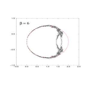
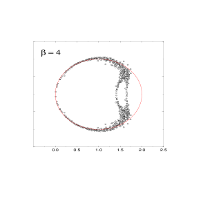
Figure 2: Plots of spectra of D2 in the complex plane for quenched gauge field configurations at $\beta=6$ (left-hand side) and $\beta=4$. The circle indicates the spectrum for exact solutions of the Ginsparg-Wilson equation.

It is easy to show, that (1) together with $\gamma_{5}$-hermiticity implies that the eigenvalues of an exact solution of the Ginsparg-Wilson equation lie on a circle of radius 1 around 1 in the complex plane. We find that the physical sector of the spectrum of D2 is very close to this limiting circle, while the doubler branches deviate considerably. This is not particularly disturbing, since the doublers decouple from the physical spectrum when driving the system to the continuum limit. Most importantly, however, we find that the physical branch intersects the real axis very close to the origin, rendering essentially massless fermions. This holds for both the $\beta=6$ and the $\beta=4$ ensemble. We furthermore find, that also the fluctuations of the eigenvalues at the origin are much smaller than the fluctuations for e.g. the standard Wilson operator with a fine tuned mass term. This leads to error bars for the $\pi$-mass (compare below) which are one order of magnitude smaller than with the standard Wilson action [15].

In order to further test the chiral properties of D2 we performed a simulation of the massless 2-flavor Schwinger model with dynamical fermions. In the continuum this model can be solved explicitly and it contains an iso-triplet of massless $\pi$-particles and a massive iso-singlet $\eta$ (for the Schwinger model with flavor see e.g. [16]). When putting the model on the lattice a violation of the chiral symmetry will lead to a non-vanishing mass for the $\pi$. The smallness of $m_{\pi}$ thus is a measure for the quality of any approximation to the Ginsparg-Wilson equation. In our simulation we compute the masses and the dispersion relations for both the $\pi$ and the $\eta$.

We compare our results to the numerical results for the two known exact solutions of the Ginsparg-Wilson equation, i.e. the overlap Dirac operator and the perfect action. The data for these cases were taken from [9]. Furthermore we compare our results also to the results for an alternative approximate solution of the Ginsparg-Wilson equation presented in [17]. In particular we compare with the truncated perfect operator augmented with an additional Clover term (TP+C). We remark, that also finite size effects can contribute to $m_{\pi}$. However, we estimated these effects to be smaller than our error bars. Furthermore, all data presented in Table 2 were computed for the same lattice size ($16^{2}$) such that for our direct comparison of lattice results finite size effects are irrelevant. All data shown in Table 2 have the same statistics ($10^{4}$ measurements).

	D2	TP+C	perfect	overlap	continuum
$m_{\pi}$	0.0340(13)	0.1304(27)	0.0088(5)	0.0038(23)	0.0
$m_{\eta}$	0.334(27)	0.347(10)	0.351(10)	0.338(13)	0.325730

Table 2: $\pi$ and $\eta$ mass at $\beta=6$ for various lattice Dirac operators as well as their values in the continuum.

In Table 2 we show, for $\beta=6$, the masses for these different approaches and also give the continuum values. For the $\pi$-mass we find a value of 0.0340 which is about four times as large as the mass obtained with the perfect action and about ten times as large as the mass from overlap. These Dirac operators are on the other hand much more expensive to simulate and still give a non-vanishing $m_{\pi}$ due to cut-offs or numerical errors. When comparing to the other approximate solution, the TP+C operator, we find that we have reduced the $\pi$-mass by a factor of 4, while the cost of the numerical simulation remained the same. We do even better for the $\eta$-mass where our data provides the best approximation of the continuum result.

Let’s now compare the dispersion relations. In Fig. 3 we show the $\pi$ and $\eta$ dispersion relations of our operator D2 (filled circles) and compare it with the dispersion relations of the other lattice approaches (symbols) as well as with the continuum result (full curve).

Figure 3: Dispersion relations for $\pi$ (left-hand side) and $\eta$. The filled circles are the numerical data for our operator D2, the triangles represent the overlap operator, diamonds the perfect action and we use squares for TP+C. The symbols are connected with dashed lines to guide the eye. The full line is the continuum result.

For the $\pi$ dispersion relation we find that the our operator leads to a nice linear behavior up to $p\sim 1$. For larger values of $p$ the dispersion curve begins to deviate from the continuum value, although not as strongly as the overlap curve. Only the perfect action manages to obtain values close to the continuum result throughout. For larger momenta also the TP+C operator is relatively close to the continuum curve, however, for $p\rightarrow 0$ the violations of chirality are obvious.

For the $\eta$ the picture is similar: Only the perfect action has a perfect dispersion relation. The other actions lead to dispersion relations which for increasing momenta deviate more or less from the continuum result. Again we find that our D2 curve lies between the continuum curve and the data for the overlap operator.

Summary In this letter we have explored a new approach to Ginsparg-Wilson fermions and tested the new method in 2-d. To keep the paper self consistent the construction of the Dirac operator was also given in 2-d, but the generalization to 4-d is straightforward and will be presented elsewhere [13].

The central idea is to construct an expansion of the Dirac operator in a suitable basis and to rewrite the Ginsparg-Wilson equation to a system of coupled quadratic equations for the coefficients. The basis elements are realized by diagrams of paths on the lattice, with the paths constituting a diagram being related by symmetries (rotations, C, P and $\gamma_{5}$-hermiticity). Although the expansion in principle has to contain infinitely many terms, the method comes with a natural cutoff: Only Dirac operators where the coefficients decrease exponentially with increasing length of the paths are of interest. Thus we can work with a finite number of terms, rendering a finite system of coupled quadratic equations. The dominating equations of the system can be solved and used to construct approximate solutions of the Ginsparg-Wilson equation.

We implemented this procedure and constructed the operator D2 which in addition to the terms appearing in the standard Wilson action only requires L-shaped terms of length 2. These terms imply only a moderate increase in the cost of a numerical simulation but drastically improve the chiral properties of the action. This was established in a numerical simulation of the 2-flavor Schwinger model.

We are currently implementing the new approach in 4-d, where the construction proceeds essentially along the lines presented here. We expect that also in 4-d a considerable improvement of the chiral properties can be achieved with only a moderate increase of the cost of a numerical simulation.

Acknowledgement: The authors thank Thomas Lippert and Uwe-Jens Wiese for insightful discussions and Christian Lang for important advice and checks of our equations.

References

- [1] F. Niedermayer, Nucl. Phys. B (Proc. Suppl.) 73 (1999) 105.
- [2] H. Neuberger, Chiral fermions on the lattice, hep-lat/9909042.
- [3] M. Lüscher, Chiral gauge theories on the lattice with exact gauge invariance, hep-lat/9909150.
- [4] P.H. Ginsparg and K.G. Wilson, Phys. Rev. D25 (1982) 2649.
- [5] P. Hasenfratz, The Theoretical Background and Properties of Perfect Actions, in: Non-Perturbative Quantum Field Physics, M. Asorey and A. Dobado (Eds.), World Scientific 1998.
- [6] W. Bietenholz and U.-J. Wiese, Nucl. Phys. B464 (1996) 319; P. Hasenfratz, Nucl. Phys. B (Proc. Suppl.) 63 (1998) 53; P. Hasenfratz, Nucl. Phys. B525 (1998) 401; P. Hasenfratz, V. Laliena and F. Niedermayer, Phys. Lett. B427 (1998) 353.
- [7] C.B. Lang and T.K. Pany, Nucl. Phys. B513 (1998) 645; F. Farchioni, C.B. Lang and M. Wohlgenannt, Phys. Lett. B433 (1998) 377, F. Farchioni, I. Hip, C.B. Lang and M. Wohlgenannt, Nucl. Phys. B549 (1999) 364.
- [8] F. Farchioni and V. Laliena, Nucl. Phys. B521 (1998) 337, Phys. Rev. D58 (1998) 054501.
- [9] F. Farchioni, I. Hip and C.B. Lang, Phys. Lett. B443 (1998) 214.
- [10] H. Neuberger, Phys. Lett. B417 (1998) 141, Phys. Lett. B427 (1998) 353.
- [11] R. Narayanan and H. Neuberger, Phys. Lett. B302 (1993) 62, Nucl. Phys. B443 (1995) 305.
- [12] D.B. Kaplan, Phys. Lett. B288 (1992) 342; Y. Shamir, Nucl. Phys. B406 (1993) 90, V. Furman and Y. Shamir, Nucl. Phys. B439 (1995) 54.
- [13] C. Gattringer A new approach to Ginsparg-Wilson fermions, hep-lat/0003005; C. Gattringer, I. Hip, C.B. Lang, Work in preparation.
- [14] I. Horvath, Phys. Rev. Lett. 81 (1998) 4063, Phys. Rev. D60 (1999) 034510; W. Bietenholz, On the absence of ultralocal Ginsparg-Wilson fermions, hep-lat/9901005.
- [15] C. Gattringer, I. Hip, C.B. Lang, Phys. Lett. B466 (1999) 287.
- [16] S. Coleman, Ann. Phys. 101 (1976) 239; L.V. Belvedere, J.A. Swieca, K.D. Rothe, B. Schroer, Nucl. Phys. B153 (1979) 112; C. Gattringer, E. Seiler, Ann. Phys. 233 (1994) 97.
- [17] W. Bietenholz and I. Hip, The scaling of exact and approximate Ginsparg-Wilson Fermions, hep-lat/9902019 (to appear in Nucl. Phys. B).