Bicocca–FT–99–40

BARI–TH 370/99

IFUP–TH 67–99

UNICAL–TH 99/6

TOPOLOGY IN 2D CP^N-1 MODELS ON THE LATTICE:

A CRITICAL COMPARISON OF DIFFERENT COOLING TECHNIQUES${}^{~{}\ast}$

B. Allés${}^{a~{}\dagger}$, L. Cosmai${}^{b~{}\ddagger}$, M. D’Elia${}^{c~{}\P}$ and A. Papa${}^{d~{}\S}$

^a Dipartimento di Fisica, Università di Milano–Bicocca and

INFN–Sezione di Milano, I–20133 Milano, Italy

^b INFN–Sezione di Bari, I–70126 Bari, Italy

^c Dipartimento di Fisica, Università di Pisa and INFN–Sezione di Pisa, I–56127 Pisa, Italy

^d Dipartimento di Fisica, Università della Calabria and INFN–Gruppo collegato di Cosenza,

I–87036 Arcavacata di Rende (Cosenza), Italy

Two-dimensional CP^N-1 models are used to compare the behavior of different cooling techniques on the lattice. Cooling is one of the most frequently used tools to study on the lattice the topological properties of the vacuum of a field theory. We show that different cooling methods behave in an equivalent way. To see this we apply the cooling methods on classical instantonic configurations and on configurations of the thermal equilibrium ensemble. We also calculate the topological susceptibility by using the cooling technique.

 ^∗Partially supported by MURST and by EC TMR program ERBFMRX-CT97-0122. $\begin{array}[]{ll}{}^{\dagger}\mbox{{\it e-mail address:}}&\mbox{\tt alles@sunmite.mi.infn.it}\\ {}^{\ddagger}\mbox{{\it e-mail address:}}&\mbox{\tt cosmai@ba.infn.it}\\ {}^{\P}\mbox{{\it e-mail address:}}&\mbox{\tt delia@mailbox.difi.unipi.it}\\ {}^{\S}\mbox{{\it e-mail address:}}&\mbox{\tt papa@cs.infn.it}\end{array}$

1 Introduction

Two–dimensional (2d) CP^N-1 models [1, 2] play an important role in quantum field theory since they represent a convenient theoretical laboratory to investigate analytical and numerical methods to be eventually exported to QCD. This is believed to be possible since these models have several important properties in common with QCD, for instance asymptotic freedom, spontaneous mass generation, confinement and topological structure of the vacuum [3]. In particular, the CP^N-1 vacuum, like the QCD one, admits instanton classical solutions. The non–trivial structure of the vacuum for the CP^N-1 models, as well as for QCD, can be probed by defining suitable operators, like the topological charge density and its correlators, and by applying the prescriptions of quantum field theory. Yet most of the observables relevant for the investigation of the vacuum topological structure of a theory are beyond the reach of perturbation theory. Therefore some approximation is needed which works also in the non–perturbative regime. So far, the most effective and comprehensive tool is represented by Monte Carlo simulations on a space–time lattice. The lattice approach for the study of the vacuum structure brings about a very delicate task, that of separating the quantum fluctuations at the level of the lattice spacing from the relevant long–distance topological ones in any given configuration of the thermal equilibrium ensemble. Indeed, trying to assign a topological charge to a thermal equilibrium configuration, treating on the same footing short–distance (quantum) fluctuations and long–distance (topological) ones, would even prevent the reaching of the continuum limit. One powerful technique, frequently adopted in the literature to study the topological structure of the vacuum, is the so–called cooling method [4]. The idea behind the cooling method is that the quantum fluctuations at the level of the lattice spacing of a given configuration can be smoothed out by a sequence of local minimizations of the lattice action, thus leading to a configuration where only the long–distance, topologically relevant fluctuations survive. When this procedure is performed on a set of well–decorrelated equilibrium configurations, it yields a “cooled” equilibrium ensemble on which the expectation values of topological quantities can be determined. The precise definition of a cooling procedure is however arbitrary to a large extent: the lattice action to be locally minimized can be chosen differently from the one used in the thermalization, the number of cooling steps is a free variable, driving or control parameters of the cooling can be introduced, and so on. Comparing the behavior of different cooling methods is an interesting issue, especially when a new cooling strategy is proposed.

The aim of the present work is to get insight into a new cooling method first adopted in Ref. [5] for the SU(2) gauge theory and to compare it with two other methods, already known in the literature, namely the “standard” [4] cooling and its controlled version adopted by the Pisa group (see for instance Ref. [6]). The new cooling method, as it will be pointed out in the next Section, follows a different strategy with respect to the other two and could possess various interesting features, inaccessible to the other two cooling methods, like for instance preserving instanton–anti-instanton (I–A) pairs with interaction energy smaller than a fixable value [5]. The test–field for this comparison will be provided by the CP^N-1 models, which have all the interesting topological properties of the SU($N$) gauge theories, but are much easier to simulate on a lattice.

The paper is organized as follows: in Section 2 we introduce the lattice action and the lattice discretization of the relevant topological quantities. In Section 3 we describe in detail the three cooling methods. In Sections 4 and 5 we discuss their performance on 1–instanton and I–A classical lattice configurations respectively. In Section 6 we consider their behavior on thermal equilibrium configurations and find a correspondence between the three cooling techniques. In Section 7 we determine the physical value of the topological susceptibility of CP⁹ using the new cooling method and compare the results to those from an alternative approach not based on cooling. Finally in Section 8 we draw our conclusions.

2 Lattice definition of action and observables

The CP^N-1 models describe the physics of a gauge invariant theory of interacting classical spins. The continuum action for the 2d CP^N-1 model is

$$S=\frac{1}{g}\int d^{2}x\,\overline{D_{\mu}z}\cdot D_{\mu}z\;,\;\;\;\;\;D_{\mu}=\partial_{\mu}+iA_{\mu}\;,$$ (1)

where $g$ is the coupling constant and $z(x)$ is a $N-$component complex scalar field which obeys the constraint $\bar{z}(x)\cdot z(x)=1$. The bar over a complex quantity means complex conjugate and a central dot among vectors implies the scalar product: $\bar{z}(x)\cdot z(x)\equiv\sum_{i=1}^{N}\bar{z}_{i}(x)z_{i}(x)$.

We regularize the theory on a square lattice using the standard discretization:

$$S^{L}=-N\beta\sum_{x}\sum_{\mu=1,2}\biggl{(}\bar{z}(x+\widehat{\mu})\cdot z(x)\,\lambda_{\mu}(x)+\bar{z}(x)\cdot z(x+\widehat{\mu})\,\bar{\lambda}_{\mu}(x)-2\biggr{)}\;,$$ (2)

where $x$ indicates a generic site of the lattice; $\lambda_{\mu}(x)$ is a U(1) gauge field ($\bar{\lambda}_{\mu}(x)\,\lambda_{\mu}(x)=1$) and $\beta\equiv 1/(Ng)$ where $g$ is the bare lattice coupling constant. We used the standard action both to generate thermal equilibrium configurations in Monte Carlo simulations and during the cooling procedure.

The continuum topological charge is defined as

$$Q\equiv\int d^{2}x\,q(x)\equiv\frac{i}{2\pi}\int d^{2}x\,\epsilon_{\mu\nu}\overline{D_{\mu}z}\cdot D_{\nu}z=\frac{1}{2\pi}\oint dx_{\mu}A_{\mu}\;,$$ (3)

where $\epsilon_{\mu\nu}$ is the antisymmetric tensor with $\epsilon_{12}=1$ and $q(x)$ is the topological charge density which can be written as the divergence of a topological current $K_{\mu}(x)\equiv 1/(2\pi)\epsilon_{\mu\nu}A_{\nu}$, $q(x)=\partial_{\mu}K_{\mu}(x)$ [1, 7]. The last integral in Eq. (3) is calculated on the 2d plane along the circle of infinite radius.

The topological susceptibility $\chi$ is a renormalization group invariant quantity which gives a measure of the amount of topological excitations in the vacuum. It is defined as the two–point zero–momentum correlation of the topological charge density operator $q(x)$,

$$\chi\equiv\int d^{2}x\,\langle 0|\,T\,[q(x)q(0)]\,|0\rangle\;.$$ (4)

This equation needs a prescription for the contact term coming from the product of operators at the same point. We use the prescription [8]

$$\chi=\int d^{2}x\,\partial_{\mu}\langle 0|\,T\,[K_{\mu}(x)q(0)]\,|0\rangle\;,$$ (5)

which corresponds to the physical requirement that $\chi=0$ in the sector with trivial topology (see for instance Ref. [9]).

On the lattice any discretization of the topological charge density with the correct naïve continuum limit can be used. A standard definition is

$$q^{L}(x)\!\equiv\!-{i\over 2\pi}\sum_{\mu\nu}\epsilon_{\mu\nu}{\rm Tr}\left[P(x)\Delta_{\mu}P(x)\Delta_{\nu}P(x)\right]\;,$$ (6)

with

$$\Delta_{\mu}P(x)\equiv\frac{P(x{+}\widehat{\mu})-P(x{-}\widehat{\mu})}{2}~{},\;\;\;\;\;P_{ij}(x)\equiv\bar{z}_{i}(x)z_{j}(x)\;.$$ (7)

The lattice topological susceptibility is defined as

$$\chi^{L}\equiv\biggl{\langle}\sum_{x}q^{L}(x)q^{L}(0)\biggr{\rangle}={1\over L^{2}}\left<\left(Q^{L}\right)^{2}\right>\;,$$ (8)

where $Q^{L}\equiv\sum_{x}q^{L}(x)$ and $L$ is the lattice size in lattice units. Unless otherwise stated, hereafter the brackets $\langle\cdot\rangle$ mean average over decorrelated equilibrium configurations.

In the CP^N-1 model $q(x)$ is a renormalization group invariant operator. Imposing that $q(x)$ does not renormalize in the continuum generally implies a finite multiplicative renormalization $Z$ on the lattice [10]

$$q^{L}(x)=a^{2}\,Z(\beta)\,q(x)+O(a^{4})\;,$$ (9)

$a$ being the lattice spacing.

Moreover, the lattice topological susceptibility $\chi^{L}$ in general does not meet the continuum prescription given in Eq. (5), thus leading to an additive renormalization which consists in mixings of $\chi^{L}$ with operators which have the same quantum numbers as $\chi$,

$$\chi^{L}(\beta)=a^{2}Z(\beta)^{2}\chi+M(\beta)\;,$$ (10)

where $M(\beta)$ indicates such mixings. The extraction of $\chi$ from the lattice thus requires the determination of both the multiplicative and additive renormalizations, $Z(\beta)$ and $M(\beta)$. This is a feasible task, as will be shown in Section 7, and in this way one obtains the so–called “field theoretical” determination of the topological susceptibility.

Alternatively one can use cooling to determine the topological susceptibility. This method will be described extensively in the next Section. The idea is that, by an iterative process of local minimization of the action, the quantum fluctuations at the scale of the ultraviolet cut–off, which are responsible for the renormalizations, are suppressed thus implying $Z\to 1$ and $M\to 0$ in Eq. (10) as the cooling iteration goes on, so that $a^{2}\,\chi$ can be extracted directly from the measurement of $\chi^{L}$ after cooling, as it will be shown in Section 7.

3 The cooling method

A cooling step applied on a lattice configuration consists in assigning to every field variable a new value chosen in order to locally minimize the lattice action. The iteration of this procedure converges to a configuration which should represent a solution of the Euclidean classical equations of motion. In the continuum 2d CP^N-1 models, as well as in the case of 4d SU($N$) gauge theories, there are classical solutions that belong to a definite topological charge sector, identified by an integer value of the topological charge $Q$ and by a finite action ($S=2\pi|Q|/g$ in the case of CP^N-1). The classical solutions with $Q\neq 0$ are called instantons or anti-instantons (depending on the sign of $Q$). On the lattice, owing to the artifacts introduced by the discretization of the theory, configurations with non–trivial topology can represent only approximated solutions of the lattice equations of motion. The common belief is that a moderately long cooling sequence can be able to wash out the quantum fluctuations of a given lattice configuration, so revealing the underlying metastable state with possible non–trivial topology, and that this state is the lattice counterpart of a continuum classical one. Of course, if the cooling is further protracted, the metastable state will eventually “decay” into the trivial vacuum. Stated in other words, once the quantum fluctuations have been eliminated and the topological bumps of a configuration (instantons or anti-instantons) have been revealed, if the cooling is further protracted then the isolated instantons or anti-instantons shrink, the I–A pairs annihilate and the configuration falls into the trivial vacuum of the lattice theory. In consideration of the above arguments, it is clear that a great care is needed in determining when a cooling iteration has to be stopped. Nevertheless, there is no way to prevent the loss of topological signal at lattice scales of the order of the lattice spacing, since topology at these scales cannot be distinguished from quantum fluctuations. It must be pointed out however, that any loss of topological signal due to cooling which occurs at fixed scales in lattice units becomes irrelevant in physical units as far as the coupling is tuned towards its critical value, i.e. in the continuum limit, when the lattice spacing $a$ tends to zero. This is not the case only when the instanton size distribution is singular in the short–distance regime, as in the 2d CP¹ model [11, 12].

In the case of the 2d CP^N-1 models, the cooling algorithm amounts to replacing at each lattice site $x$ the field variables $z(x)$ and $\lambda_{\mu}(x)$ by new ones $z^{\mathrm{new}}(x)$ and $\lambda_{\mu}^{\mathrm{new}}(x)$, chosen in order to locally minimize the lattice action, while the other field variables are left unchanged. A cooling step consists in a sweep through the entire lattice volume in order to apply this local minimization sequentially at every site $x$. The terms in the action density which depend on $z(x)$ and $\lambda_{\mu}(x)$ for a given lattice site $x$ have the form

$$s_{z}=-2\beta N\>{\rm Re}\{\bar{z}(x)\cdot F_{z}(x)\}\;,\;\;\;\;F_{z}(x)\equiv\sum_{\mu=1,2}\biggl{(}z(x-\widehat{\mu})\,\lambda_{\mu}(x-\widehat{\mu})+z(x+\widehat{\mu})\,\bar{\lambda}_{\mu}(x)\biggr{)}\;,$$ (11)

and

$$s_{\lambda}=-2\beta N\>{\rm Re}\{\bar{\lambda}_{\mu}(x)\,F_{\lambda}(x,\mu)\}\;,\;\;\;\;\;\;\;\;\;\;F_{\lambda}(x,\mu)\equiv\,\bar{z}(x)\cdot z(x+\widehat{\mu})\;,$$ (12)

where $F_{z}(x)$ and $F_{\lambda}(x,\mu)$ are the respective forces. It is easy to see that the local minimum of the lattice action is obtained when the new field variables coincide with the corresponding normalized forces:

$$z^{\mathrm{new}}(x)={F_{z}(x)\over||F_{z}(x)||}\;,\;\;\;\;\;\;\;\;\;\;\lambda_{\mu}^{\mathrm{new}}(x)={F_{\lambda}(x,\mu)\over||F_{\lambda}(x,\mu)||}\;,\;\;\;\;\;\;\;\;\;\;\mu=1,2\,,$$ (13)

with $||u||\equiv\sqrt{\bar{u}\cdot u}$ for a generic complex number or $N$–component vector $u$ ($z(x)$, $F_{z}(x)$, $\lambda_{\mu}(x)$, $F_{\lambda}(x,\mu)$, etc.). According to the supplementary conditions under which the above replacements are performed, we have different cooling procedures. The first cooling procedure, which we call “standard”, is the one where the replacements $z(x)\rightarrow z^{\mathrm{new}}(x)$ and $\lambda_{\mu}(x)\rightarrow\lambda_{\mu}^{\mathrm{new}}(x)$ are unconstrained. The second one, which we call “Pisa cooling”, is the one where the replacement of $z(x)$ and $\lambda_{\mu}(x)$ is performed if the distance between the old and the new fields is smaller than a previously fixed parameter $\delta_{\rm Pisa}$: $||\lambda_{\mu}(x)-\lambda_{\mu}^{\mathrm{new}}(x)||\leq\delta_{\rm Pisa}$ and analogously for the $z$ fields, otherwise the new field is chosen to lie on the $(z(x),z^{\mathrm{new}}(x))$ ($(\lambda_{\mu}(x),\lambda_{\mu}^{\mathrm{new}}(x))$) plane, at a distance from $z(x)$ ($\lambda_{\mu}(x)$) exactly equal to $\delta_{\rm Pisa}$ [6]. The third cooling procedure, called “new cooling” in the following, was introduced in Ref. [5]. It consists in making the replacement only if the distance between the old and new fields is larger than a fixed parameter $\delta$, otherwise the field is left unchanged. We observe that the three methods follow a different strategy. In particular, while the Pisa cooling acts first on the smoother fluctuations and the number of cooling iterations to be performed has to be fixed a priori, the new cooling performs local minimizations only if these fluctuations are larger than a given threshold and the iteration stops automatically when all the surviving fluctuations are smoother than the (lattice) threshold determined by the dimensionless parameter $\delta$. It is easy to see that the new field variables differ from the old ones by terms which, in the continuum limit, are of order $a^{2}$, where $a$ is the lattice spacing. Therefore the parameter $\delta$ is expected to scale in the continuum limit like a quantity of dimension two.

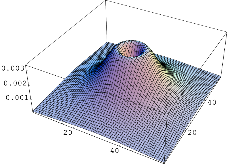
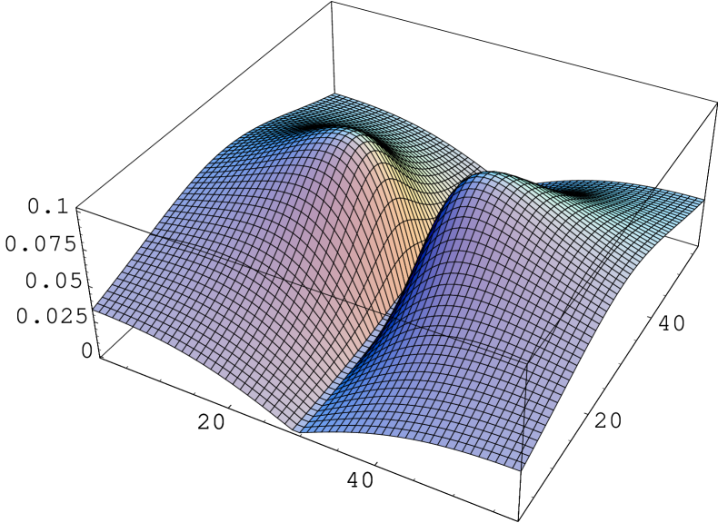
Figure 1: $\theta_{z}(x)$ (left) and $\theta_{\lambda}(x,1)$ (right) for an “artificial” 1–instanton with size $\rho=10a$ placed in the middle of a $60^{2}$ lattice.

In the following we will compare these three cooling methods in several contexts, namely on “artificial” 1–instanton configurations, on I–A pairs, on thermal equilibrium configurations and in the determination of the continuum topological susceptibility. Moreover we will establish a relation between the number of cooling iterations in the standard and Pisa coolings with the parameter $\delta$ of the new cooling and will discuss the validity of the picture of cooling as a diffusion process.

4 Cooling 1–instanton configurations

In the continuum CP^N-1 models, in the infinite 2d space–time, a 1–instanton configuration is a classical solution of the equations of motion characterized by a topological charge one and a finite action ($S=2\pi/g$). The explicit form of a continuum 1–instanton configuration is

$$z(x)=\frac{w(x)}{||w(x)||}\;,\;\;\;\;\;A_{\mu}=i\bar{z}(x)\cdot\partial_{\mu}z(x)\;,$$ (14)

with

$$w(x)=u+\frac{(x_{1}-c_{1})-i(x_{2}-c_{2})}{\rho}\,v\;,$$ (15)

where $u$ and $v$ are complex $N$–vectors which satisfy $\bar{u}\cdot u=\bar{v}\cdot v=1$ and $\bar{u}\cdot v=0$. The space–time coordinates $(c_{1},c_{2})$ are the center of the instanton and the real parameter $\rho$ represents a measure of its size. An “artificial” 1–instanton lattice configuration can be represented by the discretization of the above continuum configuration on a 2d finite volume lattice with periodic boundary conditions. In particular, we used the following expressions for the fields $z$ and $\lambda$ [1]

$$z_{1}(x)=\frac{\rho}{\sqrt{\rho^{2}+(x_{1}-c_{1})^{2}+(x_{2}-c_{2})^{2}}}\;,\;\;\;z_{2}(x)=\frac{x_{1}-c_{1}-i(x_{2}-c_{2})}{\sqrt{\rho^{2}+(x_{1}-c_{1})^{2}+(x_{2}-c_{2})^{2}}}\;,$$

$$z_{i}(x) = 0\;,\;\;\;\;\;i=3,\ldots,N\;,$$

$$\lambda_{\mu}(x) = \frac{\bar{z}(x+\widehat{\mu})\cdot z(x)}{||\bar{z}(x+\widehat{\mu})\cdot z(x)||}\;,$$ (16)

which correspond to choose $u=(1,0,0,\dots)$ and $v=(0,1,0,0,\dots)$. Actually 1–instanton configurations cannot exist on a 2d torus even in the continuum [13] and they represent only approximate solutions of the classical equations of motion. This approximation becomes better and better as the ratio $\rho/(La)$ decreases. On the lattice, this problem would lead to metastability even in the case of an ideally perfect discretization. However the above–defined artificial 1–instanton lattice configurations are enough for our purposes since they will be used only as test configurations for cooling methods and not to extract physical information.

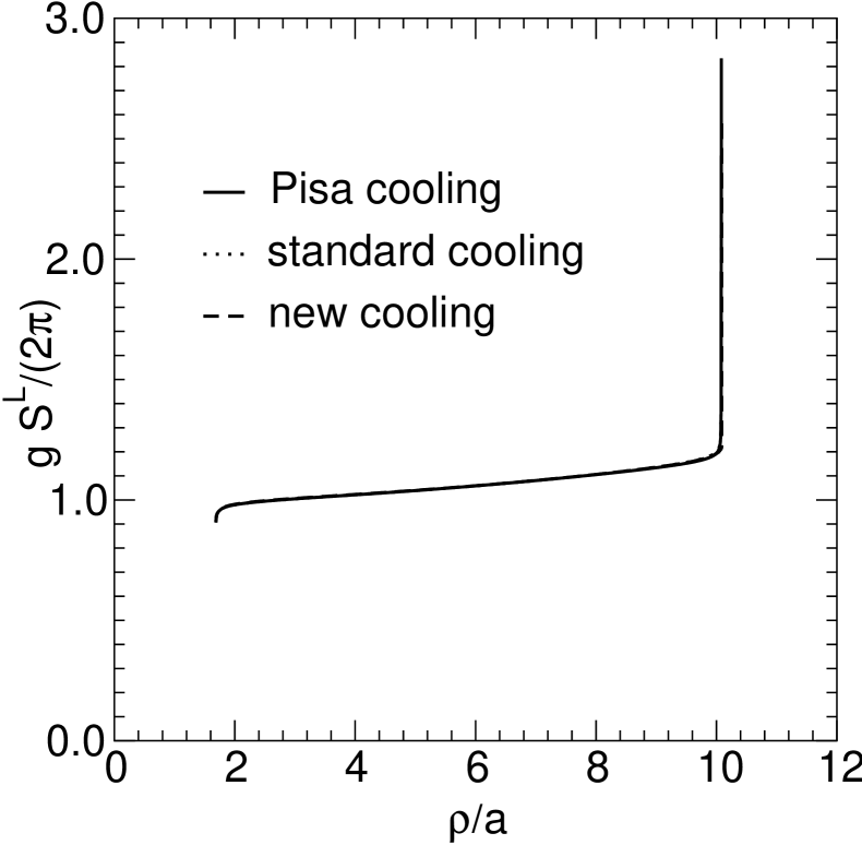
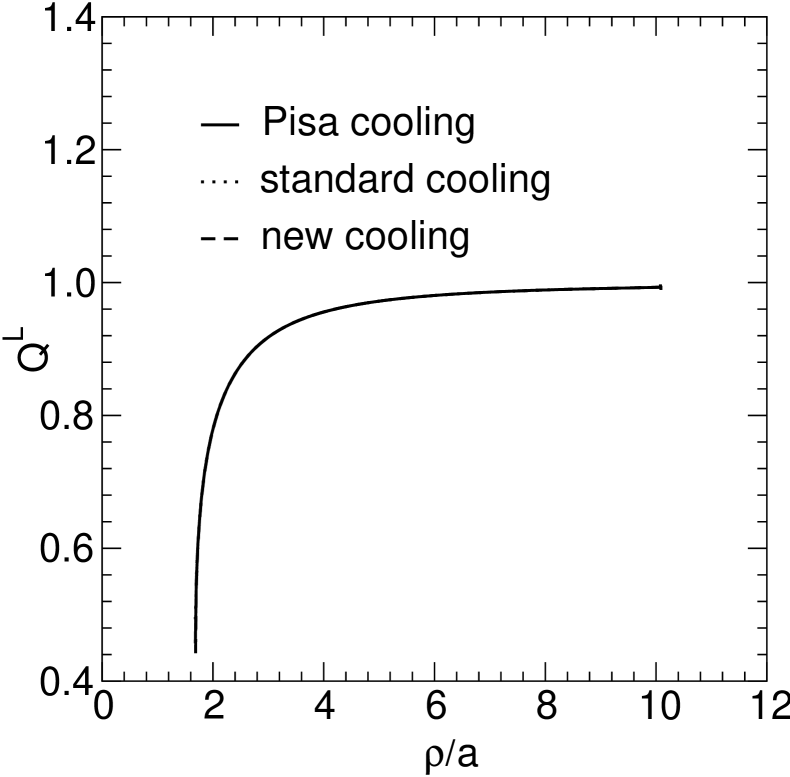
Figure 2: $g\,S^{L}/(2\pi)$ (left) and $Q^{L}$ (right) versus $\rho/a$ during a protracted cooling iteration with the three cooling methods. The starting configuration is a 1–instanton with size $\rho=10a$ placed in the middle of a $60^{2}$ lattice.

In Fig. 1 we show the distribution of the angles $\theta_{z}(x)$ and $\theta_{\lambda}(x,1)$ for an artificial 1–instanton with size $\rho=10a$ located in the middle of a $60^{2}$ lattice. These angles are defined as

$$||\lambda_{\mu}(x)-\lambda_{\mu}^{\rm new}(x)||\equiv 2\sin{\theta_{\lambda}(x,\mu)\over 2}\;,\qquad\qquad\qquad||z(x)-z^{\rm new}(x)||\equiv 2\sin{\theta_{z}(x)\over 2}\,.$$ (17)

It is clear that, while the standard cooling acts indistinctly on each lattice site, the Pisa cooling and the new cooling deform 1–instanton lattice configurations starting from different regions of the lattice. The new cooling will act first on the region around the center of the instanton, the Pisa cooling on the border regions. Therefore it is not obvious whether under the three coolings the configurations will look the same sweep after sweep. We did therefore the following check: we performed a long ($O(1000)$ steps) iteration of the standard and Pisa coolings on an artificial 1–instanton configuration with size $\rho=10a$ and after each sweep we extracted the topological charge $Q^{L}$, the action $S^{L}$ and the size $\rho/a$. This size was determined by a very local procedure, namely by looking for the maximum of the lattice action density $s^{L}_{\mathrm{max}}$ and using the relation $s^{L}_{\mathrm{max}}=2a^{2}/\rho^{2}$, valid for a 1–instanton configuration. Then, starting from the same configuration, we applied the new cooling for $\delta$ as small as $5\times 10^{-4}$ and for each configuration obtained during the cooling iteration, we determined again $Q^{L}$, $S^{L}$ and $\rho/a$. Finally, we put on a plot $Q^{L}$ and $S^{L}$ as functions of $\rho/a$. The result is shown in Fig. 2: the values of $Q^{L}$ and $S^{L}$ during the three cooling methods lie on the same curve. The same plot was obtained by using a different procedure to determine the size of the cooled configurations, namely a global fit of the lattice action density to the continuum expression for the action density of a 1–instanton configuration, Eq. (14). We interpret these results as an indication that the three coolings deformed in the same way the starting configuration. If this conjecture is correct, it should be possible to put into correspondence the $\delta$ parameter of the new cooling with the number of steps of the standard or Pisa coolings. This will be done in Section 6.

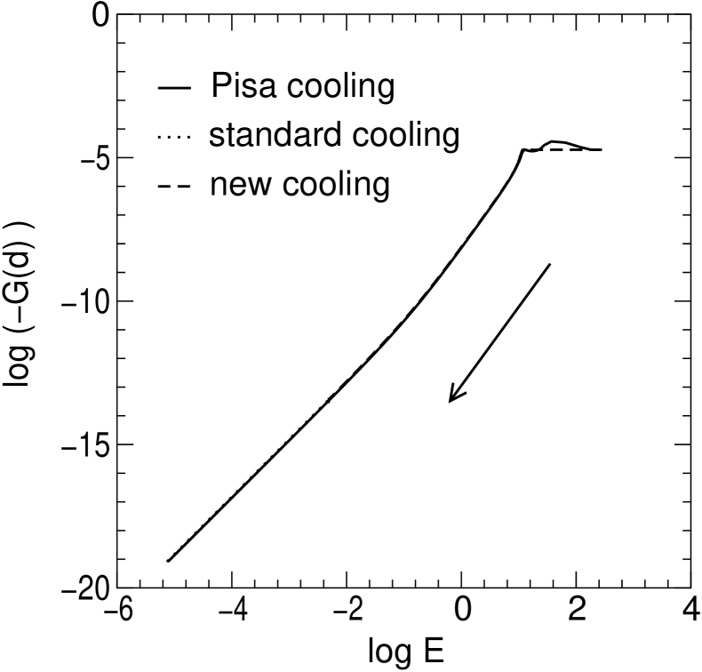
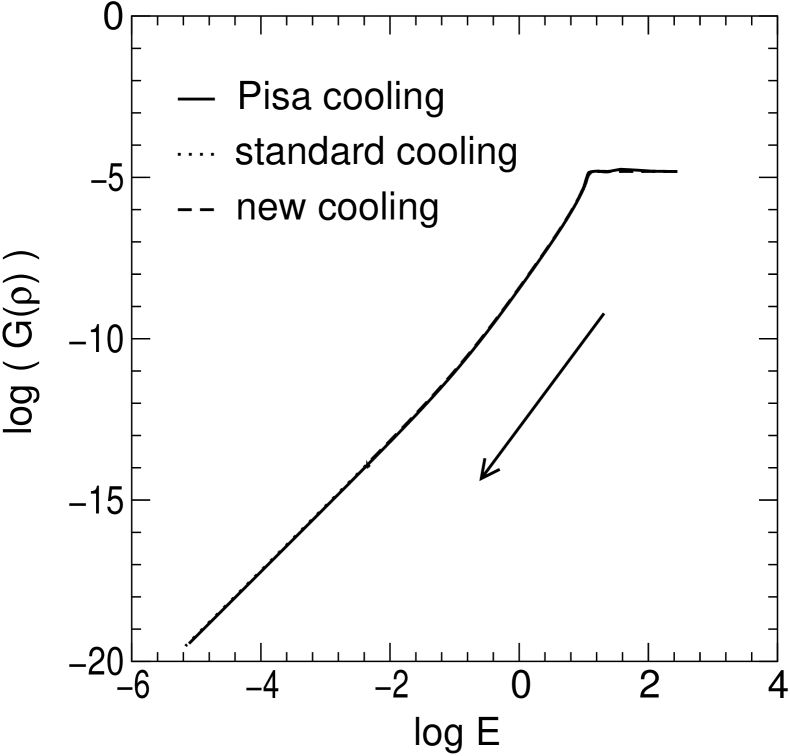
Figure 3: ${G}(d)$ (left) and ${G}(\rho)$ (right) versus the internal energy $E$ during a protracted cooling iteration with the three cooling methods in a log–log scale. The starting configuration is an I–A pair with centers $c^{(I)}=(15a,30a)$, $c^{(A)}=(45a,30a)$ (hence $d\equiv|c^{(I)}-c^{(A)}|=30a$) and $\rho=5a$ on a $60^{2}$ lattice. The arrows show the direction of the evolution under cooling.

5 Cooling I–A pairs

An I–A configuration in the continuum 2d CP^N-1 models can be taken in the form given in Refs. [15, 16],

$$z(x)=\frac{w(x)}{||w(x)||}\;,\;\;\;\;\;A_{\mu}=i\bar{z}(x)\cdot\partial_{\mu}z(x)\;,$$ (18)

with

$$w_{1}(x_{1},x_{2}) = (x_{1}+ix_{2}-a_{1})(x_{1}-ix_{2}-\bar{b}_{1})\;,$$

$$w_{2}(x_{1},x_{2}) = (x_{1}+ix_{2}-a_{2})(x_{1}-ix_{2}-\bar{b}_{2})\;,$$

$$w_{i} = 0\;,\;\;\;\;\;i=3,\ldots,N\;.$$ (19)

In this expression, the complex numbers $a_{1,2}$ and $b_{1,2}$ are related to the position of the center and the size of the instanton and anti-instanton through the following relations:

$$a_{1}=c^{(I)}_{1}+ic^{(I)}_{2}-\rho^{(I)}\;,\;\;\;\;\;\;\;\;\;\;a_{2}=c^{(I)}_{1}+ic^{(I)}_{2}+\rho^{(I)}\;,\;\;\;\;\;\;\;\;\;\;$$

$$b_{1}=c^{(A)}_{1}+ic^{(A)}_{2}-\rho^{(A)}\;,\;\;\;\;\;\;\;\;\;\;b_{2}=c^{(A)}_{1}+ic^{(A)}_{2}+\rho^{(A)}\;,\;\;\;\;\;\;\;\;\;\;$$ (20)

where $c_{i}^{(I,A)}$ is the $i$–th coordinate of the center of the instanton or anti-instanton and $\rho^{(I,A)}$ are their sizes. As “artificial” I–A lattice configuration we took the discretization of the above continuum configuration on a 2d finite volume lattice with periodic boundary conditions. For simplicity, we used $\rho^{(I)}=\rho^{(A)}\equiv\rho$.

Starting from several I–A pairs with different values of the distance between the centers $c^{(I)}$ and $c^{(A)}$ and of the size $\rho$, we performed long cooling sequences with the three methods, namely $O(1000)$ iterations for the standard and Pisa coolings and $\delta$ as small as $5\times 10^{-4}$ for the new cooling. In order to have an indication of how the cooling process works, we examined by eye the distribution of the topological charge and action densities during the different cooling iterations. The evolution of these densities looked the same, no matter which cooling procedure was adopted. Specifically, the distribution of the action density shows at the beginning two equal instanton bumps, which for $d\gg\rho$ ($d$ is the distance between the two centers $c^{(I)}$ and $c^{(A)}$) are well–separated; then, as the cooling goes on, these bumps lower in height and merge together, up to complete annihilation. In order to make quantitative the statement that the three coolings behave essentially in the same way, we studied the shell correlation function of the topological charge density. This function is defined as ${G}(r)\equiv 1/N_{r}\sum_{x,y}q^{L}(x)q^{L}(y)$ where the sum is extended over all pairs of sites $x$, $y$ which satisfy $r\leq|x-y|<r+\Delta\,r$ and $N_{r}$ is the number of those pairs for a given value of $r$ (we have chosen $\Delta\,r=0.6\,a$). We determined ${G}(r)$ on every configuration resulting after each cooling iteration. We compared the results which presented the same value for the internal energy $E$ which is defined by

$$E\equiv\frac{1}{2L^{2}}\,\sum_{x}\sum_{\mu=1,2}\left(\bar{z}(x+\widehat{\mu})\cdot z(x)\,\lambda_{\mu}(x)+\bar{z}(x)\cdot z(x+\widehat{\mu})\,\bar{\lambda}_{\mu}(x)-2\right)\;,$$ (21)

and is proportional to the lattice action. In Fig. 3 we show the behavior of the shell correlation versus $E$ during the three (protracted) coolings for the case of $r$ equal to the distance $d$ between the centers of the instanton and of the anti-instanton (left) and to the instanton (or anti-instanton) size $\rho$ (right). The three curves fall on top of each other, apart from a small deviation between the Pisa cooling and the other two at the very first (1–2) cooling steps, due to (unphysical) finite size effects. Since the shell correlation of the topological charge density is related to the size of the instantons, the conclusion is that the three cooling methods perform equivalently in deforming the size of both the instanton and the anti-instanton in the I–A pair and in modifying the distance between the two peaks.

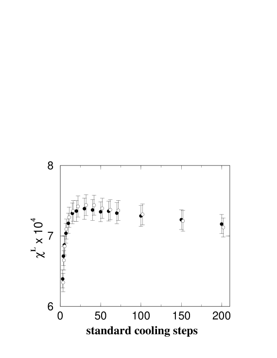
Figure 4: Comparison of the determinations of $\chi^{L}$ after equivalent amounts of new and standard coolings for the CP³ model at $\beta=1.05$ on a $76^{2}$ lattice. The new cooling results are reported versus equivalent iterations of standard cooling steps following Table 1. Full (open) symbols indicate the new (standard) cooling.

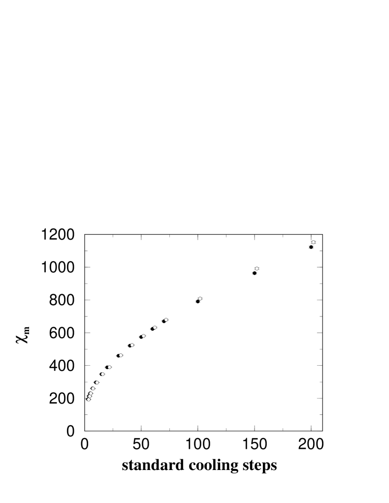
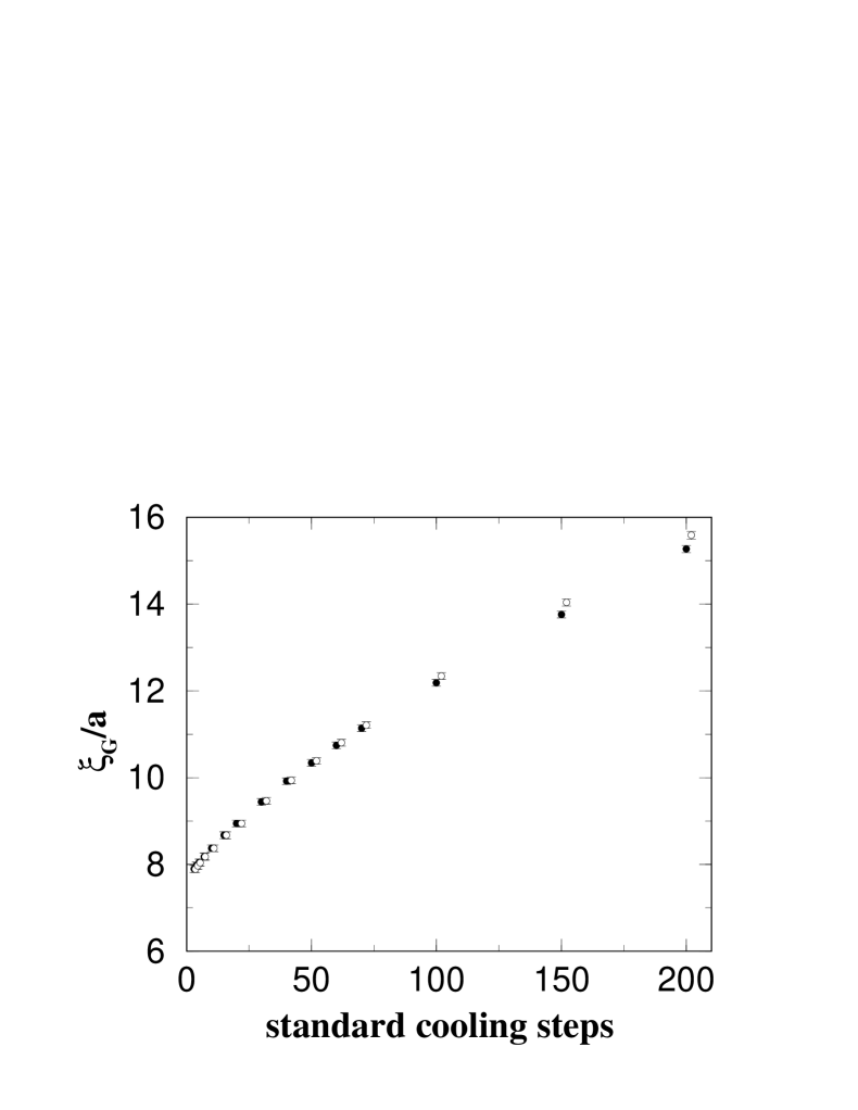
Figure 5: The same comparison as in Fig. 4 for the magnetic susceptibility and the correlation length as defined in Eq. (22). Data points have been horizontally shifted for the sake of readability. Full (open) symbols indicate the new (standard) cooling.

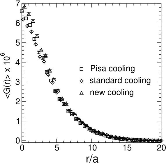
Figure 6: Two–point shell correlation of the lattice topological charge density operator ($r$ is the distance between two lattice sites) after cooling for the CP³ model at $\beta=1.05$ on a $76^{2}$ lattice. The data have been slightly horizontally shifted.

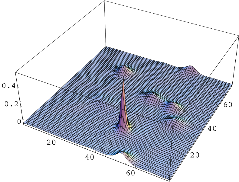
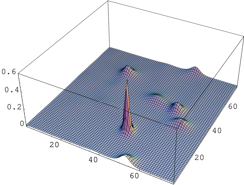
Figure 7: Action density for a configuration obtained by cooling a thermal equilibrium configuration of CP³ at $\beta=1.05$ on a $76^{2}$ lattice by the new cooling with $\delta=0.007$ (left) and by 30 iterations of the standard cooling (right). The two amounts of cooling are equivalent in the sense explained in the text.

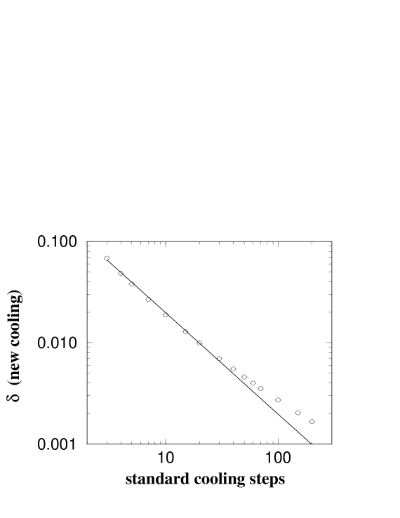
Figure 8: Relation between the new cooling parameter $\delta$ and the number of standard cooling iterations $n$, at $\beta=1.05$ on a lattice $76^{2}$ in the CP³ model, together with a best fit to a function proportional to $1/n$.

6 Cooling on the equilibrium ensemble

Using artificial configurations with non–trivial topology provides interesting suggestions about a cooling procedure, but in real life the cooling must be applied on thermal equilibrium configurations. Among them there are configurations which contain several instanton and anti-instanton bumps, merged in a sea of quantum fluctuations. These configurations can represent as well good test–fields for the different cooling procedures. Their evolution under cooling can be visualized by the distribution of the action density or of the topological charge density. In principle we could expect that the three cooling methods described in Section 3 make the starting thermalized configuration evolve along different directions. In particular, for a not too protracted cooling, one expects that all the three methods have been able to erase the quantum fluctuations, but the number, type and location of the surviving topological bumps in the cooled configuration can be rather different. In order to check this expectation, it is necessary to find a criterion to make a correspondence between the number of iterations in the standard or Pisa coolings with a $\delta$ parameter for the new cooling. We defined an effective temperature for configurations obtained during the cooling iteration in such a way that the comparison could be made only between configurations at the same temperature. The most natural “thermometer” is the internal energy $E$, Eq. (21), since this is the quantity which is minimized during the cooling procedure.

We put into practice the above considerations in the case of the CP³ model. We generated by Monte Carlo a sample of equilibrium configurations on a $76^{2}$ lattice at $\beta=1.05$. As in Ref. [14], the simulation algorithm is, for every updating step, a mixture of 4 microcanonical updates and 1 over heat–bath [17]. We measured the expectation value of $E$ on the cooled ensembles obtained by the three cooling methods after several number of iterations (standard and Pisa coolings) and for several values of $\delta$ (new cooling). By comparing the results and imposing that $E$ be the same, we obtained a correspondence table between the number of cooling iterations for the standard and Pisa coolings with a value of the $\delta$ parameter in the new cooling. We found for instance that for the CP³ model at the above values of $\beta$ and lattice size, 30 iterations of the standard cooling correspond (in the sense of the average value of $E$) to $\delta=0.007$ for the new cooling and to approximately 33 iterations of the Pisa cooling.

In general the matching between the number of standard and Pisa cooling iterations is not as good as the one obtained between $\delta$ in the new cooling and a fixed number of iterations in the standard (or Pisa) cooling. The reason is that in the second case one can tune a continuous parameter while in the first only integer jumps of the parameter controlling the amount of cooling are allowed. For this reason we have mainly investigated the relation existing between the standard and new coolings. In Table 1 we show the values of $\delta$ (new cooling) found in correspondence to several numbers of iterations of the standard cooling for the CP³ model at $\beta=1.05$ on a $76^{2}$ lattice. Notice that a different correspondence table may be found for other values of $N$ and $\beta$.

Using the correspondence table we can directly compare the different coolings. As a first step, we have computed the average values of some physical quantities on samples obtained after applying equivalent amounts of cooling on a set of equilibrium configurations. In Fig. 4 we show the results for the lattice topological susceptibility with the standard and new coolings. By using the relation given in Table 1, we report both determinations in terms of the number of standard cooling iterations. It clearly appears that, regarding to the determination of the topological susceptibility, the two cooling techniques are completely equivalent.

Analogously in Fig. 5 we compare the determinations of the magnetic susceptibility $\chi_{\rm m}$ and of the correlation length $\xi_{G}$ defined by

$$\chi_{\rm m} \equiv {1\over L^{2}}\sum_{x,y}\langle\hbox{Tr}P(x)P(y)\rangle_{\rm conn}\;,$$

$$\left(\frac{\xi_{G}}{a}\right)^{2} \equiv {1\over 4\sin^{2}(\pi/L)}\,\left[\frac{\widetilde{G}_{P}(0,0)}{\widetilde{G}_{P}(0,1)}-1\right]\;,$$ (22)

where

$$\widetilde{G}_{P}(k)\equiv\frac{1}{L^{2}}\sum_{x,y}\langle{\rm Tr}\>P(x)\,P(y)\rangle_{\rm conn}\exp\left[i\frac{2\pi}{L}(x-y)\cdot k\right]\,,$$ (23)

is the lattice Fourier transform of the correlation of two local gauge–invariant composite operators $P_{ij}(x)$ which have been defined in Eq. (7) (the subscript “conn” means connected Green function). The results for $\chi_{\rm m}$ and $\xi_{G}/a$ from Fig. 5 indicate that in this case the new cooling and the standard cooling show a good agreement, apart from a small discrepancy at large numbers of iterations.

We have also studied the shell correlation of two lattice topological charge density operators, $\langle{G}(r)\rangle$, for $r/a$ going from 0 to 20, after equivalent amounts of the three coolings. In Fig. 6 we compare the standard cooling (30 iterations) to the new cooling ($\delta=0.007$) and the Pisa cooling (33 iterations, $\delta_{\rm Pisa}=0.2$). The results are in good agreement, although a small deviation can be observed at small distances. The suggestion of this outcome is that the three coolings affect the instanton size distribution in the small distance region in a slightly different way; the effect is however modest.

Next we compared the three coolings on a subset of the above–generated thermal equilibrium ensemble for the CP³ model. To this aim, we have chosen from the thermal ensemble several configurations showing non–zero topological charge after 30 iterations of the standard cooling and compared their action density and topological charge density distributions by eye to those of the same configurations cooled by 33 iterations of the Pisa cooling and by the new cooling with $\delta=0.007$. For all the configurations considered, we observed that the bumps corresponding to instantons and anti-instantons had the same shape, number and location (see Fig. 7 for an example).

These considerations provide evidence that the three cooling methods defined in Section 3 behave essentially in an equivalent way, not only on average, but also configuration by configuration, and that they can be related by a simple correspondence between number of iterations (standard and Pisa coolings) and $\delta$ (new cooling).

We close this Section with some considerations about the usual picture of cooling as a diffusion process. As we pointed out in Section 3, the parameter $\delta$ in the new cooling behaves, in the continuum limit, like a physical quantity of dimension two. Therefore, indicating with $r_{0}$ the physical scale up to which cooling affects the quantum fluctuations and following Ref. [5], we infer that $r_{0}\propto\delta^{-1/2}$ in the continuum limit. On the other hand, the standard cooling is usually believed to act as a diffusion process, so that, if $n$ is the number of iterations, it should affect fluctuations up to a scale $r_{0}\propto n^{1/2}$. Using the relation found between $n$ and $\delta$, we can check both these predictions: indeed we expect that $\delta\propto 1/n$. In Fig. 8 we have plotted the function $\delta(n)$ given in Table 1, together with a best fit to a function proportional to $1/n$. For the lattice parameters used in the simulation we see that $\delta(n)$ behaves as expected for small values of $n$, while the relation $\delta\propto 1/n$ breaks down for $n\gtrsim 30-40$, indicating that the picture of the standard cooling as a diffusion process may work well only for moderately small values of $n$.

7 The topological susceptibility

In this Section we apply the new cooling method to the determination of the physical topological susceptibility and compare the results to those from an alternative approach, the field theoretical method [18] combined with smearing [19]. As for the comparison of the new cooling with the standard and Pisa coolings, we have already shown in the previous Section that they give equivalent results for $\chi^{L}$.

The lattice discretization of the topological charge density and of the topological susceptibility has already been discussed in Section 2. In the relation existing between the lattice topological susceptibility $\chi^{L}$ and the continuum one, Eq. (10), $M(\beta)$ indicates the mixings of $\chi^{L}$ to operators with the same quantum numbers. More precisely one can write

$$M(\beta)=A(\beta)\,a^{2}\langle T\rangle_{\rm np}+P(\beta)\langle I\rangle+O(a^{4})\;.$$ (24)

The first and second terms in the r.h.s. are the mixings with the trace of the energy–momentum tensor and with the unit operator respectively (“np” means the purely non–perturbative part of $\langle T\rangle$).

The mixing coefficients $A(\beta)$ and $P(\beta)$ as well as the multiplicative renormalization $Z(\beta)$ can be calculated in perturbation theory. The perturbative series for $A(\beta)$ starts from the order $1/\beta^{3}$ and arguments can be given [11] which justify that $A(\beta)\,a^{2}\langle T\rangle_{\rm np}$ is safely negligible in the scaling window of the simulation. In Ref. [20] the perturbative series for $Z(\beta)$ has been calculated up to the order $1/\beta^{2}$ and the perturbative series of $P(\beta)$ at the first two non–zero orders $1/\beta^{4}$ and $1/\beta^{5}$. On the other hand there are no available perturbative estimates of the $O(a^{4})$ terms in Eq.(24).

However, a more powerful, purely numerical technique can be used to get a non–perturbative determination of $Z(\beta)$ and of the whole additive renormalization $M(\beta)$. This technique is the so–called “heating method” [21].

The idea of the heating method is to determine the average values of topological quantities on samples of configurations obtained by thermalizing the short–range fluctuations, which are responsible for the renormalizations, on configurations of well defined topological background. For instance if one applies several thermalization steps at a given value of $\beta$ on a configuration containing one discretized instanton of charge $Q=1$ and measures the average value of $Q^{L}$, then the renormalization constant $Z(\beta)$ can be determined as $Z(\beta)=\langle Q^{L}\rangle/Q$ (here $\langle\cdot\rangle$ indicates an average in the background of a fixed charge $Q$). Analogously, by thermalizing a trivial configuration (for example a configuration where for all lattice sites $x$, the respective fields are $z(x)=(1,0,0,\dots)$ and $\lambda_{\mu}(x)=1$) at a given $\beta$ and measuring the average value of $\chi^{L}$, one gets a determination of $M(\beta)$. In the first case one obtains a non–perturbative estimate of $Z(\beta)$ as long as the $\overline{\hbox{MS}}$ value of the background topological charge $Q$ is chosen (see Section 2). In the second case the method amounts to impose the requirement that the physical susceptibility $\chi$ vanishes in the absence of instantons.

The heating method has been extensively applied in the following. Once all the renormalization constants are known, the extraction of $\chi$ from Eq. (10) is possible and the result is called the field theoretical determination.

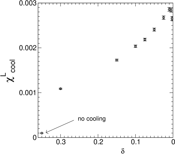
Figure 9: $\chi^{L}_{\mathrm{cool}}$ as a function of the $\delta$ parameter of the new cooling for CP⁹ at $\beta=0.70$ on a $24^{2}$ lattice.

Since the continuum $\chi$ is extracted from the lattice $\chi^{L}$ by subtracting the renormalization effects, it happens that, if $M(\beta)$ is a large part of the whole lattice signal and $Z(\beta)$ is small, the physical signal for $\chi$ is extracted with very large errors. This is the case when one uses the lattice discretization of Eq. (6). However, since both $Z(\beta)$ and $M(\beta)$ depend on the discretization $q^{L}(x)$, one can exploit the arbitrariness in the lattice definition and use an improved operator. To this aim, following the idea of Ref. [19], already used for the determination of $\chi$ in Yang–Mills theories [22], we have used a smeared topological charge density operator, which is built from the original operator $q^{L}(x)$, defined in Eq. (6), by replacing the fields $z(x)$ and $\lambda_{\mu}(x)$ with

$$z^{\mathrm{smear}}(x)={\mathcal{N}}_{z}\biggl{[}(1-c)z(x)+\frac{c}{4}\sum_{\mu=1,2}\biggl{(}z(x-\widehat{\mu})\,\lambda_{\mu}(x-\widehat{\mu})+z(x+\widehat{\mu})\,\bar{\lambda}_{\mu}(x)\biggr{)}\biggr{]}\;,\;\;\;\;$$

$$\lambda_{\mu}^{\mathrm{smear}}(x)={\mathcal{N}_{\lambda}}\biggl{[}(1-c)\lambda_{\mu}(x)+c\,\frac{\bar{z}(x)\cdot z(x+\widehat{\mu})}{||\bar{z}(x)\cdot z(x+\widehat{\mu})||}\biggr{]}\,,$$ (25)

where ${\mathcal{N}}_{z}$, ${\mathcal{N}_{\lambda}}$ are normalization constants which allow that $||z^{\rm smear}(x)||=||\lambda_{\mu}^{\rm smear}(x)||=1$ and $c$ has been chosen to be equal to 0.65 . The smearing can be iterated at will by defining the $n$–th level of smeared fields from the $(n-1)$–th level in an analogous fashion as shown in Eq. (25). For each level of smearing a relation like Eq. (10) holds although $Z(\beta)$ and $M(\beta)$ change. Using smeared operators these renormalization constants get closer to 1 and 0, respectively, as the smearing level increases, thus allowing a much more precise determination of $\chi$.

We performed a numerical simulation for the CP⁹ model at several values of $\beta$ and $L$. We used the same updating algorithm of the previous Section. For most simulations we collected 100K equilibrium configurations after discarding 10K configurations to allow thermalization. The successive equilibrium configurations were decorrelated by 10 updating steps. By averaging on the thermal equilibrium ensemble we determined the unsmeared lattice topological susceptibility $\chi^{L}$ and the smeared ones, $\chi^{L}_{\mathrm{smear}}$, for 1 to 10 smearing levels. These results, together with $Z(\beta)$ and $M(\beta)$ coming from the heating method, allow to extract $a^{2}\chi$ from Eq. (10).

Every 50 updating steps we have also applied the new cooling method at several values of the $\delta$ parameter ranging from 0.3 to $5\times 10^{-4}$. Since cooling eliminates the short–distance fluctuations, the value of $\chi^{L}$ after cooling, hereafter called $\chi^{L}_{\mathrm{cool}}$, can be written as in Eq. (10) with $Z\approx 1$ and $M\approx 0$ if the cooling has been protracted enough. Hence it should provide directly $a^{2}\chi$. Consistency requires that the cooling and the field theoretical methods provide the same result.

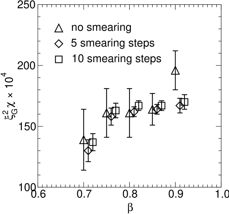
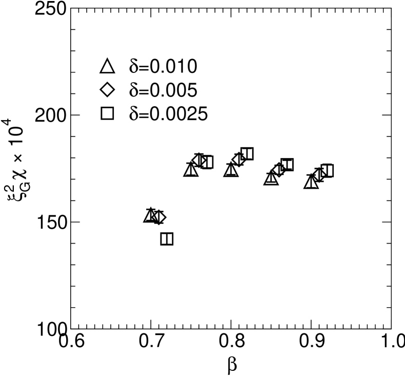
Figure 10: Scaling of the topological susceptibility of CP⁹ from the field theoretical with smearing (left) and from the new cooling (right). Data points have been slightly shifted along the $\beta$ axis for the sake of readability.

The summary of the performed simulations is presented in Table 2. In Fig. 9 we show the results for $\chi^{L}_{\rm cool}$ from the new cooling at several values for the $\delta$ parameter at $\beta=0.70$ on a $24^{2}$ lattice. We interpret the behavior under the new cooling in the following way: as $\delta$ decreases, the cooling erases an even larger amount of quantum fluctuations thus bringing $\chi^{L}_{\rm cool}$ to a maximum. Afterwards, for too small values of $\delta$, the cooling begins to affect also the topological fluctuations and part of the topological signal gets lost. These considerations suggest that a convenient choice of the $\delta$ parameter may be around the value for which $\chi^{L}_{\rm cool}$ reaches the maximum. At this value of $\delta$ we then assume that $Z\approx 1$ and $M\approx 0$. The choice of a smaller value for $\delta$ would not be dramatically dangerous, but would push the scaling region towards larger values of $\beta$.

In Table 3 we summarize the results for $\chi^{L}$ and for $\xi_{G}^{2}\,\chi$ obtained for CP⁹ by the field theoretical method combined with smearing (0, 5 and 10 levels). In Table 4 the results for $\chi^{L}_{\mathrm{cool}}$ and $\xi^{2}_{G}\,\chi$ obtained by the new cooling method for $\delta$ around the peak value (see Fig. 9 for $\beta=0.70$) are shown. Fig. 10 displays the scaling of $\xi_{G}^{2}\,\chi$ for the cases of 0, 5 and 10 smearing levels and the field theoretical method (left) and with the new cooling method for $\delta$=0.0100, 0.0050, 0.0025 (right). From this figure we see that there is practically no dependence on the smearing level, although error bars strongly decrease with the number of smearing levels. As for the cooling method, we see that there is a satisfying consistence among the results for the different values of $\delta$ and also between these results and those from the field theoretical method.

8 Summary and conclusions

The study of the topological properties of the vacuum of a field theory simulated on a lattice is made difficult by the presence of quantum fluctuations which hinder the extraction of the relevant physical information. Among other methods, cooling has been proposed as a technique to wash out such fluctuations and reveal the topological background of any single field configuration. In the present paper we have made a comparison among three different cooling methods using as test–field the 2d CP^N-1 model defined in Section 2.

The three cooling methods under study have been defined in Section 3. They are: the standard cooling (a local minimization of the Euclidean lattice action), the Pisa cooling (the same but with local minimizations constrained to be smaller than a given bound) and a new cooling (recently introduced in Ref. [5]) where the local minimizations are accepted only if they are larger than a given bound.

Firstly, we have studied the performance of the three coolings on classical non–equi-librium configurations representing 1–instanton solutions and instanton–anti-instanton pairs. We have placed one such object on the lattice and have performed a series of cooling iterations in order to measure several physical (topological and non–topological) observables. In all situations the three coolings have yielded the same result —see Figs. 2 and 3.

After these results, we have assumed that the three cooling methods are equivalent and that a correspondence can be established between them in the sense that a given number of iterations of the Pisa or the standard coolings corresponds to a precise value for the bound in the new cooling if the value of the energy $E$, Eq. (21), is the same after applying the coolings. This correspondence has been used in the subsequent investigation and, for the CP³ model at $\beta=1.05$ on a $76^{2}$ lattice, it is shown in Table 1.

We have studied the performance of the cooling methods on a set of equilibrium configurations obtained after a Monte Carlo simulation. On these thermalized configurations we have first extracted several physical quantities after applying cooling: the lattice topological susceptibility is the same when equivalent amounts of cooling, in the sense of Table 1, are applied —see Fig. 4. The same happens for the magnetic susceptibility and for the correlation length as far as the cooling iteration is not protracted too much —see Fig. 5. The same agreement is seen for the shell correlation function $\langle G(r)\rangle$ if $r/a$ is large enough —see Fig. 6. Then we have peered the action density and the topological charge density distributions obtained with the application of equivalent amounts of cooling, in the sense of Table 1. In all cases we have again obtained completely analogous distributions —see Fig. 7 for an example. These results altogether strongly suggest that the three cooling methods, although different in the procedure, behave equivalently.

By using the correspondence given in Table 1 we have tested the picture of cooling as a diffusion process. For the lattice parameters used in this analysis, this picture works well only for a moderately small number of iterations ($n\lesssim 40$).

Finally we have compared the results obtained for the topological susceptibility in the CP⁹ model by the new cooling method with those extracted from a well–tested method: the so–called field theoretical method improved with smearing. In Tables 3 and 4 we give the results for the quantity $\xi_{G}^{2}\,\chi$. They agree fairly well among them, see Fig. 10, and also with the large $N$ estimate [24] which provides $\xi_{G}^{2}\,\chi=153$ up to order $O(1/N^{2})$.

We used the standard action both to generate thermal equilibrium configurations in Monte Carlo simulations and during the cooling procedure. We expect that the above results concerning the equivalence between the different cooling techniques should not depend strongly on the action used during cooling. However the comparison of the three cooling techniques by using different lattice actions is worth to be pursued in a future work.

TABLES

Table 1: Relation between the new cooling parameter $\delta$ and the number of standard cooling iterations $n$, at $\beta=1.05$ on a $76^{2}$ lattice in the CP³ model. The errors given in the second column derive from the uncertainty in the matching procedure.

$n$ (standard cooling)	$\delta$ (new cooling)
3	0.068240(50)
4	0.048500(50)
5	0.038000(40)
7	0.026800(30)
10	0.018840(40)
15	0.012850(40)
20	0.009925(40)
30	0.007000(30)
40	0.005492(20)
50	0.004602(20)
60	0.003990(30)
70	0.003530(30)
100	0.002720(20)
150	0.002038(10)
200	0.001662(10)

Table 2: Summary of the simulations for the CP³ and CP⁹ models.

$N$	$\beta$	$L$	stat	$\ \ \ \ \ E$	$\ \ \ \xi_{G}/a$
4	1.05	76	100k	0.530638(12)	7.688(29)
10	0.70	24	100k	0.78429(3)	2.316(3)
10	0.75	30	10k	0.72013(8)	3.297(11)
10	0.75	32	100k	0.720146(25)	3.2848(24)
10	0.75	60	10k	0.72024(5)	3.248(25)
10	0.80	48	100k	0.667000(15)	4.608(4)
10	0.85	64	100k	0.622271(10)	6.419(7)
10	0.85	80	10k	0.622357(29)	6.371(29)
10	0.90	90	100k	0.583830(7)	8.836(10)

Table 3: Summary of the results for the topological susceptibility of the CP⁹ model by the field theoretical method at various smearing levels.

$\beta$	$L$	level	$\chi^{L}\times 10^{4}$	$M(\beta)\times 10^{6}$	$Z(\beta)$	$a^{2}\,\chi\times 10^{4}$	$\xi_{G}^{2}\,\chi\times 10^{4}$
		0	0.992(5)	33(3)	0.160(10)	26(5)	139(25)
0.70	24	5	16.72(8)	78(15)	0.810(20)	24.3(1.6)	130(9)
		10	21.40(11)	45(15)	0.907(15)	25.5(1.2)	137(7)
		0	0.813(12)	23.0(1.0)	0.197(10)	15.0(2.1)	163(24)
0.75	30	5	10.41(16)	16.0(2.5)	0.837(15)	14.6(8)	159(10)
		10	12.60(19)	5.5(1.0)	0.915(15)	15.0(7)	163(9)
		0	0.809(4)	23.0(1.0)	0.197(10)	15.0(2.1)	161(20)
0.75	32	5	10.43(5)	16.0(2.5)	0.837(15)	14.6(8)	158(7)
		10	12.67(6)	5.5(1.0)	0.915(15)	15.0(7)	163(6)
		0	0.810(12)	23.0(1.0)	0.197(10)	15.0(2.1)	158(24)
0.75	60	5	10.51(15)	16.0(2.5)	0.837(15)	14.8(8)	156(11)
		10	12.82(19)	5.5(1.0)	0.915(15)	15.2(7)	161(10)
		0	0.5981(20)	16.0(1.5)	0.240(10)	7.6(9)	161(20)
0.80	48	5	5.87(3)	2.0(6)	0.876(8)	7.63(19)	162(4)
		10	6.87(4)	0.40(15)	0.933(7)	7.88(17)	167(4)
		0	0.4208(28)	13.0(7)	0.270(6)	4.0(3)	164(13)
0.85	64	5	3.180(27)	0.40(20)	0.892(7)	3.99(10)	164(4)
		10	3.61(3)	0.05(3)	0.945(7)	4.05(9)	167(4)
		0	0.423(8)	13.0(7)	0.270(6)	4.0(4)	163(17)
0.85	80	5	3.19(8)	0.40(20)	0.892(7)	4.00(17)	162(8)
		10	3.63(9)	0.05(3)	0.945(7)	4.06(17)	165(8)
		0	0.2975(15)	9.5(5)	0.284(7)	2.51(20)	196(16)
0.90	90	5	1.74(3)	0.10(3)	0.902(8)	2.14(7)	167(6)
		10	1.94(3)	0.010(3)	0.945(9)	2.18(8))	170(6)

Table 4: Summary of the results for the topological susceptibility of the CP⁹ model from the new cooling method at various $\delta$ values.

$\beta$	$L$	$\delta$	$\chi^{L}_{\mathrm{cool}}\times 10^{4}$	$\xi_{G}^{2}\,\chi\times 10^{4}$
		0.0500	24.1(3)	129.0(2.1)
		0.0250	26.7(4)	143.3(2.4)
0.70	24	0.0100	28.6(4)	153.3(2.6)
		0.0050	28.4(4)	152.2(2.7)
		0.0025	26.5(4)	142.1(2.6)
		0.0500	13.5(5)	146(6)
		0.0250	14.8(5)	161(6)
0.75	30	0.0100	15.9(5)	173(7)
		0.0050	16.2(5)	177(7)
		0.0025	16.1(5)	175(7)
		0.0500	13.70(20)	147.8(2.4)
		0.0250	15.08(22)	162.7(2.6)
0.75	32	0.0100	16.19(24)	174.7(2.8)
		0.0050	16.58(24)	178.9(2.9)
		0.0025	16.51(25)	178(3)
		0.0500	13.5(4)	143(7)
		0.0250	14.8(5)	156(7)
0.75	60	0.0100	15.9(5)	167(8)
		0.0050	16.4(5)	173(8)
		0.0025	16.6(5)	175(8)
		0.0500	7.12(9)	151.1(2.1)
		0.0250	7.73(9)	164.1(2.3)
0.80	48	0.0100	8.22(10)	174.6(2.5)
		0.0050	8.44(10)	179.2(2.5)
		0.0025	8.57(10)	181.9(2.5)
		0.0500	3.68(4)	151.8(1.9)
		0.0250	3.94(4)	162.5(2.0)
0.85	64	0.0100	4.14(4)	170.7(2.0)
		0.0050	4.23(4)	174.4(2.1)
		0.0025	4.29(4)	176.8(2.1)
		0.0500	3.63(12)	147(6)
		0.0250	3.89(13)	158(7)
0.85	80	0.0100	4.09(14)	166(7)
		0.0050	4.17(14)	169(7)
		0.0025	4.23(14)	172(7)
		0.0500	1.97(3)	153(3)
		0.0250	2.08(4)	162(3)
0.90	90	0.0100	2.17(4)	169(3)
		0.0050	2.21(4)	172(3)
		0.0025	2.23(4)	174(3)

References

- [1] A. D’Adda, P. Di Vecchia, M. Lüscher, Nucl. Phys. B146 (1978) 63.
- [2] E. Witten, Nucl. Phys. B149 (1979) 285.
- [3] A. Actor, Fortschr. Phys. 33 (1985) 6, 333.
- [4] M. Teper, Phys. Lett. B171 (1986) 81 and 86.
- [5] M. García Pérez, O. Philipsen, I.O. Stamatescu, Nucl. Phys. B551 (1999) 293.
- [6] M. Campostrini, A. Di Giacomo, H. Panagopoulos, E. Vicari, Nucl. Phys. B (Proc. Suppl.) 17 (1990) 634.
- [7] G. ’t Hooft, Phys. Rev. Lett. 37 (1976) 8; Phys. Rev. D14 (1976) 3432.
- [8] R.J. Crewther, Nuovo Cimento, Rev. Ser. 3, 2 (1979) 8.
- [9] E. Meggiolaro, Phys. Rev. D58 (1998) 085002.
- [10] M. Campostrini, A. Di Giacomo, H. Panagopoulos, Phys. Lett. B212 (1988) 206.
- [11] F. Farchioni, A. Papa, Nucl. Phys. B431 (1994) 686.
- [12] M. Blatter, R. Burkhalter, P. Hasenfratz, F. Niedermayer, Phys. Rev. D53 (1996) 923.
- [13] J.L. Richard, A. Rouet, Nucl. Phys. B211 (1983) 447.
- [14] M. Campostrini, P. Rossi, E. Vicari, Phys. Rev. D46 (1992) 2647.
- [15] A.P. Bukhvostov, L.N. Lipatov, Nucl. Phys. B180 (1981) 116; Pisma Zh. Eksp. Teor. Fiz. 31 (1980) 138.
- [16] D. Diakonov, M. Maul, “On statistical mechanics of instantons in the CP model”, hep–th/9909078.
- [17] R. Petronzio, E. Vicari, Phys. Lett. B254 (1991) 444.
- [18] M. Campostrini, A. Di Giacomo, H. Panagopoulos, E. Vicari, Nucl. Phys. B329 (1990) 683.
- [19] C. Christou, A. Di Giacomo, H. Panagopoulos, E. Vicari, Phys. Rev. D53 (1996) 2619.
- [20] F. Farchioni, A. Papa, Phys. Lett. B306 (1993) 108.
- [21] A. Di Giacomo, E. Vicari, Phys. Lett. B275 (1992) 429.
- [22] B. Allés, M. D’Elia, A. Di Giacomo, Nucl. Phys. B494 (1997) 281; Phys. Lett. B412 (1997) 119.
- [23] J.E. Hetrick, Ph. de Forcrand, Nucl. Phys. B (Proc. Suppl.) 63A–C (1998) 838.
- [24] M. Campostrini, P. Rossi, Phys. Lett. B272 (1991) 305.