Chiral condensate in the quenched Schwinger model

Abstract

A numerical investigation of the quenched Schwinger model on the lattice using the overlap Dirac operator points to a divergent chiral condensate.

I Introduction

Use of quenched QCD as an approximation to the full theory depends upon a good understanding of the regions of parameter space where the quenched theory differs in important ways from the full theory. For the case of the chiral condensate $\langle\bar{\psi}\psi\rangle$, there may be qualitatively different behaviors for sufficiently small quark mass. Whereas the condensate is expected to be finite in the full theory, there are theoretical arguments [1] and some initial numerical indications [2] that it diverges in quenched QCD. Also numerical analysis [3] of an instanton gas model shows a divergence. A careful study, using a lattice Dirac operator that obeys chiral symmetry, to determine the mass range in which quenched QCD is a good approximation to the full theory has not been done.

Similarly for the Schwinger model, the full theory has a finite condensate[4] but there are predictions[5, 6] that it diverges in the quenched theory. Thus the Schwinger model can be used to investigate the two-dimensional versions of these questions concerning anomalies, topology, chiral symmetry, and condensates and their impact on the relationship between full and quenched theories. Although the Schwinger model is in most ways much simpler than QCD, it does present some peculiar difficulties of its own. Strong infrared effects, which are dynamical and nonperturbative in QCD, are already kinematical in the lower dimension of the Schwinger model. There is the possibility that infrared enhancement in the quenched case gives a fermion spectral density that is divergent as the eigenvalue $\lambda$ goes to zero and that there is a corresponding infinite condensate $<\bar{\psi}\psi>$. We have investigated this issue numerically using the overlap Dirac operator to describe the massless limit for the fermions and have found strong evidence for these divergences in the quenched Schwinger model.

When stated in terms of the low eigenvalue behavior of the fermion spectral density in the quenched Schwinger model, theoretical discussions have given a lower bound that is finite[7] and stronger one that is divergent[5]. Some estimates[5, 6] that are not bounds have suggested a form diverging exponentially in the volume $e^{cg^{2}V}$. The discussions in Refs. [5, 7] are given in terms of the eigenvalue shifts of the would-be-zero modes associated with subregions of the whole two-dimensional volume $V$. With larger shifts [7] due to interactions with other subareas, the spectrum is flat at small $\lambda$ in the infinite volume limit. Smaller shifts [5] leave the would-be-zero modes concentrated near the origin so that the spectral density there diverges as $V\rightarrow\infty$. Other arguments [5, 6] for the form of the divergence proceed along different lines, but the implication for the spectrum is that the lowest eigenvalues are exponentially small in the volume with a corresponding exponentially large spectral density and condensate.

The data that we present here covers a range of lattice sizes from $8^{2}$ to $32^{2}$. The full spectrum of the overlap Dirac operator was calculated in gauge backgrounds from the Wilson action at several bare couplings. The next section discusses the lattice formalism used in this paper. The third section discusses the physics issues in more detail. The fourth section gives our numerical results. In addition to the spectrum itself, there are measures of its behavior including $<\bar{\psi}\psi>$ and the distribution of the lowest eigenvalue. The last section contains a summary of our results and some concluding discussion.

II Lattice formalism

Since we are interested in studying the small mass region and the massless limit, we need to work with a lattice Dirac operator that respects chiral symmetry. We will use the overlap Dirac operator for our numerical study. It has the form[8]

$$D={1\over 2}\Bigl{[}1+m+(1-m)\gamma_{5}\epsilon(H_{w})\Bigr{]}$$ (1)

with $H_{w}$ being the hermitian Wilson Dirac operator in the supercritical region and $0\leq m\leq 1$ is the bare fermion mass. The hermitian overlap Dirac operator $H=\gamma_{5}D$ has paired non-zero eigenvalues. The topological zero modes are chiral and have partners with unit eigenvalue and opposite chirality. In a fixed gauge field background[9],

$$<\bar{\psi}\psi>={|Q|\over mV}+{1\over V}\sum_{\lambda>0}{2m(1-\lambda^{2})\over\lambda^{2}(1-m^{2})+m^{2}}.$$ (2)

The sum is over all positive non-zero eigenvalues of $H$, $Q$ is the global topological charge, and $V$ is the lattice volume.

In the numerical calculation, we generate gauge fields distributed according to the Wilson gauge action

$$S_{g}={1\over g^{2}}\sum_{p}{\rm Re}U_{p}$$ (3)

with $U_{p}$ the product of U(1) link elements around a fundamental plaquette and $g$ the lattice coupling constant. The fermions have periodic boundary conditions . For each choice of $g$ and $L$, we diagonalize $H_{w}$ in a fixed gauge field background and form $H$ by first forming $\epsilon(H_{w})$. We then diagonalize $H^{2}$ in the chiral sector that contains topological zero modes, if any. Since all computations are done in double precision, we know the non-zero eigenvalues of $H$ to an absolute precision of $10^{-8}$. In addition we know the exact number of zero eigenvalues of $H$ by counting the difference between the number of positive and negative eigenvalues of $H_{w}$ [10].

III Physics issues

In the multi-flavor Schwinger model, the classical U(1) chiral symmetry is explicitly broken by the anomaly, while the SU(N) chiral symmetry cannot be broken in two dimensions. The ’t Hooft vertex $<\prod_{i}\bar{\psi}_{i}\psi_{i}>$ is not associated with an intact symmetry or Goldstone bosons, so it can and does have a nonzero value [11]. In the quenched case, the exact zero modes of the massless Dirac operator cause a divergence in $<\bar{\psi}\psi>$ in the massless limit at finite volume. But as seen in (2), the divergence is of the form $<|Q|>/(mV)$. Since $<|Q|>\propto\sqrt{V}$, it follows that

$$\lim_{m\rightarrow 0}\lim_{V\rightarrow\infty}<|Q|>/(mV)=0.$$ (4)

This trivial divergence does not contribute in the case where one first takes the thermodynamic limit and then takes the massless limit. But this finite volume divergence does not appear in the unquenched Schwinger model. The zero modes of the Dirac operator in these backgrounds cause a suppression of such gauge field configurations when the fermion determinant is included as part of the gauge field measure.

The small eigenvalue behavior of the spectrum determines the contribution that the second term in (2) makes to $<\bar{\psi}\psi>$. Thus the issues to be numerically investigated are centered upon the small eigenvalue behavior of the massless Dirac operator. The main question is whether the infinite volume spectrum is flat as the eigenvalue $\lambda$ goes to zero or has a divergence at small $\lambda$.

Consider the gauge field seen by the fermion. The plaquette magnetic field of the quenched Schwinger model is ultra-local with the field fluctuations on different plaquettes uncorrelated in infinite volume. The plaquette angles are approximately gaussian distributed at weak coupling. Thus the study of fermionic observables in the quenched theory is best thought of as an investigation of a disordered system [7].

Let us begin the discussion with two much simpler examples. For the case of free fermions on an $L\times L$ lattice with periodic boundary conditions, the low-lying levels are

$$\lambda\approx[({2\pi n_{1}\over L})^{2}+({2\pi n_{2}\over L})^{2}]^{1/2}$$ (5)

so that the level spacing is of order $1/L$, and the density of states per unit volume is of order $\lambda$ at the low end.

Another simple case is a uniform magnetic field $B$, which gives Landau levels. The level spacing is of order $B$, and the degeneracy of each level is of order $BV$. With the scale of energy intervals larger than $B$, the density of states is flat. As we will see later, the typical $BV$ is $gL$ so that the average of $B$ over $V$ does get smaller with increasing volume. Thus the Landau levels give a flat spectral density if the energy resolution is coarser than $g/L$.

For the case at hand of particles with gyromagnetic ratio 2, there is a cancellation between the paramagnetic magnetic moment interaction with the field and the diamagnetic kinetic energy contribution that puts the lowest Landau level at exactly zero energy. These are the $BV/(2\pi)$ zero modes.

When the net flux is zero and all boundary conditions are periodic so that the vector potential can be put in the form

$$A_{\mu}=\epsilon_{\mu\nu}\partial_{\nu}\phi,$$ (6)

there is also a pair of zero modes with opposite chirality. These have the form

$$\psi_{+}=e^{\phi}\left(\begin{array}[]{c}1\\ 0\end{array}\right)\;\;\text{ and }\;\;\psi_{-}=e^{-\phi}\left(\begin{array}[]{c}0\\ 1\end{array}\right)$$ (7)

For the quenched Schwinger model the field is neither zero nor uniform. As noted above, the magnetic field is random with no plaquette-plaquette correlation between the magnetic field on different plaquettes. Thus the variance increases as the area. With the coupling $g$ small and $gR$ large, the flux through the area $R\times R$ is gaussian distributed with a typical size of $gR$, so that the area average of the field strength is $B=g/R$.

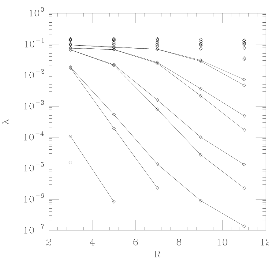
FIG. 1.: Low end of the positive half of the spectrum on a $L=32$ lattice on the special configuration as a function of $R$ which defines the area of constant magnetic field of flux $R$. Eigenvalues below $10^{-7}$ are not shown in this plot. Only for $R=3$ are all the eigenvalues above this bound. The lines connect eigenvalues at the same position in the ordering for each $R$.

What is the fermion spectrum in that case? The index theorem tells us that for a net flux $2\pi f$ through the area $L^{2}$, there are $f$ modes with zero eigenvalue. For $f=0$ and all boundary conditions periodic, there are two zero modes of the form above. But what else happens at the low end of the spectrum? There are two suggestions for an answer in the literature. The discussion of Casher and Neuberger [7] begins by dividing the $L\times L$ volume into $R\times R$-sized pieces with $gR$ and $L/R$ large. Considered in isolation, each of these areas has of order $gR$ zero modes. It is then argued that the effect of interaction between different regions is to shift the eigenvalues of the zero modes away from zero, in such a way as to produce a spectrum that is bounded below by one that is flat at small $\lambda$.

With a similar approach, Smilga [5] argues for a stronger lower bound that gives a spectral density that diverges as $\lambda\rightarrow 0$. His stronger result follows from using the fact that the value of the zero mode wave function on the boundary that separates a region with magnetic field from one with zero field is exponentially small in the flux through the region. Arguments using other methods in his paper and in the paper by Dürr and Sharpe [6] conclude that the divergence is quite strong with a factor $e^{cg^{2}V}$. This would be a consequence of modes with eigenvalues as small as the inverse of that factor.

For a numerical test of the argument used by Smilga to produce the stronger bound, we construct a background gauge field configuration that has two regions of size $R^{2}$ each with constant magnetic field and opposite net fluxes of magnitude $R$. We study the low lying eigenvalues of the overlap Dirac operator and show that they go down exponentially with $R$.

On the $L^{2}$ lattice, fix two regions of size $R^{2}$ separated by $(L/2-1,L/2-1)$. The slightly off-symmetric separation is chosen to avoid any accidental lattice symmetries. On one region of size $R^{2}$, we make up a constant magnetic field of flux $R$, and on the other region, we make up a constant magnetic field of flux $-R$. Elsewhere the field is zero. An initial numerical check with the field set to zero in one of the regions, verified the presence of $R$ topological zero modes for the overlap Dirac operator. Then returning to the case of interest with the field in both regions, we calculated the spectrum again. In Fig.1, we plot the low end of the positive half of the spectrum as a function of $R$. The lowest few of these small eigenvalues go down exponentially in $R$. We verified that this behavior remains unchanged when small random perturbations are added to the link elements. The numerical results are less restrictive than the theoretical arguments in that they do not rely on a variational argument, which without further work, applies only to a single mode on the lattice. Also all the lattice modes in addition to the would-be-zeros are included. This confirms the crucial point in the argument for the stronger bound of Ref.[5]. However, it does not provide evidence that the spacings might be as small as $e^{-cg^{2}V}$.

Let us now consider the continuum limit. Given the remark above on the lack of correlation in the field strengths, it is not possible to use a scale from that in defining the continuum. However, there is another simple approach. For $g$ small, ask how large does $R$ have to be so that the typical flux through the $R\times R$ area is of order one? Since the flux variance for a single plaquette is $g^{2}$ and the uncorrelated fluxes add, the variance for the area is $g^{2}R^{2}$. Thus the typical flux through the area is $gR$, and $g$ sets an inverse length or energy scale. This happens to be of the same order as the scale for the unquenched Schwinger model, in which the mass in lattice units is $g/\sqrt{\pi}$. We may hope to get a sensible continuum limit by measuring continuum dimensionful quantities in units of appropriate powers of $g/a$. To get the finite volume continuum limit, we will want to take $g$ to zero and $L$ to infinity with $gL$ fixed. Lattice eigenvalues, $<\bar{\psi}\psi>$, and other quantities with continuum units of energy should be considered in ratios like $\lambda/g$ as $g\rightarrow 0$.

Finally, let us discuss the range of $g$ and $L$ where these interesting effects might be seen. From two points of view, we can see that $gL$ must be large. First if $L$ is fixed and $g$ is small, then there are only perturbative effects from the gauge field, and the strong infrared fluctuations cannot appear. Also if $gL$ is small, then there are essentially no would-be-zero modes that could realize the the physical pictures of [7] and [5]. If $g$ is large, then the gauge field is very rough on the scale of a single lattice spacing, and the continuum-based arguments above do not apply. The smallest region that typically contains a unit of flux should be several lattice units so that it is large enough for the fermion to realize zero modes from the non-zero flux. Thus we must have $g$ small and $gL$ large, which means, of course, that $L$ must be large.

IV Numerical results

FIG. 2.: Plot of $<\bar{\psi}\psi>$ with respect to $m$ at $g=0.4\sqrt{\pi}$ for four different lattice sizes

FIG. 3.: Plot of the distribution of the small non-zero eigenvalues at $g=0.4\sqrt{\pi}$ for four different lattice sizes

The numerical results described in this section give substantial evidence that the infinite volume limit of the spectral density $\rho(\lambda)$ is indeed infinite for $\lambda\rightarrow 0$. We will show this by computing the spectrum of the overlap Dirac operator in U(1) gauge field backgrounds. The massless limit is approached in the conventional way by adding a standard mass term. We will also compute $<\bar{\psi}\psi>$ as a function of mass in finite lattice volumes and show that it grows as the mass is lowered before it finally dives to zero as it must for $m=0$ and finite volume. We will also show that the average value of the lowest eigenvalue does not scale with the volume, nor does it fit predictions from chiral random matrix theory.

Strong evidence for a divergence in the non-topological piece of $<\bar{\psi}\psi>$ is seen by plotting the gauge ensemble average of the second term in (2) as a function of $m$ at a fixed $g=0.4\sqrt{\pi}$ for several lattice sizes. We focus on the small mass region in Fig.2. The data at $L=32$ show a rise in $<\bar{\psi}\psi>$ as the mass is decreased. This divergence is due to an accumulation of very small eigenvalues at larger $L$ as seen in the histogram of the small non-zero eigenvalues in Fig.3. Even though only $L=32$ shows a rise in $<\bar{\psi}\psi>$ at small masses, an anomalous accumulation of very small eigenvalues is evident at $L=24$ in Fig.3. The accumulation is not enough to give a rise in $<\bar{\psi}\psi>$ on the $L=24$ lattice.

FIG. 4.: Plot of the distribution of the smallest eigenvalue scaled with the volume and restricted to the zero topological sector at $g=0.4\sqrt{\pi}$ for four different lattice sizes.

FIG. 5.: Ensemble average of the smallest eigenvalue in the zero and unit topological sectors at $g=0.4\sqrt{\pi}$ as a function of the lattice size and plotted to facilitate comparison with the simple functional forms described in the text.

The smallest eigenvalue $\lambda_{\rm min}$ has to scale like $1/V$ for a finite value of the density of eigenvalues at zero $\rho(0)$ and a finite value of $<\bar{\psi}\psi>$ in the massless limit. In Fig.4, we plot the histogram of $\lambda_{\rm min}L^{2}$ for the various ensembles in the zero topological sector. We see that there is no evidence for scaling in the distribution, whereas chiral random matrix theory predicts a universal function of the form ${z\over 2}e^{-{z^{2}\over 4}}$ with $z=\Sigma L^{2}\lambda_{\rm min}$ and $\Sigma$ the value of the chiral condensate. A previous analysis [12] of the distribution of the low lying eigenvalues done at smaller physical volume showed that the distribution did not fit the predictions of unitary chiral random matrix theory [13]. In Ref. [12] this was attributed to finite volume effects. In our case, the reason for the discrepancy is not small volumes but a divergent chiral condensate. Now consider the average of the smallest nonzero eigenvalue as a function of $L$. Three simple functions motivated by heuristic physics arguments are $c/V$, $e^{-cL}$, and $e^{-cV}$. To determine which of these forms is closest to the data, we have plotted in Fig.5 $V\langle\lambda_{\rm min}\rangle/16$, $\ln(\langle\lambda_{\rm min}\rangle/\langle\lambda_{\rm min}\rangle\mid_{L=8})/(8-L)$, and $50\ln(\langle\lambda_{\rm min}\rangle/\langle\lambda_{\rm min}\rangle\mid_{L=8})/(64-V)$ verses $L$ for $Q=0$ and $|Q|=1$. (The normalizations are just for convenience.) To the extent that one of these functions represents the data well, the corresponding graph in Fig.5 should be flat. Evidently $e^{-cL}$ is preferred. Recall that this is the form that appears in the argument for the lower bound in [5] and in the spectrum from the artificial configurations described in Section III.

FIG. 6.: Plot of $<\bar{\psi}\psi>/g$ with respect to $m/g$ at $gL/\sqrt{\pi}=12.8$ on $L=24,28,32$.

FIG. 7.: Plot of $<\bar{\psi}\psi>/g$ with respect to $m/g$ at $L=32$ and four different couplings.

Fig.2 shows that $L=32$ is needed at $g=0.4\sqrt{\pi}$ to see the divergent behavior in the chiral condensate. This corresponds to a physical volume of $gL/\sqrt{\pi}=12.8$. To study the effect of lattice spacing, we compared this result with others obtained on $L=24$ at $g/\sqrt{\pi}=0.4(32/24)$ and on $L=28$ at $g/\sqrt{\pi}=0.4(32/28)$. These have the same physical volume $gL/\sqrt{\pi}=12.8$ but are coarser lattices. The comparison in Fig.6 shows that the divergence visible on the $L=32$ lattice is not seen on the $L=24$ lattice. However, the $L=28$ data follow the $L=32$ data to very small masses and into the region where the condensate begins to grow. We have used dimensionless quantities in this plot to facilitate a proper comparison. The scaling behavior is good until $m/g$ gets small enough to emphasize the very smallest eigenvalues, some of which are being distorted on the coarser lattice. At smaller coupling and at the same physical volume, the scaling behavior extends to smaller $m/g$.

To illustrate the point that at fixed $L$, $g$ can be neither too big nor too small if the small $\lambda$ growth is to be seen, we have data from $L=32$ and four couplings in Fig.7. The smallest value of $g$, which corresponds to a physical size of 9.6, shows no growth at all. The medium values at sizes 12.8 and 16 show the effect. (Note that the finite size effects between these two are small.) The largest value of $g$ has size 32 but the gauge field there is too rough, and the small $\lambda$ peak is gone.

V Conclusions

We have shown that for small coupling and large volume, a small eigenvalue peak appears in the spectral density of the overlap Dirac operator and in $<\bar{\psi}\psi>$. This is strong evidence for the predictions [5, 6] that these quantities diverge in the infinite volume limit of the quenched Schwinger model. There is some evidence that the divergence could be as strong as $e^{cgL}$, but the lattice sizes are insufficient to provide evidence for the stronger $e^{dg^{2}L^{2}}$ predictions. Similarly there is limited evidence that the would-be-zero modes of subregions of the lattice can provide a physical understanding of the results. However, a definite test of that model also awaits data from larger lattices.

The results in this paper clearly point the direction for further work. The calculations should be extended to larger lattices so that there are several sizes showing the small $\lambda$ growth of the spectral density and $<\bar{\psi}\psi>$. With that, it would be possible to study the volume dependence of the small $\lambda$ peaks and test in more detail the theoretical expectations.

Although the quenched Schwinger model is quite some distance from full four-dimensional QCD, results from it help to map out the range of territory available to massless fermions responding to a gauge field.

- [1] C. Bernard and M. Golterman, Phys. Rev. D 46, 853 (1992); S. Sharpe, Phys. Rev. D 46, 3146 (1992).
- [2] H. Thacker, W. Bardeen, A. Duncan and E. Eichten, Nucl. Phys. Proc. Suppl. 73 (1999) 243; CP-PACS Collaboration (S. Aoki et al.), Phys. Rev. Lett. 84 (2000) 238.
- [3] U. Sharan and M. Teper, hep-ph/9910216.
- [4] J. Lowenstein and J. Swieca, Ann. Phys. 68, 172 (1961).
- [5] A.V. Smilga, Phys. Rev. D 46, 5598 (1992).
- [6] S. Dürr and S.R. Sharpe, hep-lat/9902007.
- [7] A. Casher and H. Neuberger, Phys. Lett. B139, 67 (1984).
- [8] H. Neuberger, Phys. Lett. B417, 141 (1998).
- [9] R.G. Edwards, U.M. Heller, and R. Narayanan, Phys. Rev. D 59, 094510 (1999).
- [10] R. Narayanan and H. Neuberger, Phys. Rev. Lett. 71, 3251 (1993).
- [11] G. ’t Hooft, Phys. Rev. Lett. 37, 8 (1976); Phys. Rev. D14, 3432 (1976).
- [12] F. Farchioni, I. Hip, C.B. Lang and M. Wohlgenannt, Nucl. Phys. B549, 364 (1999).
- [13] The recent paper M. Schnabel and T. Wettig, hep-lat/9912057 offers an explanation of the disagreement observed in Ref. [12] by arguing that the cause is a zero chiral condensate at finite volume in the quenched Schwinger model. This is supported by some numerical computations. While the model in hep-lat/9912057 is interesting, the action they used is not gauge invariant, and it does not give an area law for the Wilson loop. Therefore there is some question about the relevance of the calculation to the quenched Schwinger model.