Towards a Many-Body Treatment of Hamiltonian Lattice ${SU}(N)$ Gauge Theory

Abstract

We develop a consistent approach to Hamiltonian lattice gauge theory, using the maximal-tree gauge. The various constraints are discussed and implemented. An independent and complete set of variables for the colourless sector is determined. A general scheme to construct the eigenstates of the electric energy operator using a symbolic method is described. It is shown how the one-plaquette problem can be mapped onto a $N$-fermion problem. Explicit solutions for $U(1$), $SU(2)$, $SU(3)$, $SU(4)$, and $SU(5)$ lattice gauge theory are shown.

Contents

• Introduction.

• Hamiltonian lattice gauge theory. 2.1. Discretisation. 2.2. Gauss’ law.

• Explicit Hamiltonian. 3.1. Conditions on variables. 3.2. The gauge-fixed Hamiltonian. 3.3. Boundaries.

• Further constraints.

• The one-plaquette problem. 5.1. Angular representation. 5.2. $\operatorname{Tr}[U]$ as a raising operator. 5.3. The harmonic approximation. 5.4. Large-$N$ limit. 5.5. Explicit solutions.

• Wave functionals.

• Conclusions.

• One-dimensional many-fermion systems and their representations A.1 The magnetic term.

• Equivalent forms of the electric energy.

1 Introduction

Strongly interacting gauge-field theories, where perturbation theory is of no help, have been a long-standing problem. The theory of strong interactions, quantum-chromodynamics (QCD), is probably the most well-known theory of this type. This paper is concerned with one approach to such problems, the Hamiltonian description of the lattice version of gauge-field theory (LGFT). For most investigations in this area this is not the method of choice; the majority of calculations on such theories are done within the Lagrangian formalism. The main reason for this is the fact that, at least in principle, the Lagrangian method is elegant and simple. It is based on a path-integral approach to the imaginary-time propagation. Much work has been done to improve the accuracy of the Monte Carlo method used in the numerical implementation of the Lagrangian approach, further increasing the viability of the method.

Thus, anyone wishing to pursue a different path needs first to build a strong case for the merits of their approach. For the form of the Hamiltonian approach we shall consider in this paper we see four important advantages:

1. The Lagrangian approach, being based on an imaginary time evolution, does not allow easy access to the vacuum wave functional. By contrast, in the Hamiltonian approach such a wave functional is at the core of the calculation, and we cannot avoid to calculate it. Once the vacuum wave functional is known, most properties of theories such as QCD, like confinement and chiral symmetry breaking, should follow automatically.

2. Time-dependent phenomena can only be discussed in a real time (Hamiltonian) setting.

3. The physical interpretation of the variables is more transparent. For example, electric and magnetic operators have their classical meaning.

4. The Hamiltonian approach can studied not only with numerical, but also with analytical techniques, so we can study low-lying excitations with a harmonic approximation and we can disentangle the dependence of observables on the parameters in the approximation.

These advantages are accompanied by important disadvantages. Due to the fact that the Hamiltonian requires a quantisation plane to be defined, we lose the manifest Lorentz symmetry, that arises so naturally in the Lagrangian approach. In the full solution to the Hamiltonian problem this should be recovered, but approximations can introduce spuriosities. Furthermore we have to fix the gauge, and the degrees of freedom in the Hamiltonian formulation of the theory will then naturally depend on the choice of gauge. The issue of gauge fixing is a rather non-trivial exercise, as we shall see in this paper.

We shall first, in Sec. 2, give a short introduction to our version of lattice gauge theory. In Sec. 3 we then discuss how we can use the idea of a maximal tree to define a fully gauge-fixed Hamiltonian, which is derived in an explicit form. In Sec. 4 we discuss those constraints relating the trace of powers of $SU(N)$ matrices, and we define a symbolic method to construct eigenvalues of the electric energy operator, which should be useful in any approach to Hamiltonian LGFT. We then study the one plaquette problem in Sec. 5, first in its generality, showing how we can derive a simple $N$-fermion problem equivalent to the $SU(N)$ one-plaquette problem. We discuss both the weak-coupling (harmonic) and the large-$N$ limits. Explicit results for the one plaquette spectra as function of the coupling constant are shown for $U(1)$, and $SU(N)$ LGFT’s, with $2\leq N\leq 5$. Finally we discuss the results and future directions in Sec. 7.

2 Hamiltonian lattice gauge theory

The degrees of freedom in a gauge theory, such as electromagnetism, can be divided into two sets. The first set consists of the charges and currents in the system together with the associated static electric and magnetic fields. The second set contains the electromagnetic waves. However, since a charge in a moving frame is a current, relativistic coordinate transformations mix electric and magnetic variables. Moreover, since the velocity of electromagnetic waves is constant, the two polarisation directions, perpendicular to the propagation direction, also undergo complicated transformations under a change of frame. Therefore a relativistically invariant formulation of electromagnetism is very useful.

As is well known, the Lagrangian of electromagnetism, without static sources,

$$\mathcal{L}=\frac{1}{2}\sum_{i=1}^{3}(E_{i}^{2}-B_{i}^{2})\quad,$$ (1)

can be formulated in terms of a covariant four-vector potential $A_{\mu}$ as

$$\mathcal{L}=\frac{1}{4}(\partial_{\mu}A_{\nu}-\partial_{\mu}A_{\nu})^{2}\quad,$$ (2)

where $B_{i}=\epsilon_{ijk}\partial_{j}A_{k}$ and $E_{i}=\partial_{i}A_{0}-\partial_{0}A_{i}$. We use a notation in which roman indices $i,j,k,\ldots$ run over the spatial, while greek indices $\mu,\nu,\ldots$ run over the values $0,1,2,\ldots,D$, where $D$ is the number of space dimensions and the temporal axis has index 0. The introduction of the vector potential, or gauge field, serves a number of purposes. Firstly, since the gauge field transforms as a vector, the Lagrangian is now manifestly relativistically invariant. Secondly, it is formulated in terms of canonical variables $A_{\mu}$ and $\partial_{0}A_{\mu}$ which should make quantisation more straightforward; and thirdly, the two constraints for the electric and the magnetic fields, the source-free Maxwell equations $\partial_{i}B_{i}=0$ and $\partial_{0}B_{i}=-\epsilon_{ijk}\partial_{j}E_{k}$, are automatically satisfied. The price we pay for this is the appearance of superfluous degrees of freedom, the gauge, and an entanglement of the sources giving rise to these variables.

The original Abelian gauge theory of electromagnetism was extended by Yang and Mills [1] using gauge fields of more complicated structure, including internal degrees of freedom. This generates self-interactions since the gauge fields do not commute, but are chosen to obey the commutation relations of a specific Lie algebra. We shall concentrate on a gauge-field Lagrangian where the field $\boldsymbol{A}_{\mu}$ is an element of the Lie algebra ${su}(N)$,

$$\mathcal{L}=\frac{1}{2g^{2}}\operatorname{Tr}[\boldsymbol{F}_{\mu\nu}\boldsymbol{F}^{\mu\nu}]\quad.$$ (3)

Here the field tensor is the skew-Hermitian matrix $\boldsymbol{F}_{\mu\nu}\equiv\partial_{\mu}\boldsymbol{A}_{\nu}-\partial_{\nu}\boldsymbol{A}_{\mu}-i[\boldsymbol{A}_{\mu},\boldsymbol{A}_{\nu}]$, and the field variable $\boldsymbol{A}_{\mu}$ is an element of the algebra, conveniently parametrised as

$$\boldsymbol{A}_{\mu}\equiv g\frac{1}{2}\lambda^{a}A^{a}_{\mu}\quad.$$ (4)

The $\lambda^{a}$ are the $N^{2}-1$ generators of the Lie algebra, satisfying the commutation relations

$$[\lambda^{a},\lambda^{b}]={2}if^{abc}\lambda^{c}\quad.$$ (5)

The index $a$ thus runs from $1$ to $N^{2}-1$. The $\lambda^{a}$ can be represented by traceless $N\times N$ matrices, normalised such that their squares have trace 2, as can be seen from the anticommutation relations

$$\{\lambda^{a},\lambda^{b}\}={2}d^{abc}\lambda^{c}+\frac{4}{N}\delta_{ab}I\quad.$$ (6)

In Eq. (4) we have absorbed the coupling constant $g$ in the field $\boldsymbol{A}_{\mu}$, so that we can interpret the fields geometrically, since the field tensor is now the curvature that follows from the covariant derivative

$$\boldsymbol{d}_{\mu}\equiv\partial_{\mu}-i[\boldsymbol{A}_{\mu},\cdot]\quad,$$ (7)

i.e.,

$$[\boldsymbol{d}_{\mu},\boldsymbol{d}_{\nu}]=[\boldsymbol{F}_{\mu\nu},\cdot]\quad.$$ (8)

As we are interested in the Hamiltonian, we perform the standard equal-time quantisation and reformulate the Lagrangian in generalised electric and magnetic fields. This is strictly speaking a 3-dimensional result, since this interpretation requires the use of three-dimensional algebra. We shall nonetheless use the result below for other dimensions as well. We find

$$\mathcal{L}=\frac{1}{g^{2}}\operatorname{Tr}\left[\sum_{k=1}^{D}(\boldsymbol{E}_{k}^{2}-\boldsymbol{B}_{k}^{2})\right]\quad,$$ (9)

where $\boldsymbol{B}_{i}=-\frac{1}{2}\epsilon_{ijk}\boldsymbol{F}_{jk}$ and $\boldsymbol{E}_{i}=\boldsymbol{F}_{i0}$. Since we wish to impose the temporal gauge $\boldsymbol{A}_{0}=0$, we separate the Hamiltonian in two parts, thereby isolating the $\boldsymbol{A}_{0}$ dependent part: [2]

$$\mathcal{L}=\frac{1}{g^{2}}\operatorname{Tr}\left[\sum_{k=1}^{D}(\boldsymbol{E}_{k}^{2}-\boldsymbol{B}_{k}^{2})\right]_{\boldsymbol{A}_{0}=0}+\frac{1}{g^{2}}\operatorname{Tr}\left[\boldsymbol{A}_{0}\boldsymbol{\mathcal{G}}+\boldsymbol{A}_{0}\boldsymbol{\mathcal{X}}(\boldsymbol{A}_{0})\right]\quad,$$ (10)

where we added a total divergence. The function $\boldsymbol{\mathcal{X}}$ is second order in $\boldsymbol{A}_{0}$ and does not contribute to the equations of motion, or the constraint equations in the temporal gauge (${\boldsymbol{A}}_{0}=0$) discussed below. Since the time-derivative of $\boldsymbol{A}_{0}$ does not occur in the Lagrangian, the (Lagrangian) extremal action variational principle leads to an equation of motion for $\boldsymbol{A}_{0}$ that is a time-independent algebraic equation, which shows that the $\boldsymbol{A}_{0}$ takes on a time-independent constant value. This set of equations (one for each colour index) are the non-Abelian analogue of the Gauss’ law constraint, which in the absence of colour charges take the simple form

$${\mathcal{G}}^{a}(\mathbf{x})=0\quad,$$ (11)

where

$${\mathcal{G}}^{a}(\mathbf{x})=\sum_{i=1}^{D}[\partial_{i}E^{a}_{i}(\mathbf{x})+gf^{abc}A_{i}^{b}(\mathbf{x})E_{i}^{c}(\mathbf{x})]=\sum_{i=1}^{D}\boldsymbol{d}_{i}E_{i}^{a}\quad.$$ (12)

The components of the fields can be obtained via the relation

$$A^{a}_{\mu}=\frac{1}{g}\operatorname{Tr}[\boldsymbol{A}_{\mu}\lambda^{a}],\quad E^{a}_{\mu}=\frac{1}{g}\operatorname{Tr}[\boldsymbol{E}_{\mu}\lambda^{a}]\quad.$$ (13)

The constraints obey the same commutation relations as the generators of the gauge group. Thus Gauss’ law cannot be implemented as a strict operator condition as it leads to contradictions, since the non-commuting constraints cannot all be diagonalised simultaneously. However, within the physical (in this case colourless) subspace defined by

$$\mathcal{G}^{a}(\mathbf{x})|\mathrm{Phys}\rangle=0\quad,$$ (14)

no such problem arises, since the eigenvalue of the commutators is also $0$. The space of states consists of wave functionals, which are functionals taking values on the $SU(N)$ group manifold. We find $N^{2}-1$ functional conditions on each wave functional, consisting of functions on the group manifold at each space point.

As is well known, quantisation of problems involving redundant degrees of freedom (i.e., where some of the equations of motion are constraints) is quite involved. The two main techniques used are Dirac and BRS quantisation, and they require a large amount of additional analysis. For more details one can consult the seminal work by Dirac [3, 4], as well as Refs. [2, 5, 6, 7, 8].

If we are able to work within the physical subspace only, one can ignore these formal problems and define the quantisation of the canonical momenta $\Pi_{i}^{a}=\partial_{0}A_{a}^{i}$ by

$$\Pi^{a}_{i}(\mathbf{x})=\hat{E}_{i}^{a}=-i\frac{\delta}{\delta A_{i}^{a}(\mathbf{x})}\quad,$$ (15)

which involves a functional derivative [9, 10] with respect to the field variables.

Since $A^{a}_{0}$ is not dynamical, we cannot associate a canonical momentum with it. We therefore use the temporal gauge, $A^{a}_{0}=0$, which leaves us with residual gauge freedom $\boldsymbol{\phi}(\mathbf{x})$ independent of the time coordinate, i.e., under the transformation

$${}^{\boldsymbol{\phi}}\boldsymbol{A}_{\mu}(\mathbf{x}) = \boldsymbol{\phi}(\mathbf{x})\boldsymbol{A}_{\mu}(\mathbf{x})\boldsymbol{\phi}^{-1}(\mathbf{x})+i[\partial_{\mu}\boldsymbol{\phi}(\mathbf{x})]\boldsymbol{\phi}^{-1}(\mathbf{x})\quad,$$ (16)

$${}^{\boldsymbol{\phi}}\boldsymbol{F}_{\mu\nu}(\mathbf{x}) = \boldsymbol{\phi}(\mathbf{x})\boldsymbol{F}_{\mu\nu}(\mathbf{x})\boldsymbol{\phi}^{-1}(\mathbf{x})\quad,$$ (17)

where $\boldsymbol{\phi}\in SU(N)$, the Lagrangian is invariant.

2.1 Discretisation

Field theories suffer from singularities, both in the infrared and ultraviolet limits. In many interesting cases, such as QCD [11], these are renormalisable. Rather than dealing directly with the continuum, we shall regularise the problem by introducing a simple hypercubic lattice in the $D$-dimensional space, with lattice spacing $a$. Since we are pursuing a Hamiltonian approach, time will remain continuous. In this paper we shall concentrate on pure gauge theory, without explicit charges (i.e., quarks). In this case the systems is described by a set of gauge fields $A^{a}_{i}$ at each point of the $D$-dimensional lattice. It looks like these could in principle carry $D(N^{2}-1)$ degrees of freedom, as the group ${SU}(N)$ has $N^{2}-1$ generators $\lambda^{a}$. However, even after restricting the gauge fields by imposing the temporal gauge $\boldsymbol{A}_{0}=0$, the Lagrangian is still invariant under a limited set of gauge transformations that do not violate the temporal constraint. Thus the apparent number of degrees of freedom is still larger than that required to specify the dynamics uniquely. These superfluous degrees of freedom arise since we have not fully exploited the Gauss’ law constraints.

In order to analyse this problem fully we first investigate the structure of the Hamiltonian on the lattice. The gauge fields

$$\boldsymbol{A}_{i}=g\frac{1}{2}\sum_{a=1}^{N^{2}-1}\lambda^{a}A^{a}_{i}\quad,$$ (18)

are Hermitian, since $\lambda^{a}$ is Hermitian. In the Schrödinger (wave function) representation the effect of these fields can be incorporated as a non-Abelian change of phase of the wave function between different points, a simple generalisation of the Aharonov-Bohm effect in QED. This geometric interpretation can be represented by a group element, a unitary transformation summing all the small phase changes along the path connecting the two points,

$$U(\mathbf{x}_{1},\mathbf{x}_{2})\equiv P\exp\left\{i\int_{\mathbf{x}_{1}}^{\mathbf{x}_{2}}\boldsymbol{A}_{\mu}(\mathbf{x})dx^{\mu}\right\}\quad,$$ (19)

where we have introduced a path-ordered product, denoted by $P$, since the quantities $\boldsymbol{A}_{\mu}(\mathbf{x})$ for different values of $\mathbf{x}$ are non-commuting matrices.

In practice we will only use this unitary transformation (which for obvious reasons is also called a parallel transporter) on a link between two nearest-neighbour lattice points $\mathbf{i}$ and $\mathbf{j}$ where $\mathbf{a}_{\mu}=\mathbf{x}_{\mathbf{i}}-\mathbf{x}_{\mathbf{j}}$ is a primitive lattice vector in the direction $\mu$ (we shall use the bracket notation $\langle\rangle$ to denote nearest-neighbour pairs)

$$U_{\langle\mathbf{i}\mathbf{j}\rangle} = P\exp\left\{i\int_{\mathbf{x}_{\mathbf{i}}}^{\mathbf{x}_{\mathbf{j}}}\boldsymbol{A}_{\mu}(\mathbf{x})dx^{\mu}\right\}\equiv\exp\left\{ia_{\mu}\overline{\boldsymbol{A}}_{\mu}(\mathbf{x}_{\langle\mathbf{i}\mathbf{j}\rangle})\right\}\quad,$$ (20)

$$U_{\langle\mathbf{j}\mathbf{i}\rangle} = \exp\left\{-ia_{\mu}\overline{\boldsymbol{A}}_{\mu}(\mathbf{x}_{\langle\mathbf{i}\mathbf{j}\rangle})\right\}=U^{\dagger}_{\langle\mathbf{i}\mathbf{j}\rangle}\quad.$$ (21)

In Eq. (20) we have defined $\overline{\boldsymbol{A}}_{\mu}$ at the midpoints of the link,

$$\mathbf{x}_{\langle\mathbf{i}\mathbf{j}\rangle}=\frac{1}{2}(\mathbf{x}_{\mathbf{i}}+\mathbf{x}_{\mathbf{j}})\quad.$$ (22)

Since $\boldsymbol{A}_{\mu}$ is an element of the ${su}(N)$ Lie algebra, $U$ is a ${SU}(N)$ matrix, and satisfies $U^{-1}=U^{\dagger}$ and $\det U=1$. The quantity $\overline{\boldsymbol{A}}_{\mu}(\mathbf{x}_{\langle\mathbf{i}\mathbf{j}\rangle})$ is a geometrical average of $\boldsymbol{A}_{\mu}$ along the link $\langle\mathbf{i}\mathbf{j}\rangle$ in direction $\mu$. Since all future discussions will only concern this averaged field, we suppress the bar from here onwards.

Figure 1: The path for the elementary plaquette.

The four links around a primitive square (usually called plaquette) on the lattice will give, when we take the trace, the simplest gauge-invariant quantity on the lattice, and for that reason is often used in lattice problems. As an example we take a plaquette in the $xy$ plane, $(0,0)\rightarrow(a_{x},0)\rightarrow(a_{x},a_{y})\rightarrow(0,a_{y})\rightarrow(0,0)$, see Fig. 1. This leads to (the notation $\mathbf{a}_{i}$ is used as a shorthand for $a_{i}$ times a unit vector in the direction $i$)

$$U_{\square} = e^{ia_{x}\boldsymbol{A}_{x}(\mathbf{a}_{x}/2)}e^{ia_{y}\boldsymbol{A}_{y}(\mathbf{a}_{x}+\mathbf{a}_{y}/2)}e^{-ia_{x}\boldsymbol{A}_{x}(\mathbf{a}_{y}+\mathbf{a}_{x}/2)}e^{-ia_{y}\boldsymbol{A}_{y}(\mathbf{a}_{y}/2)}$$ (23)

$$= \exp\left\{ia_{x}a_{y}\left(\Delta_{y}\boldsymbol{A}_{x}(\mathbf{m})-\Delta_{x}\boldsymbol{A}_{y}(\mathbf{m})-[\boldsymbol{A}_{x}(\mathbf{m}),\boldsymbol{A}_{y}(\mathbf{m})]\right)+{\mathcal{O}}(a^{3}\right\}\quad,$$

where $\mathbf{m}=(\mathbf{a}_{x}+\mathbf{a}_{y})/2$ is the centre of the plaquette, and we have assumed that both $a_{x}$ and $a_{y}$ are of order $a$. We have used the Campbell-Baker-Hausdorff formula to combine the exponentials,

$$\exp(A)\exp(B)=\exp\left\{A+B+\frac{1}{2}[A,B]+\frac{1}{12}[A,[A,B]]+\frac{1}{12}[[A,B],B]+\cdots\right\}\quad.$$ (24)

The operator $\Delta_{i}$ is the lattice derivative, defined as

$$\Delta_{i}\boldsymbol{A}_{j}(\mathbf{m})=\frac{\boldsymbol{A}_{j}(\mathbf{m}+\mathbf{a}_{i}/2)-\boldsymbol{A}_{j}(\mathbf{m}-\mathbf{a}_{i}/2)}{a_{i}}\quad.$$ (25)

Eventually we find, using $a_{x}=a_{y}=a$,

$$U=e^{-a^{2}i\boldsymbol{F}_{xy}+{\mathcal{O}}(a^{3})}\quad.$$ (26)

We would like to associate the trace of $U$ with a lattice version of the QCD Lagrangian. The requirement is that in the $a\rightarrow 0$ limit the Lagrangian becomes the continuum one. Thus we must analyze the expansion of the trace. If we expand $U_{\square}$ in a Taylor series in $a$, we find that the $a^{2}$ and $a^{3}$ terms are traceless, and so are all the terms of the order $a^{4}$ except for the term $-i(\boldsymbol{F}_{xy})^{2}$. Thus it seems natural to define $\operatorname{Tr}U_{\square}$ as the lattice potential. Unfortunately, this is a complex quantity, and we need to combine it with its complex conjugate to get a real result,

$$\frac{1}{2a^{4}g^{2}}\operatorname{Tr}[\boldsymbol{F}_{xy}\boldsymbol{F}_{xy}]=\frac{1}{2a^{4}g^{2}}\operatorname{Tr}[2-U_{\square}-U_{\square}^{-1}]+{\mathcal{O}}(a)\quad.$$ (27)

Clearly this approaches the continuum result as $a\rightarrow 0$. This is the one-plaquette contribution to the magnetic part of the Wilson action [12, 13].

In a Hamiltonian formalism we need to construct canonical momenta. The natural choice is the differential realisation of the generators at each lattice point (i.e., the generalised angular momentum operators for the group ${SU}(N)$). These act naturally on the original lattice variables $\boldsymbol{A}_{\mu}(\mathbf{x}_{\mathbf{i}})$, but as stated above we really would like to formulate the problem in terms of link variables $U_{\langle\mathbf{i}\mathbf{j}\rangle}$. Using the definition of $U_{\langle\mathbf{i}\mathbf{j}\rangle}$ as a path-ordered product, Eq. (19), we find that the action of the momenta, conventionally called electric fields $E$, is given by

$$E_{\mu}^{a}(\mathbf{x}_{\mathbf{i}})U_{\langle\mathbf{i}\mathbf{j}\rangle} = -\frac{1}{2}\lambda^{a}U_{\langle\mathbf{i}\mathbf{j}\rangle}\quad,$$

$$E_{\mu}^{a}(\mathbf{x}_{\mathbf{i}})U_{\langle\mathbf{j}\mathbf{i}\rangle} = \frac{1}{2}U_{\langle\mathbf{j}\mathbf{i}\rangle}\lambda^{a}\quad,$$ (28)

where $\mathbf{j}=\mathbf{i+e}_{\mu}$, so $\mu$ must point along the link $\langle\mathbf{i}\mathbf{j}\rangle$ in the positive direction. The second relation follows from the Hermitian conjugation. This can also be written as a differential operator acting on the link-averaged gauge fields $A^{a}_{\mu}(\mathbf{x}_{\langle\mathbf{i}\mathbf{j}\rangle})$,

$$E_{\mu}^{a}(x_{\mathbf{i}})=-\frac{i}{a_{\mu}}\frac{\delta}{\delta A^{a}_{\mu}(\langle\mathbf{x}_{\mathbf{i}\mathbf{j}}\rangle)}\delta_{\mathbf{x}_{\mathbf{j}}-\mathbf{x}_{\mathbf{i}},\mathbf{a}_{\mu}}\quad.$$ (29)

We shall also use the notation $E^{a}_{\mathbf{i}\mathbf{j}}$ for this same operator.

Ignoring problems with overcompleteness, we can derive the Kogut-Susskind Hamiltonian, [7]

$$H_{\mathrm{KS}} = \frac{g_{t}^{2}}{2a^{D-2}}\left(\sum_{\mathbf{i},\mu}^{Dn^{D}}\sum_{a=1}^{N^{2}-1}E_{\mu}^{a}(\mathbf{x}_{\mathbf{i}})E^{a}_{\mu}(\mathbf{x}_{\mathbf{i}})+\frac{1}{g^{3}_{t}g_{s}a^{6-2D}}\sum_{\langle\mathbf{i}\mathbf{j}\rangle}^{\frac{1}{2}D(D-1)n^{D}}\operatorname{Tr}[2-U(\mathbf{m}_{\mathbf{i},k,l})-U^{-1}(\mathbf{m}_{\mathbf{i},k,l})]\right)$$ (30)

$$= \frac{g_{t}^{2}}{2a^{D-2}}\left(H_{E}+\frac{1}{g^{3}_{t}g_{s}a^{6-2D}}H_{M}\right)\quad,$$

where $n$ is the length of the lattice, and $D$ is the number of space dimensions. The quantity $U(\mathbf{m}_{\mathbf{i},k,l})$ is the Wilson plaquette around the face centre $\mathbf{m}_{\mathbf{i}}$ in the directions $k$ and $l$,

$$U(\mathbf{m}_{\mathbf{i},k,l})=U_{\mathbf{i},(\mathbf{i}+\mathbf{a}_{k})}U_{(\mathbf{i}+\mathbf{a}_{k}),(\mathbf{i}+\mathbf{a}_{k}+\mathbf{a}_{l})}U_{(\mathbf{i}+\mathbf{a}_{k}+\mathbf{a}_{l}),(\mathbf{i}+\mathbf{a}_{l})}U_{(\mathbf{i}+\mathbf{a}_{l}),\mathbf{i}}\quad,$$ (31)

where $\mathbf{m}_{\mathbf{i}}=\mathbf{x}_{\mathbf{i}}+\frac{1}{2}(\mathbf{a}_{k}+\mathbf{a}_{l})$. We have written down the slightly more general form of Hamiltonian obtained when we realise that the coupling constants $g_{t}$ and $g_{s}$ for the spatial and time components of $\boldsymbol{A}$ can be different, since the Hamiltonian breaks manifest Lorentz invariance. In principle one has to solve a renormalisation problem to find the physical couplings that correspond to these bare ones, a problem that we shall not address in this paper.

2.2 Gauss’ law

The constraints, Eqs. (11,12), can also be interpreted as arising from the invariance of the gauge-fixed Lagrangian under residual gauge transformations $\boldsymbol{\phi}$. Unfortunately, the result (12) is only correct for continuum theories, since it involves the field $\boldsymbol{A}_{\mu}$ rather than its lattice analogue $U$. The derivation of Gauss’ law constraints on the lattice is discussed in Ref. [14]. The approach is based on the fact that a wave functional, which dependens on the overcomplete set of link variables,

$$\Psi(\{U\})\quad,$$ (32)

Should be invariant under a gauge transformation on a single lattice site,

$$U_{\mathbf{i},\mathbf{i}+e_{\mu}} \to e^{i\boldsymbol{\phi}_{\mathbf{i}}}U_{\mathbf{i},\mathbf{i}+e_{\mu}}e^{i\boldsymbol{\phi}^{\dagger}_{\mathbf{i}+e_{\mu}}}$$ (33)

$$U_{\mathbf{i}-e_{\mu},\mathbf{i}} \to e^{i\boldsymbol{\phi}_{\mathbf{i}-e_{\mu}}}U_{\mathbf{i}-e_{\mu},\mathbf{i}}e^{i\boldsymbol{\phi}^{\dagger}_{\mathbf{i}}}\quad.$$ (34)

The invariance can be written in terms of generators as

$$\exp\left[i\phi^{a}\sum_{\mu}^{D}(E^{a}_{i,\mu}-E^{(L)}_{i,\mu})\right]\Psi(\{U\})=0\quad,$$ (35)

where $E^{(L)a}$ are the left-handed generator for $SU(N)$,

$$E^{(L)a}_{\mathbf{i},\mu}U_{\mathbf{i}-e_{\mu},\mathbf{i}}=U_{\mathbf{i}-e_{\mu},\mathbf{i}}\left(\frac{1}{2}\lambda^{a}\right)\quad,$$ (36)

which give rise to the right-multiplication in Eq. (34).

From the infinitesimal from of Eq. (35 we find the lattice form of the Gauss’ law,

$$\sum_{\mu}^{D}(E^{a}_{i,\mu}-E^{(L)}_{i,\mu})\Psi(\{U\})=0\quad.$$ (37)

It is easy to show that

$$E^{(L)a}_{\mathbf{i},\mu} = D_{ab}(U_{\mathbf{i}-e_{\mu},\mathbf{i}})E^{a}_{\mathbf{i},\mu}\quad,$$ (38)

$$D_{ab}(U) = \frac{1}{2}\operatorname{Tr}\left[U\lambda^{a}U^{\dagger}\lambda^{b}\right]\quad,$$ (39)

$$\,[E^{(L)a}_{\mathbf{i},\mu},E^{(L)b}_{\mathbf{i},\mu}] = -2if^{abc}E^{(L)c}_{\mathbf{i},\mu}\quad.$$ (40)

We thus find the lattice version of the Gauss’ law generators

$$G^{a}_{\mathbf{i},\mu}=\left(E^{a}_{\mathbf{i},\mu}-D_{ab}(U_{\mathbf{i}-e_{\mu},\mathbf{i}})E^{a}_{\mathbf{i}-e_{\mu},\mu}\right)\quad.)$$ (41)

In the limit that the lattice spacing vanishes this simplifies to the original Gauss’ law generator, Eq. (12).

From Eq. (41) we see that we can define a covariant lattice derivative, which takes the matrix form

$$\boldsymbol{D}_{\mathbf{i},\mathbf{j},\mu}=\delta_{\mathbf{i}+e_{\mu},\mathbf{j}}-D_{ab}(U_{\mathbf{i}-e_{\mu},\mathbf{i}})\delta_{\mathbf{i}-e_{\mu},\mathbf{j}}\quad.$$ (42)

This construction of the Gauss’ law makes it clear why it is so attractive to work with functions of traces of the product of $U$ along closed loops (Wilson loops), since those varaibles are automatically gauge invariant.

Table 1: The number of degrees of freedom on a hypercubic lattice of size $n\times n\times\cdots n$, for different numbers of space dimensions. The $D=1$ case comprises $n$ plaquettes on a line

dimensionality	“1”	2	3	$D$
number of sites	$2(n+1)$	$(n+1)^{2}$	$(n+1)^{3}$	$(n+1)^{D}$
number of links	$3n+1$	$2n(n+1)$	$3n(n+1)^{2}$	$Dn(n+1)^{D-1}$
number of plaquettes	$n$	$n^{2}$	$3n^{3}$	$\frac{1}{2}D(D-1)n^{D}$

Thus the number of constraints equals the number of group generators times the number of sites, and the number of degrees of freedom equals the number of generators times the number of links. The number of unconstrained degrees of freedom is clearly the latter number minus the former. As shown in Table 1, for one and two space dimensions, in the limit of infinite extent, this is exactly the number of plaquettes times the number of gauge degrees of freedom. This is not true in higher dimensions, and we shall have to do some more work to get around this problem.

Another interpretation of this procedure is that Gauss’ law fixes the longitudinal electric field. This field is a direct consequence of the charge density distribution in the system. Since we will work in the colourless sector, the longitudinal field is zero, in agreement with our results above.

3 Explicit Hamiltonian

The link variables are a sufficient set of variables, and, when combined in closed contours, they are gauge invariant. This means that projections on the colour-neutral sector by integration over the gauge group, as seen in many Lagrangian lattice gauge approaches to the problem, have no effect. The price we have paid for the Hamiltonian approach is the breaking of explicit Lorentz invariance, and the problem of determining the physical subspace. It is also easy to see that the collection of all possible contour variables form an overcomplete set. It can be shown explicitly that there are relations between different combinations of contours, and also between contours winding a different number of times around the same path.

For a systematic Hamiltonian approach, we want to define an exactly complete (i.e., neither overcomplete nor incomplete) set of variables, and we must know the effect of the electric and magnetic operators upon these variables. Part of the overcompleteness is due to the fact that we still have residual gauge degrees of freedom. Therefore we shall fix of all attempt to fix the gauge fully. Some natural choices, such as Coulomb and maximal Abelian gauges [15, 14, 16], are not suited to a Hamiltonian approach. The Coulomb gauge is highly non-local, which makes localised approximation hard to construct, and the maximal-Abelian gauge requires a diagonalisation procedure for each value of the field, not an attractive procedure in an operatorial approach. The Coulomb gauge was applied in the Hamiltonian framework by Christ and Lee [17], but that approach has not shed any light on the properties of QCD.

Inspired by initial work of Müller and Rühl [18], and Bronzan [19, 20, 21, 22, 23], we shall use a maximal-tree gauge where we gauge-fix a maximal number of links, which leaves a complete set of variables in the Hamiltonian. We combine these link variables to form closed contours, which is useful in the absence of colour charges. This is still not enough, since another form of overcompleteness creeps in related to the number of degrees of freedom in traces of ${SU}(N)$ matrices. In the next section, Sec. 4, we investigate the question of what conditions exist among different trace variables.

3.1 Conditions on variables

As in electromagnetism the magnetic field should be divergenceless. This is a direct consequence of the skew-symmetry of the field tensor,

$$\sum_{i}^{D}\boldsymbol{D}_{i}(\mathbf{m})\boldsymbol{B}_{i}(\mathbf{m})=0\quad,$$ (43)

which follows from the Jacobi identity concerning the vanishing of the sum over all cyclic permutations of the double commutator $\sum_{\mathrm{cyclic}}[\boldsymbol{D}_{i},[\boldsymbol{D}_{j},\boldsymbol{D}_{k}]]=0$. Therefore the magnetic flux through a closed surface should be zero. Since we have contours and more than one component of the magnetic field in non-Abelian ${SU}(N)$ gauge theory, similar relations can be derived for arbitrary contours $\alpha$. In order to combine the magnetic flux through a set of contours we define [24]

$$W^{0}_{\alpha} \equiv \operatorname{Tr}[U_{\alpha}]\quad,$$ (44)

$$W^{a}_{\alpha} \equiv \operatorname{Tr}[\lambda^{a}U_{\alpha}]\quad.$$ (45)

The set $\{W^{0}_{\alpha},W^{a}_{\alpha}\}$ which uniquely determines $U_{\alpha}$, as can be seen from the decomposition $U_{\alpha}=x^{0}1+x^{a}\lambda^{a}$.

From commuting the matrices in a trace of arbitrary length we can derive relations between contours and their decomposition in smaller contours. For example for $SU(2)$ where $W^{0}_{\alpha}$ is real, and $W^{a}_{\alpha}$ is purely imaginary we find

$$\operatorname{Tr}[U_{\alpha}U_{\beta}]+\operatorname{Tr}[U_{\alpha}U^{-1}_{\beta}]=\operatorname{Tr}[U_{\alpha}]\operatorname{Tr}[U_{\beta}].$$ (46)

For a general $SU(N)$ we find for the trace of three matrices that

$$\operatorname{Tr}[U_{\alpha}U_{\beta}U_{\gamma}]-\operatorname{Tr}[U_{\alpha}U_{\gamma}U_{\beta}] = \frac{i}{2}\sum_{a,b,c}f^{abc}W_{\alpha}^{a}W_{\beta}^{b}W_{\gamma}^{c},$$ (47)

$$\operatorname{Tr}[U_{\alpha}U_{\beta}U_{\gamma}]+\operatorname{Tr}[U_{\alpha}U_{\gamma}U_{\beta}] = 2\frac{1-3N}{N^{2}}\operatorname{Tr}[U_{\alpha}]\operatorname{Tr}[U_{\beta}]\operatorname{Tr}[U_{\gamma}]$$ (48)

$$+\frac{1}{N}\left(\operatorname{Tr}[U_{\alpha}]\operatorname{Tr}[U_{\beta}U_{\gamma}]+\operatorname{Tr}[U_{\beta}]\operatorname{Tr}[U_{\alpha}U_{\gamma}]+\operatorname{Tr}[U_{\gamma}]\operatorname{Tr}[U_{\alpha}U_{\beta}]\right)$$

$$+\frac{1}{2}\sum_{a,b,c}d^{abc}W_{\alpha}^{a}W_{\beta}^{b}W_{\gamma}^{c}\quad.$$

For the case of $SU(2)$ and $SO(3)$ these equations simplify, since in that case $d^{abc}=0$ and $f^{abc}=\epsilon^{abc}$. These relations define a set of constraints, usually called “Mandelstam constraints” [24].

Not only do relations exists among contours, but also for paths winding around the same contour more often than $N-1$ times. These trace along such a contour can be re-expressed in terms of the first $N-1$ trace variables,

$$\operatorname{Tr}[U^{n}];\quad n=1,2,\cdots,N-1\quad.$$ (49)

So we find

$$\operatorname{Tr}[U^{p}]=\sum_{\xi}c_{\xi}\operatorname{Tr}[U]^{\xi_{1}}\operatorname{Tr}[U^{2}]^{\xi_{2}}\cdots\operatorname{Tr}[U^{N-1}]^{\xi_{N-1}}\quad,$$ (50)

where $\sum_{j=1}^{N-1}j\xi_{j}\leq p$. Generally we do not need to know these relations for all values of $p$. If we determine the eigenstates of the electric operator the necessary relations follow. We will derive the values for $c_{\xi}$ for some useful cases in Appendix A.

For $SU(2)$, which has only one independent trace variable $\operatorname{Tr}[U]$, the relations are, as can be derived from the representation,

$$\operatorname{Tr}[U^{-1}] = 2\cos\phi=\operatorname{Tr}[U]\quad,$$ (51)

$$\operatorname{Tr}[U^{n}] = 2\cos n\phi=2\sum_{i=0}^{\left[\frac{n}{2}\right]}\begin{pmatrix}n\\ 2i\end{pmatrix}\left(\frac{\operatorname{Tr}[U]}{2}\right)^{n-2i}\left(1-\frac{\operatorname{Tr}[U]^{2}}{4}\right)^{i}\quad,$$ (52)

and the lowest-order relations for $SU(3)$ are

$$\operatorname{Tr}[U^{-1}] = \frac{1}{2}\operatorname{Tr}[U]^{2}-\frac{1}{2}\operatorname{Tr}[U^{2}]\quad,$$ (53)

$$\operatorname{Tr}[U^{3}] = 3+\frac{3}{2}\operatorname{Tr}[U^{2}]\operatorname{Tr}[U]-\frac{1}{2}\operatorname{Tr}[U]^{3}\quad.$$ (54)

3.2 The gauge-fixed Hamiltonian

Figure 2: A maximal tree as defined in Eq. (55).

From the counting of degrees of freedom in Table 1 we know that the set of all link variables must in general be overcomplete. Since the link variables are still one of the most attractive sets to use, we choose to fix the gauge as much as possible, based on some ideas developed by Müller and Rühl [18], and Bronzan and collaborators [19, 20, 21, 22, 23]. The approach is based on fixing the gauge along the links of a maximal tree, a collection of links on the lattice which connect any two lattice sites by one and only path.

$$\{U_{\mathbf{i}\mathbf{j}}\}\rightarrow\{V_{\mathbf{n}\mathbf{l}},W_{\mathbf{k}\mathbf{m}}|W\in\mathrm{tree},V\not\in\mathrm{tree}\}\quad.$$ (55)

These $W$ variables can serve as our “longitudinal electric fields”, and are determined by the gauge fixing. The links not on the tree form the base for the “magnetic variables”. However, as they stand, these variables are not invariant under local gauge transformations, which means that the wavefunction cannot depend directly on these variables, because that would contradict gauge invariance. Hence we combine them with a path over the maximal tree from and to the origin,

$$X_{\mathbf{i}\mathbf{j}}=W_{0,\mathbf{i}}V_{\mathbf{i}\mathbf{j}}W^{-1}_{0,\mathbf{j}}\quad,$$ (56)

see Fig. 3. In order to have a unique way of defining the links on the maximal tree, we have oriented the links on the maximal tree such that they point along the direction away from the origin, which is why an inverse appears on the far right in Eq. (56), since $W_{0\mathbf{i}}$ is defined as the product along the maximal tree,

$$W_{0\mathbf{i}}=\prod_{k=0}^{\gamma({\mathbf{i}})-1}W_{\mathbf{j}_{k}\mathbf{j}_{k+1}}\quad,$$ (57)

where $\gamma(\mathbf{i})$ is the number of links on the maximal tree between the origin and site $\mathbf{i}$. Note that there is no trace in Eq. (56), and thus all the variables $X_{\mathbf{i}\mathbf{j}}$ transform in the same way under local gauge transformations with the gauge transformation at the origin, and are invariant under all other local gauge changes. We know that when we fix the gauge we cannot fix a global gauge transformation, and we are thus led to identify this with the one at the origin.

Figure 3: A sketch of the path in a typical variable $X$.

We can both use $X_{\mathbf{i}\mathbf{j}}$ and $X_{\mathbf{j}\mathbf{i}}$ as variables, but since these are clearly related by an inversion, we shall just use one of them. In the sum over links in the electric operator we shall also just use one order, which we choose again to be such that the link point along a branch of the maximal tree away from the origin for tree links, and such that the first non-zero component of the direction of the link is positive for the remaining ones.

The electric operators $E^{a}_{\mathbf{i}^{\prime}\mathbf{j}^{\prime}}$ defined on every link naturally fall into two classes: those acting on the maximal tree variables $W$ and those acting on the variables $V$. Let us first look at those acting on a tree variable, and evaluate the action on a variable $X_{\mathbf{i},\mathbf{j}}$. Again we distinguish two cases, since the link can be contained in either (actually even in both!) the path from $0$ to $\mathbf{i}$, or in the path from $\mathbf{j}$ to $0$. If the electric operator acts in the first part we find

$$E^{a}_{\mathbf{i}^{\prime}\mathbf{j}^{\prime}}X_{\mathbf{i},\mathbf{j}} = \prod_{k=0}^{\gamma(\mathbf{i}^{\prime})-1}W_{\mathbf{j}_{k},\mathbf{j}_{k+1}}\left(E^{a}_{\mathbf{i}^{\prime}\mathbf{j}^{\prime}}W_{\mathbf{i}^{\prime}\mathbf{j}^{\prime}}\right)\prod_{\gamma(\mathbf{j}^{\prime})}^{\gamma(\mathbf{i})-1}W_{\mathbf{j}_{k},\mathbf{j}_{k+1}}V_{\mathbf{i},\mathbf{j}}W_{0,\mathbf{j}}^{-1}$$ (58)

$$= W_{0\mathbf{i}^{\prime}}\left(-\frac{1}{2}\lambda^{a}W_{\mathbf{i}^{\prime}\mathbf{j}^{\prime}}\right)W_{\mathbf{j}^{\prime}\mathbf{i}}V_{\mathbf{i},\mathbf{j}}W_{0,\mathbf{j}}^{-1}$$

$$= W_{0\mathbf{i}^{\prime}}\left(-\frac{1}{2}\lambda^{a}W_{\mathbf{i}^{\prime}\mathbf{j}^{\prime}}\right)W_{0\mathbf{j}^{\prime}}^{-1}X_{\mathbf{i},\mathbf{j}}$$

$$= -\frac{1}{2}W_{0\mathbf{i}^{\prime}}\lambda^{a}W_{0\mathbf{i}^{\prime}}^{-1}X_{\mathbf{i},\mathbf{j}}\quad.$$

Similarly, being much less explicit, when acting on the last part of $X$ we have

$$E^{a}_{\mathbf{i}^{\prime}\mathbf{j}^{\prime}}X_{\mathbf{i},\mathbf{j}} = \frac{1}{2}X_{\mathbf{i},\mathbf{j}}W_{0\mathbf{i}^{\prime}}^{-1}\lambda^{a}W_{0\mathbf{i}^{\prime}}\quad.$$ (59)

Finally the action on the non-tree variable will also lead to left-multiplication by $\lambda^{a}$, due to our choice of ordering, and we have

$$E^{a}_{\mathbf{i}\mathbf{j}}X_{\mathbf{i},\mathbf{j}} = -\frac{1}{2}W_{0\mathbf{i}}\lambda^{a}W_{0\mathbf{i}}^{-1}X_{\mathbf{i},\mathbf{j}}\quad.$$ (60)

These expressions are clearly highly suggestive of defining a new operator that leads to left or right multiplication by $\frac{1}{2}W_{0\mathbf{i}}\lambda^{a}W_{0\mathbf{i}}^{-1}$. Using some simple elements of representation theory, we actually know that

$$W^{-1}\lambda^{a}W=\sum_{b}D^{ab}(W)\lambda^{b}\quad,$$ (61)

with

$$D^{ab}(W)=\frac{1}{2}\operatorname{Tr}[W^{-1}\lambda^{a}W\lambda^{b}]\quad.$$ (62)

If we define a set of “intrinsic” electric operators by

$$\mathcal{E}^{a}_{\mathbf{i}\mathbf{j}}\equiv D^{ab}(W_{0\mathbf{i}})E^{b}_{\mathbf{i}\mathbf{j}}\quad,$$ (63)

it is a matter of straightforward algebra to show that these new operators act much more simply on $X$, leading to a left multiplication by $-\frac{1}{2}\lambda^{a}$ if the labels on the link referred to by the electric operator occur in the same order in the product, and a right multiplication by $\frac{1}{2}\lambda^{a}$ if it appears in inverse order. Now we make use of the unitarity of the representation functions,

$$\sum_{a=1}^{N^{2}-1}D_{ab}^{*}D_{ac}=\delta_{bc}\quad,$$ (64)

to show that the square of the electric operator, which is the expression that occurs in the Hamiltonian, is invariant under the transformation,

$$\sum_{a}\left(E^{a}_{\mathbf{i}\mathbf{j}}\right)^{2}=\sum_{a}\left(\mathcal{E}^{a}_{\mathbf{i}\mathbf{j}}\right)^{2}\quad.$$ (65)

If we assume that the wave function can be expressed in terms of the variables $X_{\mathbf{i}\mathbf{j}}$, we need to find the action of the sum over the whole lattice of the electric energy, proportional to the square of the electric field, on this function. Since there are two electric operators in the square, they can either both act on the same variable, or on different variables. In the first case we find contributions where $X_{\mathbf{i}\mathbf{j}}$ is multiplied from the left with $-\frac{1}{2}\lambda^{a}$, for all electric operators along the path leading up to the site $\mathbf{i}$, as well as the link $\langle\mathbf{i}\mathbf{j}\rangle$ itself, and multiplied from the right with $\frac{1}{2}\lambda^{a}$ back from the site $\mathbf{j}$ to the origin,

$$\sum_{\langle\mathbf{i}^{\prime}\mathbf{j}^{\prime}\rangle}\left(\mathcal{E}_{\mathbf{i}^{\prime}\mathbf{j}^{\prime}}^{a}\right)^{2}X_{\mathbf{i}\mathbf{j}}=-\frac{1}{2}(\gamma(\mathbf{i})+1)\lambda^{a}X_{\mathbf{i}\mathbf{j}}+\frac{1}{2}\gamma(\mathbf{j})X_{\mathbf{i}\mathbf{j}}\lambda^{a}\quad.$$ (66)

In the second case each electric operator acts on a different variable $X$,

$$\sum_{\langle\mathbf{i}^{\prime}\mathbf{j}^{\prime}\rangle}\left[\mathcal{E}_{\mathbf{i}^{\prime}\mathbf{j}^{\prime}}^{a}X_{\mathbf{i}\mathbf{j}}\right]\left[\mathcal{E}_{\mathbf{i}^{\prime}\mathbf{j}^{\prime}}^{a}X_{\mathbf{k}\mathbf{l}}\right] = \frac{1}{4}\left(\gamma(\mathbf{i}\cap\mathbf{l})+\delta_{\langle\mathbf{i}\mathbf{j}\rangle,\langle\mathbf{k}\mathbf{l}\rangle}\right)\lambda^{a}X_{\mathbf{i}\mathbf{j}}\lambda^{a}X_{\mathbf{l}\mathbf{m}}$$ (67)

$$-\frac{1}{4}\gamma(\mathbf{i}\cap\mathbf{m})\lambda^{a}X_{\mathbf{i}\mathbf{j}}X_{\mathbf{l}\mathbf{m}}\lambda^{a}$$

$$-\frac{1}{4}\gamma(\mathbf{j}\cap\mathbf{l})X_{\mathbf{i}\mathbf{j}}\lambda^{a}\lambda^{a}X_{\mathbf{l}\mathbf{m}}$$

$$+\frac{1}{4}\gamma(\mathbf{j}\cap\mathbf{m})X_{\mathbf{i}\mathbf{j}}\lambda^{a}X_{\mathbf{l}\mathbf{m}}\lambda^{a}\quad,$$

where the notation $\gamma(\mathbf{i}\cap\mathbf{j})$ denotes the number of links common between the maximal-tree paths from 0 to $\mathbf{i}$ and from 0 to $\mathbf{j}$.

We now wish to show in what sense the variables $X$ are sufficient. Given a general wave function in terms of both the $X$ and the $W$ variables we investigate when this wave function lies in the colour-neutral sector. Then it has to satisfy Gauss’ law,

$${\mathcal{G}}^{a}(\mathbf{i})|\psi\rangle=0;\quad\,\,\forall{\mathbf{i}}\not=0\quad,$$ (68)

which can be reformulated as a local gauge transformation generated by Gauss’ law,

$$e^{i\lambda^{a}{\mathcal{G}}^{a}(\mathbf{i})}|\psi\rangle=|^{\lambda^{a}{\mathcal{G}}^{a}}\psi\rangle=|\psi\rangle\quad.$$ (69)

In a $\{X,W\}$ representation the wave function changes to

$$\langle\{X_{\mathbf{k}\mathbf{j}},W_{\mathbf{l}\mathbf{m}}\}|^{\boldsymbol{\phi}}\psi\rangle=\langle\{\boldsymbol{\phi}^{-1}(0)X_{\mathbf{k}\mathbf{j}}\boldsymbol{\phi}(0),\boldsymbol{\phi}^{-1}(\mathbf{l})W_{\mathbf{l}\mathbf{m}}\boldsymbol{\phi}(\mathbf{m})\}|\psi\rangle\quad.$$ (70)

We have already identified the transformation $\boldsymbol{\phi}(0)$ as the global gauge transformation, and we are not concerned about non-invariance under these transformations. The $W$ variables are clearly not invariant under local gauge transformations, and a function in the physical subspace is thus seen to be a function of the $X$ variables only.

This approach can also be identified with a gauge fixing where we set the matrices on the maximal tree links to unity,

$$\{V_{\mathbf{i}\mathbf{j}},W_{\mathbf{k}\mathbf{l}}\}\rightarrow\{X_{\mathbf{i}\mathbf{j}},1\}\quad,$$ (71)

but we keep track of the fact that the electric fields on the gauge-fixed links still act non-trivially on the physical variables.

Let us now study the effect of the global gauge transformation $\boldsymbol{\phi}(0)$,

$$|^{\boldsymbol{\phi}(0)}\psi\rangle=U(\boldsymbol{\phi})|\psi\rangle\quad.$$ (72)

We know that a colourless wave function transforms as a singlet under global gauge transformations (i.e., it is invariant under $\boldsymbol{\phi}$). One way to make sure that the wave function satisfies this condition is to combine the $X$ variables in the wave function in traces, each of which transforms as a colour singlet,

$$\operatorname{Tr}[X^{p}_{\alpha}],\quad\,\,\operatorname{Tr}[X^{p}_{\alpha}X^{q}_{\beta}],\quad\,\,\operatorname{Tr}[X^{p}_{\alpha}X^{q}_{\beta}X^{r}_{\gamma}],\quad\cdots.$$ (73)

However, as we have seen before, this set is overcomplete; there are constraints among the different trace variables. In another approach to this problem we can relate the variables to group elements in colour space, and in the colourless sector the wave function can depend on all scalars that can be defined with these group elements. If we use the Mandelstam variables [24]

$$W_{\alpha}=\operatorname{Tr}[X_{\alpha}];\quad\,\,W^{a}_{\alpha}=\operatorname{Tr}[\lambda^{a}X_{\alpha}]\quad\,\,,$$ (74)

we find that there must be a constraint among them, as there are only $N^{2}-1$ independent degrees of freedom. Any unitary matrix $V=(\mathbf{v}_{1},\mathbf{v}_{2},\cdots,\mathbf{v}_{N})\in{SU}(N)$ has $2N^{2}$ degrees of freedom satisfying $N^{2}+1$ constraints ($\det V=1$, $\overline{\mathbf{v}}_{i}\cdot\mathbf{v}_{j}=\delta_{ij}$). Although the number of degrees of freedom equals the number $W^{a}_{\alpha}$’s, the constraint do not fully fix the additional degree of freedom $(W_{\alpha})$, which can take on several discrete values, corresponding to discrete gauge transformations. For example, $SU(2)$ can be represented by a unit vector on the four-dimensional sphere. In this case the discrete gauge transformation is the sign of $W_{\alpha}^{0}$, which determines whether the vector is on the positive or the negative hemisphere. We shall study an approach to these problems in the next section.

We shall close this section by making a particular choice of maximal tree, and defining the Hamiltonian within the physical subspace explicitly, in a recursive way. First of all (for $D=3$) we choose all links on the $x$-axis for $y=z=0$, all the links in the $y$-direction for $z=0$, and all links in the $z$ direction, as in Fig. 2. In a more mathematical notation the maximal tree can be defined as the union

$$\bigcup\{[(i_{x},0,0)(i_{x}+1,0,0)];[(i_{x},i_{y},0)(i_{x},i_{y}+1,0)];[(i_{x},i_{y},i_{z})(i_{x},i_{y},i_{z}+1)]\}\quad.$$ (75)

The overlap of two paths is given by

$$\gamma(\mathbf{i}\cap\mathbf{j})=\min(i_{x},j_{x})+\delta_{i_{x}j_{x}}\min(i_{y},j_{y})+\delta_{i_{x}j_{x}}\delta_{i_{y}j_{y}}\min(i_{z},j_{z})\quad.$$ (76)

We start from the ($D=3$) Kogut-Susskind Hamiltonian, Eq. (30), and let it act on a function of the $X$ variables. For the electric part we have

$$H_{E} = \frac{1}{4}\sum_{\langle\mathbf{k}\mathbf{l}\rangle,\langle\mathbf{i}\mathbf{j}\rangle\not\in\text{tree}}\sum_{a}\Bigg{\{}\gamma(\mathbf{k}\cap\mathbf{i})\left[\lambda^{a}X_{\mathbf{k}\mathbf{l}}\frac{\delta}{\delta X_{\mathbf{k}\mathbf{l}}}\right]\left[\lambda^{a}X_{\mathbf{i}\mathbf{j}}\frac{\delta}{\delta X_{\mathbf{i}\mathbf{j}}}\right]$$ (77)

$$\qquad-\gamma(\mathbf{l}\cap\mathbf{i})\left[X_{\mathbf{k}\mathbf{l}}\lambda^{a}\frac{\delta}{\delta X_{\mathbf{k}\mathbf{l}}}\right]\left[\lambda^{a}X_{\mathbf{i}\mathbf{j}}\frac{\delta}{\delta X_{\mathbf{i}\mathbf{j}}}\right]$$

$$\qquad-\gamma(\mathbf{k}\cap\mathbf{j})\left[\lambda^{a}X_{\mathbf{k}\mathbf{l}}\frac{\delta}{\delta X_{\mathbf{k}\mathbf{l}}}\right]\left[X_{\mathbf{i}\mathbf{j}}\lambda^{a}\frac{\delta}{\delta X_{\mathbf{i}\mathbf{j}}}\right]$$

$$\qquad+\gamma(\mathbf{l}\cap\mathbf{j})\left[X_{\mathbf{k}\mathbf{l}}\lambda^{a}\frac{\delta}{\delta X_{\mathbf{k}\mathbf{l}}}\right]\left[X_{\mathbf{i}\mathbf{j}}\lambda^{a}\frac{\delta}{\delta X_{\mathbf{i}\mathbf{j}}}\right]\Bigg{\}}$$

$$\qquad+\frac{1}{4}\sum_{\langle\mathbf{i}\mathbf{j}\rangle,a}\left[\lambda^{a}X_{\mathbf{i}\mathbf{j}}\frac{\delta}{\delta X_{\mathbf{i}\mathbf{j}}}\right]\left[\lambda^{a}X_{\mathbf{i}\mathbf{j}}\frac{\delta}{\delta X_{\mathbf{i}\mathbf{j}}}\right]\quad,$$

where the functional derivative combined with the matrix $\lambda^{a}$ is meant to denote the insertion of $\lambda^{a}$ at a position where the variable occurs, e.g.,

$$\left[\lambda^{a}X_{\mathbf{i}\mathbf{j}}\frac{\delta}{\delta X_{\mathbf{i}\mathbf{j}}}\right]f(X^{p}_{\mathbf{i}^{\prime}\mathbf{j}^{\prime}})=\delta_{\mathbf{i}\mathbf{i}^{\prime}}\delta_{\mathbf{j}\mathbf{j}^{\prime}}\left(f^{\prime}(\lambda^{a}X^{p}_{\mathbf{i}\mathbf{j}})+f^{\prime}(X_{\mathbf{i}\mathbf{j}}\lambda^{a}X^{p-1}_{\mathbf{i}\mathbf{j}})+\cdots+f^{\prime}(X^{p-1}_{\mathbf{i}\mathbf{j}}\lambda^{a}X_{\mathbf{i}\mathbf{j}})\right)\quad.$$ (78)

In the magnetic part we can set all of the links on the maximal tree to unity,

$$H_{M} = \sum_{\text{plaquette}}\operatorname{Tr}\left[2-U_{\mathrm{plaquette}}-U^{-1}_{\mathrm{plaquette}}\right]_{U_{\mathrm{tree}}\rightarrow 1}$$ (79)

$$= \sum_{i}\operatorname{Tr}\left[2-X_{(i,1,0)(i+1,1,0)}-X^{-1}_{(i,1,0)(i+1,1,0)}\right]$$

$$+\sum_{i,j\geq 1}\operatorname{Tr}\left[2-X_{(i,j,0)(i+1,j,0)}X^{-1}_{(i,j+1,0)(i+1,j+1,0)}-X_{(i,j+1,0)(i+1,j+1,0)}X^{-1}_{(i,j,0)(i+1,j,0)}\right]$$

$$+\sum_{i,j,k}\operatorname{Tr}\left[2-X_{(i,j,k)(i+1,j,k)}X^{-1}_{(i,j,k+1)(i+1,j,k+1)}-X_{(i,j,k+1)(i+1,j,k+1)}X^{-1}_{(i,j,k)(i+1,j,k)}\right]$$

$$+\sum_{i}\operatorname{Tr}\left[2-X_{(i,0,1)(i+1,0,1)}-X^{-1}_{(i,0,1)(i+1,0,1)}\right]$$

$$+\sum_{\begin{subarray}{c}i,j,k\\ (j,k)\neq(0,1)\end{subarray}}\operatorname{Tr}\left[2-X_{(i,j,k)(i,j+1,k)}X^{-1}_{(i,j,k+1)(i,j+1,k+1)}-X_{(i,j,k+1)(i,j+1,k+1)}X^{-1}_{(i,j,k)(i,j+1,k)}\right]$$

$$+\sum_{i,j}\operatorname{Tr}\left[2-X_{(i,j,1)(i,j+1,1)}-X^{-1}_{(i,j,1)(i+1,j+1,1)}\right]$$

$$+\sum_{i,j,k}\operatorname{Tr}\left[2-X_{(i,j,k)(i+1,j,k)}X_{(i+1,j,k)(i+1,j+1,k)}X^{-1}_{(i,j+1,k)(i+1,j+1,k)}X^{-1}_{(i,j,k)(i,j+1,k)}\right.$$

$$\qquad\left.-X_{(i,j,k)(i,j+1,k)}X_{(i,j+1,k)(i+1,j+1,k)}X^{-1}_{(i+1,j,k)(i+1,j+1,k)}X^{-1}_{(i,j,k)(i+1,j,k)}\right]\quad.$$

The first sum corresponds to plaquettes is the $xy$-plane, touching the $x$-axis, which contain only one link not on the maximal tree. The second sum contain all the other links in the $xy$-plane. The third and fourth sum contain plaquettes in constant-$y$ planes, and the fifth and sixth in the constant-$x$ planes, respectively. The last sum contains the plaquettes in the $z$-planes for $z\not=0$.

3.3 Boundaries

Let us spend a little time counting degrees of freedom, to see how close we are to the expected number. On a finite lattice of length $n$ in $D$ dimensions there are $(n+1)^{D}$ lattice points, and $D(n+1)^{D-1}n$ links. The maximal tree contains $n+n(n+1)+n(n+1)^{2}+\ldots+n(n+1)^{D-1}n=(n+1)^{D}-1$ links, as can easily be seen from (the $D$-dimensional generalisation of) our explicit choice of maximal tree. Therefore there are $(D-1)N^{D}-N^{D-1}-\cdots-N$ remaining links, and a similar number of variables $X$. Each of these variables has $N^{2}-1$ degrees of freedom. The corresponding total number of freedom is thus just $N^{2}-1$ bigger than the number of unconstrained degrees of freedom discussed in Sec. 2.2. The additional degrees of freedom are associated with the global gauge degree of freedom, represented by the gauge freedom at the origin.

Table 2: The number of degrees of freedom in the maximal tree approach lattice of size $n\times n\times\cdots n$, for different number of space dimensions.

dimensionality	2	3	$D$
number of sites	$(n+1)^{2}$	$(n+1)^{3}$	$(n+1)^{D}$
number of links	$2n(n+1)$	$3n(n+1)^{2}$	$Dn(n+1)^{D-1}$
number of links on tree	$n(n+1)+n$	$3(n+1)^{2}-1$	$(n+1)^{D}-1$
number of independent variables	$n^{2}$	$2n^{3}+3n^{2}$	$(D-1)(n+1)^{D}-D(n+1)^{D-1}+1$

Our method shows some similarity to attempts to quantise QCD on a torus [25]. On a torus we have to impose periodic boundary conditions, where identify the $n+1$-st point on the lattice with the first point. The same maximal tree applies, however, we cannot fix the fields on the links from the $n$th point to the $n+1$st point, since in that case we would have a closed path, and would violate the uniqueness of paths on the maximal tree. Thus we have an additional $D(n+1)^{D-1}$ free links connecting the boundaries of the lattice. Therefore there are $D(n+1)^{D-1}$ extra independent variables $X$. $D$ of these new degrees of freedom are Polyakov loops, which wind around the lattice [26].

One of the goals of our work is to apply many-body methods to the Hamiltonian, in all likelihood eventually we will apply the coupled cluster method, which expresses the wave function in terms of correlations between different variables. For an efficient implementation, we assume translational invariance, which restricts the number of independent coefficients in the wave functional considerably. Correlations on a periodic lattice are truly translationally invariant. However, on a finite lattice, if we take the lattice size to infinity the system should have a inner region where translational invariance is observed. In practice we assume an infinite lattice.

4 Further constraints

Even though we have drastically reduced the number of degrees of freedom, additional complications arise when we impose colour neutrality on the wave function. Here, the natural choice is to work with traces of products of the variables $X$, as discussed above. A suitable approach would be to construct a basis of eigenstates of the electric part of the Hamiltonian and calculate matrix elements of the magnetic energy between these states. Such an approach is a quite natural calculational scheme for the Hamiltonian approach. One can also use the method inherent in the Lagrangian calculations, based on invariant integration over the full group [27], using Monte Carlo integration. However, for a proper Hamiltonian approach this discards many of the advantages of the method.

To find eigenstates of the electric operator, one can resort to three general approaches. Firstly, group theory gives us, in principle, a way to construct general eigenstates, the group characters. However, for a large basis, and $N>2$, this is hopelessly involved [28], unless it can be automated, and we see no easy way to do this.

A second approach is based on integrating configurations, and constructing orthogonal combinations from them. In this case one must start off with much larger overcomplete sets of configurations and at increasing orders the integration, generally based on Creutz’s integration method [29, 30], tends to be more and more involved [31].

The third approach is based on the action of the electric operator itself, which leads to a block-diagonal matrix which has to be diagonalised to recover the eigenstates. In combination with a symbolic method, this seems to be the most powerful approach, which allows one to tackle any arbitrary $SU(N)$ group. We shall develop this method here. The method also applies to schemes other than the maximal tree method, and we shall therefore discuss it in a slightly more general framework (see also Refs. [32, 33]).

We shall look at states in the colourless sector, where all variables can be formulated in terms of traces. Clearly only (products of) traces defined over the same set of links can mix under the action of the electric operator (since states with differing links are trivially orthogonal). Within such a choice the full set of eigenstates separates into families which are characterised by the number of lines along each link. In the case of a single plaquette we have the collections: $\{1\}$, $\{\operatorname{Tr}[U]\}$, $\{\operatorname{Tr}[U]^{2},\operatorname{Tr}[U^{2}]\}$, $\{\operatorname{Tr}[U^{3}],\operatorname{Tr}[U^{2}]\operatorname{Tr}[U],\operatorname{Tr}[U]^{3}\},\cdots$. Within each collection, we can form linear combinations of the elements that are eigenstates of the electric operator. However, since for $SU(N)$ the contour ${\rm Tr}[U^{p}]$ with the winding number $p\geq N$ can be expressed in terms of contours with lower winding numbers, one finds, as one re-expresses these contours with higher winding numbers, that some eigenstates do not contain leading order terms, but reduce to states of other, lower-order, collections.

The symbolic approach starts by writing explicit indices on all the traces, labelling the column indices $i_{1},\ldots,i_{n}$. Since every member function has no free indices, the set of row indices must be equal to the set of column indices, but the order in which they appear can clearly be different. Actually, all the other members in the collection correspond to a distinct permutation, but not every permutation generates a new member of the collection. For example a segment with three lines has six permutations:

$$(123),\quad(213),\quad(132),\quad(321),\quad(231),\quad(312)\quad,$$ (80)

where, in the case of a single loop, when one end of the segment is contracted with the other, the first element corresponds to ${\rm Tr}[U]^{3}$, the next three elements to ${\rm Tr}[U^{2}]{\rm Tr}[U]$, and the last two elements to ${\rm Tr}[U^{3}]$. This follows easily if one considers the general form:

$$(P_{1},P_{2},P_{3})=\sum_{i_{1},i_{2},i_{3}}U_{i_{1}i_{P_{1}}}U_{i_{2}i_{P_{2}}}U_{i_{3}i_{P_{3}}}\quad,$$ (81)

where $P=(P_{1},P_{2},P_{3})$ is a permutation of $(i_{1},i_{2},i_{3})$. However, in the case that two lines are connected in one loop $W$ and the last line is connected to a separate single-line loop $V$, i.e. $\sum(WU)(WU)(VU)$, all the permutations are distinct.

If we wish to evaluate the action of the electric part of the Hamiltonian on such a segment $(i,j,k)$, we first need to understand what happens if we look at a case where each electric operator acts on a different matrix $U$,

$$\frac{1}{4}\sum_{a}(\lambda^{a}U)_{i_{1},i_{P_{1}}}(\lambda^{a}U)_{i_{2},i_{P_{2}}} = \frac{1}{2}U_{i_{2},i_{P_{1}}}U_{i_{1},i_{P_{2}}}-\frac{1}{2N}U_{i_{1},i_{P_{1}}}U_{i_{2},i_{P_{2}}}$$ (82)

$$= \frac{1}{2}U_{i_{1},i_{P_{2}}}U_{i_{2},i_{P_{1}}}-\frac{1}{2N}U_{i_{1},i_{P_{1}}}U_{i_{2},i_{P_{2}}}\quad.$$

In the last step we have just changed the order in which we write the $U$ matrix elements, suggesting that we can interpret this part of the action of the electric fields as the interchange of $P_{1}$ and $P_{2}$. The result Eq. (82) is based on a standard relation for the $SU(N)$ generators $\lambda^{a}$,

$$\sum_{a=1}^{N^{2}-1}\lambda^{a}_{ij}\lambda^{a}_{kl}=2\delta_{il}\delta_{jk}-\frac{2}{N}\delta_{ij}\delta_{kl}\quad.$$ (83)

Using the relation (82) we find that the only non-trivial effect of the electric part of the Hamiltonian is an exchange of pairs,

$$\sum_{\text{links}}E^{2}(i,j,k)=\frac{L}{2}[(j,i,k)+(i,k,j)+(k,j,i)]-\frac{L}{2N}\left(\left(\begin{matrix}n\cr 2\end{matrix}\right)+n(N^{2}-1)\right)(i,j,k)\quad,$$ (84)

where $L$ is the length of the segment (i.e., the number of electric operators acting on it) and $n=3$ is the number of lines. Note that the electric operator for the different $SU(N)$ groups is identical up to a multiple of the identity operator, so it will lead to the same diagrams for the eigenstates. Differences follow from the fact that the point where states with higher winding numbers are no longer independent depends on $N$. Considering again the example discussed above of a three-line one-loop diagram for $SU(2)$ we find the states, by diagonalising the electric operator,

$$\phi_{1} = (123)+(213)+(132)+(321)+(231)+(312)\quad,$$

$$\phi_{2} = (123)-(213)-(132)-(321)+(231)+(312)\quad,$$

$$\phi_{3} = (123)-(312)\quad,$$

$$\phi_{4} = (123)-(231)\quad,$$

$$\phi_{5} = (213)-(321)\quad,$$

$$\phi_{6} = (213)-(132)\quad.$$ (85)

In the one-loop case $\phi_{5}$ and $\phi_{6}$ vanish, and $\phi_{3}$ and $\phi_{4}$ are identical. Explicitly, we find

$$\phi_{1} = 6C^{1}_{3}\left(\frac{1}{2}\operatorname{Tr}U\right)\quad,$$ (86)

$$\phi_{2} = 0\quad,$$ (87)

$$\phi_{3} = \phi_{4}=3C^{1}_{1}\left(\frac{1}{2}\operatorname{Tr}U\right)\quad,$$ (88)

$$\phi_{5} = \phi_{6}=0\quad.$$ (89)

Here $C^{i}_{j}$ are Gegenbauer polynomials [34]. The state labelled $\phi_{1}$ is actually the third eigenstate of the Casimir operator of $SU(2)$. In general the $n$th eigenstate for $SU(2)$ follows from the symmetric combination of the permutations of $n$ elements, as other combinations, which contain traces of higher powers of $U$, collapse to lower eigenvalue states. In the example above $\phi_{3}$ reproduces the first eigenstate.

In this way we can find eigenstates for fully linked traces (i.e., where the paths have a link in common); we can obviously use these results to get eigenstates for unlinked traces by multiplying eigenstates of the separate segments. The eigenvalue corresponding to such eigenstates is the sum of the eigenvalues of each segment times their length. We also have not yet considered expressions containing both the matrices $U$ and $U^{\dagger}$. In that case the collection also contains elements where the indices of $U$’s and $U^{\dagger}$’s are contracted with each other, which leads to a cancellation. However, this should be a straightforward extension.

5 The one-plaquette problem

The above approach is designed for application with a many-body method such as the coupled-cluster method [35]. Before doing so we wish to consider the simplest limit, where all plaquettes occur independently [36, 37]. Whether these plaquettes contain one, two, or four $X$ variables, Eq. (79), the plaquette variable is the only relevant combination. Other variables are trivially integrated over, which in principle requires knowledge of the group-invariant Haar measure. For the purposes of the present paper knowing the existence of such a measure is sufficient, and all but one of the $X$ variables around the plaquette are integrated over. This last remaining matrix we call $U$. The wave function depends on the trace of powers of the plaquette variable only, which can be re-expressed in terms of class label, a generalisation of the group characters $\chi(U)$. It is slightly simpler to investigate the ${U}(N)$ problem first; the ${SU}(N)$ case can be simply embedded by imposing the constraint $\det(U)=1$.

We wish to analyse the Hamiltonian in various ways, both in terms of the trace variables

$$\xi_{p}=\frac{1}{p}\operatorname{Tr}(U^{p}),$$

(we divide by $p$ for future convenience) and in term of the eigenvalues of the matrix $U$, which are $N$ unimodular numbers of the form $e^{i\psi_{i}}$. The latter parameters are often used in a group-theoretical context, see in particular Weyl’s seminal work [38]. The most complicated part of the problem arises in the evaluation of the action of the electric operators, or, in group theoretical terms, the quadratic Casimir operator, on a function of either the $\xi$’s or $\psi$’s. The potential is rather trivial being the sum of traces of $U$ and $U^{\dagger}$.

If we start with a function $F$ of the $\xi$’s, we find that the action of the electric part of the Hamiltonian can be expressed in terms of these trace variables as

$$E^{2}_{l}F\left(\{\xi\}\right) = \sum_{p,q}\left(\frac{1}{2}\operatorname{Tr}[U^{p+q}]\right)F_{,pq}$$ (90)

$$+\sum_{p}\left(\frac{N^{2}}{2N}\operatorname{Tr}[U^{p}]+\frac{1}{2}\sum_{q=1}^{p-1}\operatorname{Tr}[U^{p-q}]\operatorname{Tr}[U^{q}]\right)F_{,p}\quad,$$

which can also be generalised to multi-plaquette problems. (Here the notation $F_{,p}$ denotes the derivative with respect to $\xi_{p}$, and multiple indices denote multiple derivates.) This relation follows from an identity for the generators of $U(N)$,

$$\sum_{a=1}^{N^{2}}\lambda^{a}_{ij}\lambda^{a}_{kl}=2\delta_{il}\delta_{jk}\quad.$$ (91)

The first part of the right-hand side of the expression (90) is in principle a complicated function of the $\xi$’s if $p+q>N$, and we see that the action of the Hamiltonian will be highly non-trivial in these variables. The same holds for the trace of the inverse of $U$ contained in the potential.

Thus solving the one-plaquette problem in this way is difficult, since it involves re-expressing $\operatorname{Tr}[U^{p}]$ where $p<0$ or $p>N$ in the original trace variables. We shall show that it is easier to use the eigenvalue variables, and to perform at the same time a simple transformation which maps a problem which is symmetric under the interchange of the eigenvalues (i.e., a bosonic problem) onto a fermionic problem, as discussed in the next section. This is similar to, albeit slightly more complicated than, what happens for Yang-Mills theories on a circle [39].

5.1 Angular representation

The trace of a matrix is invariant under unitary transformations, $\operatorname{Tr}[U^{n}]=\operatorname{Tr}[(VUV^{-1})^{n}]$. Therefore we can diagonalise the unitary matrix $U$ in the one-plaquette problem. From the $N^{2}$ degrees of freedom for $U(N)$ only $N$ are relevant to us,

$$U=\operatorname{diag}\left(e^{i\psi_{1}},e^{i\psi_{2}},\ldots,e^{i\psi_{N-1}},e^{i\psi_{N}}\right)\quad,$$ (92)

where for ${SU}(N)$, $\sum\psi_{i}=0$, since $\det U=1$. The eigenvalues $\exp\{i\psi_{i}\}$ of the unitary matrix $U$ lie on the complex unit circle, as easily follows from the properties of Hermitian matrices by the Cayley transformation.

We use Eq. (90), and expand the trace variables in terms of eigenvalues,

$$\xi_{p}=\frac{1}{p}\sum_{i=1}^{N}e^{ip\psi_{i}}\quad,$$ (93)

and assume $f(\{\xi\})=g(\{\psi\})$. It now becomes clear why we have absorbed the factor $1/p$ in the definition of the trace variables, the Jacobian matrix is of the Vandermonde form

$$\frac{\partial\xi_{p}}{\partial\psi_{i}}\equiv J_{pi}=ie^{ip\psi_{i}}\quad.$$ (94)

This allows us to re-express the action of the electric energy on a general function $g(\{\psi\})$,

$$E^{2}g=\left((J^{-1})_{ip}g_{,i}\right)_{,j}(J^{-1})_{jp}$$ (95)

After some formal manipulations involving Vandermonde matrices, which are discussed in the appendix, we find the simple result

$$E^{a}E^{a}g(\{\psi\})=-\frac{1}{2}\sum_{i}\frac{1}{\Xi^{2}}\frac{\partial}{\partial\psi_{i}}\left(\Xi^{2}\frac{\partial}{\partial\psi_{i}}g(\{\psi\})\right)\quad,$$ (96)

a Laplace-Beltrami operator in a curvilinear coordinate system. The quantity $\Xi$ is proportional to a slightly generalised Vandermonde determinant,

$$\Xi \equiv (-i)^{N(N-1)/2}\left|\begin{array}[]{ccccc}e^{i(N-1)\psi_{1}/2}&e^{i(N-3)\psi_{1}/2}&\ldots&e^{-i(N-3)\psi_{1}/2}&e^{-i(N-1)\psi_{1}/2}\\ e^{i(N-1)\psi_{2}/2}&e^{i(N-3)\psi_{2}/2}&\ldots&e^{-i(N-3)\psi_{2}/2}&e^{-i(N-1)\psi_{2}/2}\\ \vdots&\vdots&\ddots&\vdots&\vdots\\ e^{i(N-1)\psi_{N}/2}&e^{i(N-3)\psi_{N}/2}&\ldots&e^{-i(N-3)\psi_{N}/2}&e^{-i(N-1)\psi_{N}/2}\\ \end{array}\right|$$

$$= (-i)^{N(N-1)/2}\prod_{i}e^{-i(N-1)\psi_{i}/2}\prod_{i<j}\left(e^{i\psi_{i}}-e^{i\psi_{j}}\right)$$

$$= 2^{\frac{N(N-1)}{2}}\prod_{i<j}\sin\left((\psi_{i}-\psi_{j})/2\right)\quad.$$ (102)

The intermediate expression masks the fact that $\Xi$ is a real quantity, which is more obvious from the first and last expressions. In related group-theoretical literature, especially those following Weyl’s original analysis [38] one often meets the quantity

$$\Delta=\left|\begin{array}[]{ccccc}e^{i(N-1)\psi_{1}}&e^{i(N-2)\psi_{1}}&e^{i(N-3)\psi_{1}}&\ldots&1\\ e^{i(N-1)\psi_{2}}&e^{i(N-2)\psi_{2}}&e^{i(N-3)\psi_{2}}&\ldots&1\\ \vdots&\vdots&\vdots&\ddots&\vdots\\ e^{i(N-1)\psi_{N}}&e^{i(N-2)\psi_{N}}&e^{i(N-3)\psi_{N}}&\ldots&1\\ \end{array}\right|=\prod_{i<j}(e^{i\psi_{i}}-e^{i\psi_{j}})\quad,$$ (103)

rather than $\Xi$. These are simply related by

$$\Xi=(-i)^{N(N-1)/2}\exp\left(-i(N-1)/2\sum_{i}\psi_{i}\right)\Delta\quad.$$ (104)

The Jacobian $J=\Xi^{2}$ vanishes if two eigenvalues $x_{i}=\exp i\psi_{i}$ are identical. The Jacobian is antisymmetric under the permutation of eigenvalues, which corresponds to the reflection symmetry on the manifold. For $U(2)$ we can analyse these properties in full. A unitary matrix $U\in U(2)$ can be represented as $U=e^{i\Psi}(n^{0}+i\mathbf{n}\cdot\mathbf{\sigma})$, with $(n_{0},\mathbf{n})$ real and $n_{0}^{2}+\mathbf{n}^{2}=1$. The real phase $\Psi$ is arbitrary, but is given explicitly as $\Psi=-i\ln[{\rm det}U]/N$. A simple diagonalisation shows that this has the two eigenvalues $x_{\pm}=e^{i\Psi}(n^{0}\pm i|\mathbf{n}|)$, which are identical for points on both poles, $n=(\pm 1,0,0,0)$. At these points $\operatorname{Tr}[U]$ and $\operatorname{Tr}[U^{2}]$ are invariant under first-order changes in the eigenvalues. This would correspond to adding a small $\delta\mathbf{n}$ part to $\mathbf{n}$, but the change in $n_{0}$ is second order in this variable, and the imaginary parts cancel to first order. Thus near the poles one of the two coordinates is superfluous.

This becomes even clearer once we realise that the trace variables are equivalent to the parametrisation through the use of diagonal matrices, with the two parameters $n^{0}=(e^{i\psi_{1}}+e^{i\psi_{2}})/2=e^{i\Psi}\cos(\psi_{1}-\psi_{2})/2$ and $n^{3}=i(e^{i\psi_{1}}-e^{i\psi_{2}})/2=e^{i\Psi}\sin(\psi_{1}-\psi_{2})/2$. Clearly all points with $\psi_{1}$ equal to $\psi_{2}$ correspond to identical eigenvalues, and for those points one coordinate is superfluous. That the behaviour is like that of polar coordinates in three dimensions is not obvious from this discussion, and can only be found in an explicit calculation.

We have not yet discussed the integration measure, but it can be shown (see Ref. [38] and the discussion in Appendix A) that it takes the form we would expect from the kinetic energy operator,

$$\left\langle\Psi_{1}\right|\left.\Psi_{2}\right\rangle=\frac{1}{(2\pi)^{N}}\int_{V}\Psi_{1}(\{\psi\})^{*}\Psi_{2}(\{\psi\})\,\Xi^{2}\prod_{i}d\psi_{i}.$$ (105)

Here we have not ordered the eigenvalues of $U$ in any way. Since an interchange of the eigenvalues corresponds to the same class of matrices, the wave function must be invariant under this interchange. Actually, it must be symmetric, and the wave function is that of a system of $N$ bosons on a torus. However, the complications of norm and kinetic energy suggest that it would be beneficial to make the change of functions

$$\Phi(\{\psi\})\equiv\Xi\Psi(\{\psi\}),$$ (106)

to eliminate the first derivatives from the kinetic energy, and the integration weight from the norm. As usual this leads to interesting boundary conditions on the function, since they must vanish where $\Xi$ vanishes, and since $\Xi$ vanishes linearly and is antisymmetric under interchange of any pair of $\psi$’s, the wave function $\Phi$ is antisymmetric in the same way. This transformation thus turns the bosonic problem with a complicated integration measure into a simpler fermionic problem,

$$\sum_{a=1}^{N^{2}-1}E^{a}E^{a} \rightarrow \Xi\left(\sum_{a=1}^{N^{2}-1}E^{a}E^{a}\right)\frac{1}{\Xi}=D_{N}-\frac{N(N^{2}-1)}{24}\quad,$$

$$D_{N} = -\frac{1}{2}\sum_{i}\frac{\partial^{2}}{\partial\psi_{i}^{2}}\quad.$$ (107)

Even though it would appear to be quite complicated to determine the eigenfunctions of the quadratic Casimir operator (i.e., the square of $E^{a}$), we show in Appendix A that we can label each eigenfunction with a partition $[f]\equiv[f_{1},\ldots,f_{N}]$

$$\Phi_{[f_{1},\ldots,f_{N}]}=\left|\begin{array}[]{cccc}e^{i(f_{1}+(N-1)/2)\psi_{1}}&e^{i(f_{2}+(N-3)/2)\psi_{1}}&\cdots&e^{i(f_{N}-(N-1)/2)\psi_{1}}\\ \vdots&\vdots&\ddots&\vdots\\ e^{i(f_{1}+(N-1)/2)\psi_{N}}&e^{i(f_{2}+(N-3)/2)\psi_{N}}&\cdots&e^{i(f_{N}-(N-1)/2)\psi_{N}}\end{array}\right|\quad,$$ (108)

where $[f_{1},\ldots,f_{N}]$ is the standard $U(N)$ representation labelled by a Young tableau, satisfying $f_{i}\geq f_{i+1}$. Note that we do not require that all $f$’s are positive or zero. More details on the representation of the symmetric wave function as a one-dimensional fermion problem can be found in Appendix A, where we prove that all excitations $\Phi_{[f]}$ can be represented in terms of trace variables.

Even though this is all quite elegant, we are really only interested in $SU(N)$, rather than $U(N)$. Fortunately it is very simple to show that

$$\Phi_{[f]}=e^{i\sum_{j}f_{j}\Psi}\Phi_{[f]}(\{\psi_{i}-\Psi\})\quad,$$ (109)

where

$$\Psi=\frac{1}{N}\sum_{j}\psi_{j}$$ (110)

is the coordinate describing the phase of the determinant of $U$. If we interpret $\Psi$ as a centre-of-mass coordinate, this shows that the eigenfunctions of the kinetic energy (electric energy) separate into a trivial centre-of-mass part, and a part that does not depend on this coordinate at all, since it only depends on the distance between the centre of mass and the individual particles. This can also be written, as we have shown explicitly in the case of $\Xi$, in terms of the relative angles $(\psi_{i}-\psi_{j})$. This is clearly a simple consequence of the separability of the kinetic energy in centre-of-mass and relative coordinates.

The only well-known problem arising from this separability is that not all functions $\Phi_{[f]}$ give rise to different functions of the relative coordinates. Thus the solutions $\Phi_{[f]}$ where $[f]$ is a partition of length $N-1$ form a complete set of polynomial solutions, as a partition of length $N$ can be mapped onto partition of shorter length since $\det U=1$, as we can see from the relation,

$$\Phi_{[f_{1}+n,\ldots\,f_{N}+n]}=e^{inN\Psi}\Phi_{[f_{1},\ldots,f_{N}]}\quad,$$ (111)

in which $n\in\mathbb{Z}$.

This knowledge is useful when constructing the full spectrum and all the eigenvalues of the electric part of the Hamiltonian,

$$\left(D_{N}-\frac{N(N^{2}-1)}{24}\right)\Phi_{[f]}=E^{0}_{[f]}\Phi_{[f]}\quad,$$ (112)

where the eigenvalues $E^{0}_{[f]}$ follow from Eq. (107),

$$E^{0}_{[f]} = -\frac{N(N^{2}-1)}{24}+\sum_{k=1}^{N-1}\frac{(f_{k}+(N-2k+1)/2)^{2}}{2}+\frac{1}{8}(N-1)^{2}-\frac{1}{2N}\left(\sum_{k=1}^{N-1}f_{k}\right)^{2}$$ (113)

$$= \frac{N-1}{2N}\sum_{i=1}^{N-1}f_{k}^{2}+\frac{1}{2}\sum_{k=1}^{N-1}(N-2k+1)f_{k}-\frac{1}{N}\sum_{k<l}f_{k}f_{l}\quad.$$

Even though one can gain considerable insight from this separation, we shall generally prefer to work with systems described in terms of the “single-particle” coordinates $\psi_{i}$, rather than the centre-of-mass and relative coordinates, since it is very complicated to deal with anti-symmetry in these latter coordinates. This is well known in the translationally-invariant treatment of the finite many-body problem, as can be found in standard nuclear physics text books (see, e.g., Ref. [40]).

As seen above there are no problems when dealing with the electric energy. It is very naturally expressed in terms of the momentum operators $p_{i}=-\frac{\partial}{\partial\psi_{i}}$ as $H_{E}=\frac{1}{2}\sum_{i}p_{i}^{2}$. The picture changes once we look at the magnetic term in the Hamiltonian which is easily expressed in terms of the eigenvalues of $U$, the variables conjugate to $p_{i}$, as

$$H_{M} = 2N-\operatorname{Tr}[U]-\operatorname{Tr}[U^{-1}]$$ (114)

$$= 2\sum_{i=1}^{N}(1-\cos\psi_{i})\quad.$$

There seems to be no easy way to separate this part of the Hamiltonian in terms of a relative and centre-of-mass part, and further investigation shows that the commutator of $P\equiv\sum_{i}p_{i}$, the centre-of-mass momentum, with the magnetic term is equally non-trivial,

$$\left[P,\sum_{i}\cos\psi_{i}\right]=i\sum_{i}\sin\psi_{i}\quad,$$ (115)

and thus the potential energy term also breaks translational invariance. The Hamiltonian does not commute with the constraint $P=0$, which we need to impose on the $SU(N)$ problem, since $\Psi$ is an unphysical variable. If we deal with this through the standard technology of Dirac quantisation [4], where we first classically replace the Poisson bracket by the Dirac bracket

$$\{A,B\}_{\mathrm{DB}}=\{A,B\}-\{A,P\}\{\Psi,B\}+\{A,\Psi\}\{P,B\}\quad,$$ (116)

defined so that the Dirac brackets of the constraints $\Psi=0$ and $P=0$ with the Hamiltonian are zero, and then quantise the theory by replacing the Dirac bracket by a commutator, we find the relations (we use a tilde to denote the variables obeying the Dirac bracket)

$$[\tilde{p}_{i},\tilde{p}_{j}] = 0\quad,$$

$${}[\tilde{\psi}_{i},\tilde{\psi}_{j}] = 0\quad,$$

$${}[\tilde{p}_{i},\tilde{\psi}_{j}] = -i(\delta_{ij}-\frac{1}{N})\quad.$$ (117)

These relations can be satisfied by ordinary commutators if we relate the $SU(N)$ variables $\tilde{\psi}$ to the $\psi$ variables for $U(N)$ by $\tilde{\psi}=\psi-\Psi$, equating $\tilde{p}_{i}$ to $p_{i}$. In that case the realisation of the Hamiltonian

$$H={2}\sum p_{i}^{2}+2\lambda\sum_{i}[1-\cos(\psi_{i}-\Psi)]\quad,$$ (118)

is explicitly translationally invariant, and we can separate all the eigenstates into a $U(1)$ part and an $SU(N)$ part. An additional factor 4 in the kinetic energy arise from the four separate links around a plaquette. The Hamiltonian is scaled with $g^{2}a^{-1}$, such that it maps on an $N$-body problem with unit masses and we introduce the coupling constant $\lambda=g^{-4}$, for $D=3$.

5.2 $\operatorname{Tr}[U]$ as a raising operator

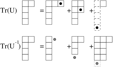
Figure 4: An example of the multiplication of the state $[2,1^{3}]$ in $SU(5)$ with $\operatorname{Tr}[U]$ and $\operatorname{Tr}[U^{-1}]$. This corresponds to the addition or subtraction of a square, such that a higher row is always larger than or equal to a lower one. A full column can be added or subtracted without changing the state. This is used to obtain a canonical form with the last column empty.

We can of course work directly in terms of the angular variables as discussed above. For some cases it is actually useful to consider $\operatorname{Tr}[U]$ and its complex conjugate as raising and lowering operators, which act in a simple way on the Young tableau labelling the symmetry of the wave function,

$$\operatorname{Tr}[U]\Phi_{[f]} = \sum_{i=0}^{N-1}\Phi_{[f_{1},\cdots,f_{i}+1,\cdots,f_{N-1},f_{N}]}\quad,$$

$$\operatorname{Tr}[U^{-1}]\Phi_{[f]} = \sum_{i=0}^{N-1}\Phi_{[f_{1},\cdots,f_{i}-1,\cdots,f_{N-1},f_{N}]}\quad,$$ (119)

where $f_{N}=0$ can be imposed, as discussed above. If at any stage in the calculation we end up with $f_{N}\not=0$, we can use Eq. (111) to make it zero. In summary, we need to use the three conditions

$$(f_{1},f_{2},\cdots,f_{N-1},-1) = (f_{1}+1,f_{2}+1,\cdots,f_{N-1}+1,0)\quad,$$

$$(n+f_{1},n+f_{2},\cdots,n+f_{N-1},n) = (f_{1},f_{2},\cdots,f_{N-1},0)\quad,$$

$$(f_{1},f_{2},\cdots,f_{i},\cdots,f_{i},\cdots,f_{N-1}) = 0\quad.$$ (120)

Even though this interpretation of the traces is quite appealing, it is not totally straightforward to use, since there is no cyclic vector; when acting on the state labelled by

$$[f]=[0^{N-1}]\quad,$$ (121)

both terms lead to non-vanishing results. This is intimately related to the existence of both covariant and contravariant representations of $SU(N)$ occurring at the same kinetic energy, which are mixed by the magnetic terms. An example is shown in Fig. 4.

5.3 The harmonic approximation

In the weak-coupling limit we can make the harmonic approximation, where we approximate the magnetic potential by its quadratic expansion, and we can ignore the periodicity of the $\psi$ variables since they oscillate near their equilibrium values. The resulting potential,

$$V(\{\psi\}) = {\lambda}\sum_{i=1}^{N}(\psi_{i}-\Psi)^{2}$$ (122)

$$= {\lambda}\left(\sum_{i=1}^{N}\psi^{2}-N\Psi^{2}\right)\quad,$$

is modified by confining the centre-of-mass in the harmonic oscillator (HO) potential $V(\Psi)=\frac{\lambda}{2}N\Psi^{2}$. We have reconstructed here the well-known separability of the many-body harmonic oscillator Hamiltonian into a centre-of-mass (CM) and relative part, where the CM part is in a harmonic oscillator state with frequency $N$ times larger (since the mass for the CM mode is also $N$ times the single-particle mass) than the single particle one (and see, e.g., Ref. [41]).

Amongst the spectrum of the $N$-fermion HO problem we have states with the CM in the $m=0,1,2,\ldots$ states, and we thus reproduce each relative state with all of the CM states. If we can determine all those states with the CM in its ground state, we immediately know the degeneracy of the $SU(N)$ spectrum. So we need to identify those states from amongst the degenerate multiplet with energy $(n+N/2)\hbar\omega$. Let $\nu_{n}$ be the degeneracy of this ($n$-th excited) energy level, which is given by the number of distinct partitions of $n$ into $N$ positive numbers:

$$\nu_{n}^{U(N)}=P_{N}(n)=\sum_{\lambda_{1}>\lambda_{2}>\cdots>\lambda_{N}\geq 0;\sum\lambda_{i}=n}1\quad.$$ (123)

We use the fact that harmonic oscillator wave functions are exponentials times a polynomial. Clearly the centre-of-mass polynomial can only arise from a linear combination of the polynomial parts of the various degenerate wave functions. For a CM ground state this polynomial part is a constant, and thus lies in the null space of the centre-of-mass momentum operator

$$P=\sum_{i=1}^{N}i\frac{\partial}{\partial\psi_{i}}\quad.$$ (124)

This operator maps the $n$-th degree polynomials onto the $(n-1)$-th degree polynomials. The dimension of the null space is the difference between the dimensions of the domain and range of the operator $P$. Therefore the degeneracy of the $n$-th relative motion, i.e., $SU(N)$, eigenstate is given by

$$\nu_{n}^{SU(N)}=P_{N}(n)-P_{N}(n-1)\quad.$$ (125)

For $N=2$

$$P_{2}(n)=\left[\frac{n+1}{2}\right]\quad,$$ (126)

where $[\ \cdot\ ]$ denotes the integer part of a number, and thus $\nu_{n}=\delta_{n,\text{odd}}$, which corresponds to a set of non-degenerate, odd wave functions for $SU(2)$. For $SU(3)$, $SU(4)$, and $SU(5)$ we find the degeneracies (the first state always occurs at $i=N(N-1)/2$, since all lower energy functions are not antisymmetric),

$$\{P_{3}(i)\}_{i=3}^{\infty} = \{1,1,2,3,4,5,7,8,10,12,14,\cdots\}\quad,$$

$$\{\nu_{i}^{SU(3)}\}_{i=3}^{\infty} = \{1,0,1,1,1,1,2,1,2,2,2,\cdots\}\quad,$$

$$\{P_{4}(i)\}_{i=6}^{\infty} = \{1,1,2,3,5,6,9,11,15,18,\cdots\}\quad,$$

$$\{\nu_{i}^{SU(4)}\}_{i=6}^{\infty} = \{1,0,1,1,2,1,3,2,4,3\cdots\}\quad,$$

$$\{P_{5}(i)\}_{i=10}^{\infty} = \{1,1,2,3,5,7,10,13,18,23,30,\cdots\}\quad,$$

$$\{\nu_{i}^{SU(5)}\}_{i=10}^{\infty} = \{1,0,1,1,2,2,3,3,5,5,7,\cdots\}\quad.$$ (127)

Notice the absence of the first excited state; $\nu_{N(N-1)/2+1}^{SU(N)}=0$, since the only state at that position is a centre-of-mass excitation built on the ground state. Note that our result differs from the result in Ref. [42], where the fact that only even functions in the radial coordinate are allowed was ignored. The $SU(3)$ spectrum is

$$\frac{2a}{g^{2}}E_{x}\sim 2\sqrt{2}\frac{1}{g^{2}}(3k+2n)\quad,$$ (128)

for $n=0,1,2,3,\ldots$ and $k=1,2,3,\ldots$.

5.4 Large-$N$ limit

The large-$N$ limit of QCD is one of the intriguing open problems in the theory, and one might wonder whether our result can shed some light on the much less taxing problem of the large-$N$ limit of the one-plaquette problem. In that case we have to study the Hamiltonian

$$H={2}\sum_{i}p_{i}^{2}+2\lambda\sum_{i=1}^{N}(1-\cos(\psi_{i}-\Psi))\quad.$$ (129)

The leading term is simply obtained from the Hartree-Fock approximation, with Hartree Hamiltonian

$$\mathcal{H}={2}p^{2}+2\lambda(1-\cos\psi)\quad,$$ (130)

and we can (if we wish) evaluate the Hartree-Fock energy for this state using the solutions of the Mathieu equation. The boundary conditions are strict periodicity, since the all the circles parametrised by $\psi_{i}$ are connected, and end up at the same physical point.

Such results are well-known from many-body theory [43]. In principle the next order in $1/N$ would follow from an RPA calculation. However, there are some problems. The interaction is explicitly $N$-dependent, since $\Psi$ depends on $N$, and the residual interaction is rather cumbersome to deal with.

5.5 Explicit solutions

Figure 5: Examples of the action of $\operatorname{Tr}U$ (solid lines with arrows) and $\operatorname{Tr}[U^{\dagger}]$ (dashed lines with arrows) on the states of $SU(3)$, labelled by the partition $[f_{1},f_{2}]$.

Let us now investigate the spectra of a few of the relevant gauge theories. The method we use to solve the problem is to work in a basis of eigenstates of the electric Hamiltonian, and evaluate the action of $\operatorname{Tr}U$ and $\operatorname{Tr}U^{\dagger}$ on these states. As can be seen from the example for $SU(3)$ shown in Fig. 5, there are several different coupling mechanisms. Nonetheless, this method is straightforward to implement, and leads to fully converged results up to large values of the effective coupling constant $1/g^{4}$.

5.5.1 The $U(1)$ one-plaquette problem

Figure 6: The lower end of the fully converged $U(1)$ one-plaquette spectrum. The lines starting from $4n^{2}$ are the periodic solutions, and the lines starting from $(2n+1)^{2}$ are anti-periodic ones. The hashed areas denote the existence of a continuum of Floquet states at these energies.

First we look at $U(1)$. This is something of a special case, as it does not fit into our general $SU(N)$ framework. However, the relation is straightforward. With the parametrisation $U=e^{i\phi}$, the electric operator is $i\partial/\partial\phi$. If we use the maximal tree formulation, we find that the action of the electric energy gets weighted by a factor of four, essentially one for each side of the plaquette. The magnetic part is $[2-\exp(i\phi)-\exp(-i\phi)]=2(1-\cos\phi)$, and hence the Schrödinger equation becomes

$$\frac{g^{2}}{2a}\left[-4\frac{d^{2}}{d\phi^{2}}+\frac{2}{g^{4}}(1-\cos\phi)\right]\Psi=E\Psi\quad.$$ (131)

Upon substitution of $2z=\phi$, $\alpha=2(Ea-1)/g^{2}$, $q=-2/g^{2}$, we find the Mathieu equation,

$$\frac{d^{2}y(z)}{dz^{2}}+(\alpha-2q\cos 2z)y(z)=0\quad.$$ (132)

However, we still need to analyse the boundary conditions on $\Psi$. It is well known from Floquet theory [44] that solutions of a differential equation with periodic coefficients are quasi-periodic,

$$\Psi_{\nu}=e^{i\pi\nu}\Psi\quad,$$ (133)

where $\Psi(\phi)=\Psi(\phi+\pi)$, and $\nu$ is a, in principle complex, exponent. The only normalisable solutions are those with a real exponent, and those are found bracketed between the (periodic) $\operatorname{ce}_{r}(z,q)$ and the $\operatorname{se}_{r+1}(z,q)$ solutions [45], as in Fig. 6. These results are analogous to the band structure in metals, due to the periodic potential in which the electrons move. We define a scaled energy $\varepsilon$ as

$$E=\frac{g^{2}}{2a}\varepsilon+\frac{N}{g^{2}a}\quad,$$ (134)

which we use for representing the numerical results.

For the period states we can attack the problem numerically by expanding the Hamiltonian in terms of the eigenstates, $\exp(in\phi)$, of the electric operator,

$$H_{\operatorname{ce}} = \sum_{n=0}|n\rangle\left(4\frac{n^{2}g^{2}}{2a}+\frac{1}{g^{2}a}\right)\langle n|\quad-\quad\frac{1}{2g^{2}a}\big{\{}|n\rangle\langle n+1|\quad+\quad|n+1\rangle(1+\delta_{0n})\langle n|\big{\}}$$ (135)

$$H_{\operatorname{se}} = \sum_{n=1}|n\rangle\left(4\frac{n^{2}g^{2}}{2a}+\frac{1}{g^{2}a}\right)\langle n|\quad-\quad\frac{1}{2g^{2}a}\big{\{}|n\rangle\langle n+1|\quad+\,\,|n+1\rangle\langle n|\big{\}}$$ (136)

where the sum starts at zero for $\operatorname{ce}_{2r}$ solutions and at one for $\operatorname{se}_{2r}$ solutions. This matrix equation serves as a relatively efficient way of determining the characteristic values $a$ and $b$ of the Mathieu equation, via straightforward numerical methods.

5.5.2 The $SU(2)$ one-plaquette problem

Figure 7: The lower end of the fully converged $SU(2)$ one-plaquette spectrum

The $SU(2)$ matrices have two complex conjugate eigenvalues, and can be parametrised as $\operatorname{Tr}(U)=2\cos\phi$, where $\phi=(\psi_{1}-\psi_{2})$, and see Eq. (92). If we absorb the factor $\Xi$ from Eq. (102) into the wave function ($\Xi=2\sin(\phi/2)$),

$$\Phi=\Xi\Psi$$ (137)

The Schrödinger equation, which takes the form

$$\frac{g^{2}}{2a}\left[-4\frac{\partial^{2}}{\partial\phi^{2}}-1+\frac{4}{g^{4}}(1-\cos(\phi/2))\right]\Phi=E\Phi\quad,$$ (138)

is again the Mathieu equation. In this case the interpretation is different, even though we still have $2z=\phi$, but $\phi$ plays a different role. As a function of the periodic quantity $\operatorname{Tr}U$, $\Phi$ must be strictly periodic. Due to the anti-symmetry induced by the Pauli principle, the only non-singular wave functions $\Psi$ are the odd Mathieu functions $\operatorname{se}_{1}(z,q),\operatorname{se}_{2}(z,q),\cdots$, for which $\alpha=b_{r}(q)$, where the index is allowed to take odd values, since the $2\pi$ periodicity on $[-\pi,\pi]$ is guaranteed by the solutions being odd. For $q=0$ the solutions reduce to $\Phi_{n}=\sin\frac{n+1}{2}\phi$, and since $\Xi\propto\sin\frac{1}{2}\phi$, $\Psi(-\pi)=\Psi(\pi)$. The solutions are shown in Fig. 7.

In terms of the eigenstates $|n\rangle$ of the electric operator the Hamiltonian reads

$$H=\sum_{n=0}|n\rangle\left(\frac{n(n+2)g^{2}}{2a}+\frac{2}{g^{2}a}\right)\langle n|\quad-\quad\frac{1}{g^{2}a}\big{\{}|n\rangle\langle n+1|\quad+\quad|n+1\rangle\langle n|\big{\}}\quad.$$ (139)

We see that the differences between the $U(1)$ case and the $SU(2)$ case lie in the diagonal part of the Hamiltonian, respectively $n^{2}$ and $(n+1)^{2}-1$, which result from the electric operator.

5.5.3 $SU(3)$ one-plaquette problem

Figure 8: The domains for $\phi_{1}$ and $\phi_{2}$, in the antisymmetric wavefunction $\Phi$.

The $SU(3)$ one-plaquette problem has two independent angular degrees of freedom. From the $U(3)$ parametrisation we see that these can be chosen as $\phi_{1}=\frac{1}{3}(2\psi_{1}-\psi_{2}-\psi_{3})$, $\phi_{2}=\frac{1}{3}(-\psi_{1}+2\psi_{2}-\psi_{3})$. The remaining combination, $\frac{1}{3}(-\psi_{1}-\psi_{2}+2\psi_{3})=-(\phi_{1}+\phi_{2})$, is linearly dependent.

The Hamiltonian in these angular coordinates becomes, using Eqs. (107) and (114),

$$\frac{g^{2}}{2a}\left[\frac{4}{3}\left\{-\frac{\partial^{2}}{\partial\phi_{1}^{2}}-\frac{\partial^{2}}{\partial\phi_{2}^{2}}+\frac{\partial^{2}}{\partial\phi_{1}\partial\phi_{2}}-3\right\}+\frac{1}{g^{4}}(3-\cos\phi_{1}-\cos\phi_{2}-\cos(\phi_{1}+\phi_{2}))\right]\Phi=E\Phi\quad,$$ (140)

where the boundary conditions are determined from the anti-symmetry of $\Psi$. The wave function vanishes if two eigenvalues of the matrix $U$ coincide, $\phi_{1}\not=\phi_{2}\not=-(\phi_{1}+\phi_{2})\not=\phi_{1}$. All variables are defined modulo $2\pi$, as they correspond to identical eigenvalues. We can restrict ourselves to the domain $-\phi_{1}-\phi_{2}\leq\phi_{1}$ , $\phi_{1}\leq\phi_{2}$, and $\phi_{2}\leq 2\pi-\phi_{1}-\phi_{2}$. However, many other choices of boundary conditions are possible, which follow from either permuting the variables, or translating the domain by $2\pi$. The $\phi_{1}\otimes\phi_{2}$ plane is divided into copies of the fundamental domain by the lines $\phi_{1}-\phi_{2}=n_{1}\pi$, $\phi_{1}+\frac{1}{2}\phi_{2}=n_{2}\pi$, and $\frac{1}{2}\phi_{1}+\phi_{2}=n_{3}\pi$, where $n_{i}\in\cdots,-2,-1,0,1,2,\cdots$, as shown in Fig. 8.

The potential can be simplified to

$$1+\cos\phi_{1}+\cos\phi_{2}+\cos(\phi_{1}+\phi_{2})=4\cos\frac{\phi_{1}}{2}\cos\frac{\phi_{2}}{2}\cos\frac{\phi_{1}+\phi_{2}}{2}\quad.$$ (141)

The explicit angular Schrödinger equation is useful for the harmonic approximation in the weak-coupling limit, however, for the strong-coupling limit and the intermediate region in coupling constants, the Hamiltonian in terms of the electric-operator eigenstates $|f_{1},f_{2}\rangle$ is more useful

$$H = \sum_{0\leq f_{2}\leq f_{1}}|f_{1},f_{2}\rangle\left(\frac{4(f_{1}^{2}+f_{2}^{2}+3f_{1}-f_{1}f_{2})g^{2}}{6a}+\frac{3}{g^{2}a}\right)\langle f_{1},f_{2}|$$ (142)

$$-\frac{1}{2g^{2}a}\big{\{}|f_{1},f_{2}\rangle\langle f_{1},f_{2}+1|\quad+\quad|f_{1},f_{2}\rangle\langle f_{1}+1,f_{2}|$$

$$+|f_{1}+1,f_{2}\rangle\langle f_{1},f_{2}|\quad+\quad|f_{1},f_{2}+1\rangle\langle f_{1},f_{2}|$$

$$+|f_{1},f_{2}\rangle\langle f_{1}+1,f_{2}+1|\quad+\quad|f_{1}+1,f_{2}+1\rangle\langle f_{1},f_{2}|\big{\}}\quad,$$

where all the states $|f_{1},f_{2}\rangle$ where the condition $0\leq f_{2}\leq f_{1}$ does not hold, are identical to zero. This problem does not seem to have a closed-form analytical solution, and we have to resort to numerical methods to obtain the spectrum for arbitrary values of the coupling constant $g$, as in Fig. 9.

Figure 9: The lower end of the fully converged $SU(3)$ one-plaquette spectrum

5.5.4 Higher orders

Figure 10: The lower end of the fully converged $SU(4)$ one-plaquette spectrum

Figure 11: The lower end of the fully converged $SU(5)$ one-plaquette spectrum

We conclude this section by showing results for the gauge groups $SU(4)$ (Fig. 10) and $SU(5)$ (Fig. 11). The most interesting aspect of these results is the presence of (what appear to be) real level crossings, which could be a reflection of some hidden symmetry in the problem. It was verified that the distance at these crossings was equal to zero within the numerical accuracy.

The region of the coupling constant shown in Figs. 6–11 is insufficient to see convergence to the harmonic approximation (127). We have checked numerically, for $g^{-4}\geq 50$, that these results are correct.

6 Wave functionals

The results for the one-plaquette problem have more consequences for variational wave functionals than one might suspect. If the trace of the one-plaquette matrix is used, the wave functional is a function of the group characters only. The wave functional, which is the sum of of one-plaquette functions,

$$\langle\{\psi_{\alpha i}\}|\Sigma\rangle=\sum_{\mathrm{plaquettes}\,\,\alpha}F\left(\{\psi_{\alpha i}\}_{i=1}^{N-1}\right)\quad\,\,,$$ (143)

naturally leads to the sum of one-plaquette problems, leading to the energies which are the sum one-plaquette energies. However, the product wave functional

$$\langle\{\psi_{\alpha i}\}|\Pi\rangle=\prod_{\mathrm{plaquettes}\,\,\alpha}F\left(\{\psi_{\alpha i}\}_{i=1}^{N-1}\right)\quad\,\,,$$ (144)

also leads to the same result. Note that the exponentiated potential, $\exp\{\kappa H_{M}\}$, where $\kappa$ is a parameter to be determined by a variational calculation, as a simple ansatz for the correlated wave functional [46] is a particular choice in this class of wave functionals. The absence of correlations between nearest-neighbour plaquettes, generally present, follows from the symmetry in the angular variables,

$$\Psi_{\lambda}(\cdots\psi_{i}\cdots\psi_{j}\cdots)=\Psi_{\lambda}(\cdots\psi_{j}\cdots\psi_{i}\cdots)\quad,$$ (145)

where

$$F(\psi_{1}\cdots\psi_{N})=\sum_{\lambda}c_{\lambda}\Psi_{\lambda}(\psi_{1}\cdots\psi_{N})\quad.$$ (146)

Therefore the product term from the electric operator vanishes,

$$D_{N}\Psi_{\lambda}^{\prime}(\psi_{\alpha 1}\cdots\psi_{\alpha N})\Psi_{\lambda^{\prime}}^{\prime}(\psi_{\beta 1}\cdots\psi_{\beta N}) = \Psi_{\lambda^{\prime}}^{\prime}(\psi_{\beta 1}\cdots\psi_{\beta N})D_{N}\Psi_{\lambda}^{\prime}(\psi_{\alpha 1}\cdots\psi_{\alpha N})$$ (147)

$$+ \Psi_{\lambda}^{\prime}(\psi_{\alpha 1}\cdots\psi_{\alpha N})D_{N}\Psi_{\lambda^{\prime}}^{\prime}(\psi_{\beta 1}\cdots\psi_{\beta N})\quad\,\,,$$

where $\alpha$ and $\beta$ are plaquettes containing the link $l$, and $\Psi_{\lambda}^{\prime}=J\Psi_{\lambda}$. The differential operator $D_{N}$ contains both sets of angular operators $\partial_{\psi_{i}}=\partial_{\psi_{\alpha i}}+\partial_{\psi_{\beta i}}$. Therefore the Hamiltonian, acting on the product wave functional $|\Pi\rangle$ also reduces to the sum of one-plaquette Hamiltonians.

7 Conclusions

With the understanding of both a gauge fixed Hamiltonian, and the one-plaquette problem we would now like to use this in a method designed to determine the ground-state wave function and excitations from the Hamiltonian. Since there are, in principle, an infinite number of degrees of freedom, some approximation is required. However, we want to do this in a systematic manner, where we can improve the order of approximation as required. The coupled cluster method (CCM) [35], a many-body technique, is suitable for such calculations. It has previously been applied lattice field theories, [47], and in various guises to gauge theory [48], although in a different context. It has also been applied to various spin-lattice problems in magnetism [49].

Central to the CCM is the parametrisation of the ket-state wave function as an exponential of excitation operators

$$|\Psi\rangle=e^{S}|\Phi\rangle\quad.$$ (148)

The bra-state contains the inverse exponential such that the Hamiltonian functional only contains linked terms of the excitation operators, due to the implicit similarity transform $e^{-S}He^{S}$. The projection on the model state $|\Phi\rangle$ is due to the annihilation operators $\tilde{S}$,

$$\langle\Psi| = \langle\Phi|(1+\tilde{S})e^{-S}\quad,$$

$$\langle\Psi| = \langle\Phi|e^{\tilde{S}}e^{-S}\quad,$$ (149)

where the first form is used in the normal coupled cluster method (NCCM), and the second form in the extended coupled cluster method (ECCM). The normal coupled cluster method does not reproduce the correct scaling limit when the excitation operators are obtained from the strong-coupling expansion.

However, this and the extreme difficulty of implementing the ECCM are related to the functional implementation of the CCM, where an operator is simply chosen to be the multiplication of the wave function with a function. We will only consider the operatorial CCM, where the creation operators excite from the model state to any arbitrary state, and do not act between different excited states on overlapping lattice-site configurations

$$S=\sum_{I}c_{I}|I\rangle\langle\Phi|\quad.$$ (150)

This allows us to implement the ECCM, which is better at describing a system at large global changes away from the model state $\Phi$.

The central question is the form of the states $|I\rangle$ in which to expand the Hilbert space. This is the question discussed in the first part of this paper. For the colourless sector we have to use closed contours, which are traces over products of $X$ variables, since only these variables are invariant under gauge transformations generated by Gauss’ law. The traces over $X$ variables are automatically closed contours as each contour associated with an $X$ variable starts and ends at the origin.

Our Hamiltonian is different from the naive Kogut-Susskind Hamiltonian used in Refs. [32, 31, 50], and this should have an important effect on the results we hope to obtain in our future work. The price we have to pay is that our Hamiltonian has a preferred direction, and we have lost explicit translational invariance. It is probably worthwhile to investigate different, more symmetrical, choices of the maximal tree. It would seem that the current choice should be very good to consider the interaction between fixed sources, which clearly break translational symmetry, but it is less obviously optimal for a study of the vacuum.

Appendix A One-dimensional many-fermion systems and their representations

As the ${SU}(N)$ one-plaquette problem can be mapped onto a one-dimensional $(N-1)$-fermion problem, we analyse the fermion problem in some depth to determine the spectrum and the action of a potential in coordinate representation. Usually fermion problems are dealt with in operator form, here we use the knowledge of (anti)symmetric functions to formulate the problem.

An $n$-fermion wave function is in terms of single-particle orbitals $\phi_{i}(x)$ given by the fully anti-symmetrised Slater determinant

$$\langle x_{1},\ldots,x_{N}|\Psi\rangle=\begin{vmatrix}\phi_{1}(x_{1})&\phi_{2}(x_{1})&\phi_{3}(x_{1})&\cdots&\phi_{n}(x_{1})\\ \phi_{1}(x_{2})&\phi_{2}(x_{2})&\phi_{3}(x_{2})&\cdots&\phi_{n}(x_{2})\\ \vdots&\vdots&\vdots&\cdots&\vdots\\ \phi_{1}(x_{n})&\phi_{2}(x_{n})&\phi_{3}(x_{n})&\cdots&\phi_{n}(x_{n})\end{vmatrix}\quad.$$ (151)

If $\phi_{m}(x)\equiv w(x)P_{m}(x)$ are chosen to be the lowest set of single-particle orbitals, in which $w$ is the weight function, which is the square root of the integration measure, and $P_{m}$ is the $m$-th orthogonal polynomial given that weight, then the wave function $\Psi$ is the ground state wave function $\Phi_{0}$. Only the linearly independent parts of each column in the Slater determinant contribute, and these are just the highest powers in each polynomial $P_{m}(x)\rightarrow x^{m}$. Therefore the ground-state Slater determinant reduces to the Vandermonde determinant

$$\langle x|\Phi_{0}\rangle=\frac{1}{\sqrt{n!}}\prod_{i=1}^{n}w(x_{i})\prod_{k<l}^{n}(x_{k}-x_{l})\quad.$$ (152)

As examples we deal with the infinite square well $[-\pi/2,\pi/2]$ and the harmonic oscillator. The one-particle wave functions are given, respectively, by

$$\{\phi\}_{\mathrm{s}.\mathrm{w}.} = \frac{2}{\sqrt{\pi}}\sin 2nx;\quad\frac{2}{\sqrt{\pi}}\cos(2n+1)x\quad,$$ (153)

$$\{\phi\}_{\mathrm{h}.\mathrm{o}.} = \frac{1}{\sqrt{2^{n}n!\sqrt{\pi}}}\mathrm{e}^{-x^{2}/2}H_{n}(x)\quad.$$ (154)

The sines and cosines can be re-expressed as polynomials in $\sin x$ with the weight $\cos x$. The infinite domain of the harmonic oscillator is of no consequence as the weight damps the wave function at large distances. The non-interacting $n$-fermion ground state consists of fermions in the lowest $n$ levels. We find

$$\langle x|\Phi_{0}\rangle_{\mathrm{s}.\mathrm{w}.} = \left(\frac{2}{\pi}\right)^{n/2}\frac{2^{[n/2]}[n/2]!}{\sqrt{n!}}\prod_{i=1}^{n}\cos x_{i}\prod_{k<l}^{n}(\sin x_{k}-\sin x_{l})\quad,$$ (155)

$$\langle x|\Phi_{0}\rangle_{\mathrm{h}.\mathrm{o}.} = \frac{1}{\pi^{n/4}}\left(\prod_{j=1}^{n-1}\sqrt{2^{j}j!}\right)^{-1}\frac{1}{\sqrt{n!}}\prod_{i=1}^{n}\mathrm{e}^{-x_{i}^{2}/2}\prod_{k<l}2(x_{k}-x_{l})\quad,$$ (156)

where the normalisation of the square-well wave function follows from De Moivre’s formula, and the normalisation of the harmonic oscillator wave function is a direct consequence of the normalisation of the Hermite polynomials $H_{n}$.

We now consider an arbitrary excited state $\Phi_{\lambda}$. Since the anti-symmetry is present by the ground-state wave function, the wave function of an excited state can be factorised as a symmetric function of all the variables times the ground-state wave function. For any finite basis, this symmetric function must be a symmetric polynomial

$$\langle x|\Phi_{\lambda}\rangle=S_{\lambda}(x)\langle x|\Phi_{0}\rangle\quad.$$ (157)

Now the possible excitations follow from the theory of symmetric polynomials, and can be labelled as a distinct partition $\lambda=(\lambda_{1},\lambda_{2}\,\cdots,\lambda_{n})$, where $\lambda_{i}$ is the label of an occupied level, in ascending order.

The symmetric polynomials are usually labelled independently of the degree of filling $n$ by the non-distinct partition $f=\lambda-\delta$ where $\delta=(n,n-1,\cdots,2,1)$ such that $f_{i}\leq f_{j}$ for $i>j$. The non-distinct partition $f$ yields the excitation with respect to the Fermi level (see Fig. 12).

Figure 12: The labelling of excitations in a fermionic system as non-distinct partitions, where any partition $\lambda_{1}\lambda_{2}\cdots$ for which $\lambda_{i}\geq\lambda_{j}$ if $i<j$ represents a unique excited state $|n(n-1)(n-2)\cdots\rangle\rightarrow|(n+\lambda_{1})(n-1+\lambda_{2})(n-2+\lambda_{3})\cdots\rangle$, where the labelling of states is the distinct partition.

Generally, the symmetric functions $S_{\lambda}$ are not of a definite degree and they have a normalisation that depends on $n$. So $\lambda$ refers to the leading order polynomial $S_{\lambda}=cs_{\lambda}+\cdots$. These polynomials $s_{\lambda}$ are the Schur functions [51],

$$s_{1} = \sum_{i}x_{i}\quad,$$

$$s_{2} = \sum_{i}x_{i}^{2}+\sum_{i<j}x_{i}x_{j}\quad,$$

$$s_{1,1} = \sum_{i<j}x_{i}x_{j}$$

$$s_{3} = \sum_{i}x_{i}^{3}+\sum_{i<j}(x_{i}^{2}x_{j}+x_{j}^{2}x_{i})+\sum_{i<j<k}x_{i}x_{j}x_{k}\quad,$$

$$s_{2,1} = \sum_{i<j}(x_{i}^{2}x_{j}+x_{j}^{2}x_{i})+2\sum_{i<j<k}x_{i}x_{j}x_{k}\quad,$$

$$s_{1,1,1} = \sum_{i<j<k}x_{i}x_{j}x_{k}\quad.$$ (158)

For ${SU}(N)$ one-plaquette problem the excited states are symmetric polynomials in the eigenvalues of the matrix $U\in{SU}(N)$. These polynomials are the Schur functions, $S_{\lambda}=s_{\lambda}$, and, as the eigenvalues lie on the complex unit circle, the symmetric polynomials are properly normalised. The eigenvalues of the electric operator follow directly from the definition. The two remaining problems are the action of the magnetic term on these states and how, and if, to express the symmetric polynomials, in the eigenvalues, again in terms of trace variables. For this purpose we introduce three representations: the Schur functions $s$, the monomial symmetric functions $m$, and the so-called trace functions $t$,

$$s_{\lambda} = \frac{\det x_{j}^{i-1+\lambda_{N-i+1}}}{\det x_{j}^{i-1}}\quad,$$

$$m_{\lambda} = \sum_{\mathrm{Perm}(i_{j})}x^{\lambda_{1}}_{i_{1}}x^{\lambda_{2}}_{i_{2}}\cdots x^{\lambda_{r}}_{i_{r}}\quad,$$

$$t_{\alpha} = \prod_{k}\left(\sum_{j}x_{j}^{k}\right)^{\alpha_{k}}\quad.$$ (159)

The numbers $\lambda$ denote a partition, and the $\alpha$ label can be related to a partition by

$$\lambda=(n^{\alpha_{n}}(n-1)^{\alpha_{n-1}}\cdots 2^{\alpha_{2}}1^{\alpha_{1}})\quad.$$ (160)

For instance, $\alpha=(1020\cdots 0)$ corresponds to $\lambda=(331)$.

From the relations between the different representations one can show that every excited state can be expressed as a product over traces. An excited state $s_{\lambda}$ of the ${SU}(N)$ one-plaquette problem is a partition of length less than $N$. If we use a lexicographical ordering $\succ$ [51], it means that $S_{\lambda}$ contains only monomials $m_{\kappa}$ where $\kappa\preceq\lambda$. It is easy to see that a trace function $t_{\nu}$ only contains monomials $m_{\kappa}$ where $\kappa\succeq\nu$. Therefore, an excited state $\Psi_{\lambda}$ from Eq. (90), can be expressed in terms of the $N-1$ independent trace variables, where

$$t_{\alpha_{1}\alpha_{2}\cdots\alpha_{N-1}}=\operatorname{Tr}[U]^{\alpha_{1}}\operatorname{Tr}[U^{2}]^{\alpha_{2}}\cdots\operatorname{Tr}[U^{N-1}]^{\alpha_{N-1}}\quad.$$ (161)

We can thus express the anti-symmetric wave functions in terms of the symmetric trace variables. One can easily construct the transition, or Kostka, tables [51] for transformations between $s$ and $m$, as well as $t$ and $m$.

Even though it is relatively straightforward to use trace variables for $SU(2)$, it turns out to be rather involved to extend these relations to higher-dimensional gauge theories. For example, with the relations above we can determine the integration measure for trace variables. For $SU(2)$ we require the relations up to the partitions of 4, while for $SU(3)$ we require similar relations for the partitions of 6,

$$SU(2):\quad\quad\Xi^{2} = 1-t_{1}^{2}\quad,$$ (162)

$$SU(3):\quad\quad\Xi^{2} = 27-5t_{1}^{3}+9t_{1}t_{2}-\frac{1}{2}t_{2}^{3}+\frac{5}{4}t_{1}^{2}t_{2}^{2}-t_{1}^{4}t_{2}+\frac{1}{4}t_{1}^{6}$$ (163)

$$= 27-18t_{1}t_{-1}+4(t_{1}^{3}+t_{-1}^{3})-t_{1}^{2}t_{-1}^{2}\quad.$$ (164)

where $t_{p}=\operatorname{Tr}[U^{p}]$. However, the use for this relation for $SU(3)$ is restricted as the two complex trace variables $t_{1}$ and $t_{2}$ have complicated relations, and are restricted to a non-trivial domain of the complex space ${\textbf{C}}^{2}$. Note that there are only two independent angular variables for $SU(3)$, which makes the angular variables much more useful than the trace variables.

The Haar measure $\mu(U)$ reduces to the measure of the trace variables if the integrand depends only on the trace variables,

$$\int d\mu(U)F(\{t_{\lambda}\})=\int\Xi dt_{1}\cdots dt_{N-1}F(\{t_{\lambda}\})=\int\Xi^{2}d\phi_{1}\cdots d\phi_{N-1}F(\{t_{\lambda}(\{\phi_{i}\})\})\quad,$$ (165)

where $\Xi$ is a non-polynomial function of the trace variables $t_{i}$.

A.1 The magnetic term

The magnetic terms in coordinate representation are just the multiplication of the state with $s_{1}$ and $s_{11\cdots 1}$, where $11\cdots 1$ is $1^{N-1}$. We can apply the Littlewood-Richardson rule for the general multiplication of two Schur functions,

$$s_{\lambda}s_{\kappa}=\sum_{\mu}c^{\mu}_{\lambda\kappa}s_{\mu}\quad.$$ (166)

However, since $s_{1}$ and $s_{11\cdots 1}$ are relatively simple we can derive multiplication rules from first principles, taking into account that the partitions cannot be longer than $N-1$. As symmetric polynomials we find ($x_{j}=\exp\{i\psi_{j}\}$),

$$\operatorname{Tr}[U] = x_{1}+x_{2}+x_{3}+\cdots+x_{N}\quad,$$ (167)

$$\operatorname{Tr}[U^{-1}] = x_{1}x_{2}\cdots x_{N-1}+\cdots+x_{1}x_{3}\cdots x_{N}+x_{2}x_{3}\cdots x_{N}\quad,$$ (168)

where we use that $x_{1}x_{2}\cdots x_{N}=1$. In terms of the partition $\lambda$ of $s_{\lambda}$, multiplying with $\operatorname{Tr}[U]$ means adding one to each in turn $\lambda_{i}\rightarrow\lambda_{i}+1$, cancelling all the partitions for which $\lambda_{i}>\lambda_{j}$ for $j<i$, due to the intrinsic anti-symmetry. Multiplying with $\operatorname{Tr}[U^{-1}]$ corresponds to $\lambda_{i}\rightarrow\lambda_{i}-1$, with the same cancellations.

This relation can be generalised to the multiplication by $\operatorname{Tr}[U^{p}]$ for any power $p$. This reduces to adding $p$ to each of the elements $\lambda_{i}$ in the partition $\lambda$. The partitions should be ordered $\lambda_{1}>\lambda_{2}>\cdots>\lambda_{N-1}>0$, and the non-distinct partitions dropped.

Appendix B Equivalent forms of the electric energy

In this section we prove that the electric operator in angular coordinates $\{\psi_{i}\}$,

$$D^{s}_{N}=-\frac{1}{2}\sum_{i=1}^{N}\frac{\partial^{2}}{\partial\psi_{i}^{2}}+\frac{1}{2}\left(\frac{1}{\sqrt{N}}\sum_{i=1}^{N}\frac{\partial}{\partial\psi_{i}}\right)^{2}\quad,$$ (169)

the $SU(N)$ equivalent of Eq. (107), Can be realised in the trace representation $\{\operatorname{Tr}[U^{p}]\}$ by the $SU(N)$ version of the electric operator in Eq. (90).

We start of by the relation between a function $F$ of the trace variables and one of the angular variables,

$$F\left(\operatorname{Tr}[U],\frac{1}{2}\operatorname{Tr}[U^{2}],\cdots,\frac{1}{N-1}\operatorname{Tr}[U^{N-1}]\right)=F\left(\sum_{i=1}^{N}e^{i\psi_{i}},\frac{1}{2}\sum_{i=1}^{N}e^{i2\psi_{i}},\cdots,\frac{1}{N-1}\sum_{i=1}^{N}e^{i(N-1)\psi_{i}}\right)\quad.$$ (170)

In order to prove the fundamental relation, we need to know the derivatives of the Vandermonde determinant with respect to the angular variables

$$\Delta_{j}=\frac{1}{\Delta}\frac{\partial}{\partial\psi_{j}}\Delta=\sum_{k\not=j}^{N}\frac{ie^{i\psi_{j}}}{e^{\psi_{j}}-e^{\psi_{k}}}\quad.$$ (171)

Writing out the terms in Eq. (107) we generate several terms,

$$\frac{1}{\Delta}D^{s}_{N}\Delta F=\boxed{\frac{1}{\Delta}[D^{s}_{N}\Delta]F}_{{\,\,I}}+\boxed{D^{s}_{N}F}_{{\,\,II}}-\boxed{\sum_{i=1}^{N}\Delta_{i}\partial_{i}F}_{{\,\,III}}+\boxed{\frac{1}{N}\left(\sum_{i=1}^{N}\Delta_{i}\right)\left(\sum_{i=1}^{N}\partial_{i}F\right)}_{{\,\,IV}}\quad,$$ (172)

where $\partial_{i}=\frac{\partial}{\partial\psi_{i}}$. Some tedious, but straightforward, calculations lead to

$$\mathrm{I} = \frac{N(N^{2}-1)}{24}F\quad,$$ (173)

$$\mathrm{II} = \frac{1}{2}\left(\sum_{p,q=1}^{N-1}\operatorname{Tr}[U^{p+q}]F_{,pq}+\sum_{p=1}^{N-1}p\operatorname{Tr}[U^{p}]F_{,p}\right)$$ (174)

$$- \frac{1}{2N}\left(\sum_{p,q=1}^{N-1}\operatorname{Tr}[U^{p}]\operatorname{Tr}[U^{q}]F_{,pq}+\sum_{p=1}^{N-1}p\operatorname{Tr}[U^{p}]F_{,p}\right)\quad,$$ (175)

$$\mathrm{III} = \frac{1}{2}\sum_{p=1}^{N-1}\left(\sum_{q=1}^{p-1}\frac{1}{2}\operatorname{Tr}[U^{p-q}]\operatorname{Tr}[U^{q}]+\left(N-\frac{1}{2}-\frac{p}{2}\right)\operatorname{Tr}[U^{p}]\right)F_{,p}\quad,$$ (176)

$$\mathrm{IV} = -\frac{N-1}{2}\sum_{p=1}^{N-1}\operatorname{Tr}[U^{p}]F_{,p}\quad,$$ (177)

which, when substituted back in the original equation, yields the $SU(N)$ version of Eq. (90):

$$E^{2}_{l}F\left(\left\{\frac{1}{p}{\rm Tr}[U^{p}]\right\}_{p}\right) = \sum_{p,q}\left(\frac{1}{2}{\rm Tr}[U^{p}U^{q}]-\frac{1}{2N}{\rm Tr}[U^{p}]{\rm Tr}[U^{q}]\right)F_{,pq}$$ (178)

$$+ \sum_{p}\left(\frac{N^{2}-p}{2N}{\rm Tr}[U^{p}]+\frac{1}{2}\sum_{q=1}^{p-1}{\rm Tr}[U^{p-q}]{\rm Tr}[U^{q}]\right)F_{,p}\ \ .$$ (179)

This finishes the proof.

References

• [1] C. N. Yang and R. L. Mills, Phys. Rev. 96 (1954), 191.
• [2] L. D. Faddeev and A. A. Slavnov, “Gauge Fields, Introduction to Quantum Theory,” Benjamin Cummings, Reading (Mass.), 1980.
• [3] P. A. M. Dirac, “Principles of Quantum Mechanics, ” 4th edition, Oxford University Press, Oxford, 1967.
• [4] P. A. M. Dirac, “Lectures on Quantum Mechanics,” Belfer Graduate School of Science (Yeshiva University), New York, 1964; P. A. M. Dirac, “Lectures on Quantum Field Theory,” Belfer Graduate School of Science (Yeshiva University), New York, 1966.
• [5] T. Muta, “Foundations of Quantum Chromodynamics,” World Scientific, Singapore, 1987.
• [6] M. Henneaux and C. Teitelboim, “Quantization of Gauge Systems,” Princeton University Press, Princeton, 1992.
• [7] J. Kogut and L. Susskind, Phys. Rev. D 11 (1975), 395.
• [8] J. B. Kogut, Rev. Mod. Phys. 51 (1979), 659.
• [9] F. A. Berezin, “The Method of Second Quantization,” Academic Press, New York, 1966.
• [10] B. Felsager, “Geometry, Particles and Fields,” Odense University Press, Odense, 1981.
• [11] G. ’t Hooft and M. Veltman, Nucl. Phys. B 44 (1972), 189.
• [12] K. Wilson, Phys. Rev. 179 (1969), 499.
• [13] I. Montvay and G. Münster, “Quantum Fields on a Lattice,” Cambridge Univ. Press, Cambridge, 1994.
• [14] B. E. Baaquie, Phys. Rev. D 32 (1985), 2774; Phys. Rev. D 33 (1986), 2367.
• [15] D. Stoll, Phys. Lett. B 336 (1994), 524.
• [16] R. W. Haymaker, preprint hep-lat/9809094.
• [17] N. H. Christ and T. D. Lee, Phys. Rev. D 22 (1980), 939.
• [18] V. F. Müller and W. Rühl, Nucl. Phys. B 230 (1984), 49.
• [19] J. B. Bronzan, Phys. Rev. D 31 (1985), 2020.
• [20] J. B. Bronzan, Phys. Rev. D 37 (1988), 1621.
• [21] J. B. Bronzan, Phys. Rev. D 38 (1988), 1994.
• [22] J. B. Bronzan and T. E. Vaughan, Phys. Rev. D 43 (1991), 3499.
• [23] J. B. Bronzan and T. E. Vaughan, Phys. Rev. D 47 (1993), 3543.
• [24] S. Mandelstam, Phys. Rev. D 19 (1979), 2391.
• [25] F. Lenz, H. W. L. Naus, and M. Thies, Ann. Phys. (N.Y.) 233 (1994), 317.
• [26] N. J. Watson, Phys. Lett. B 323 (1994), 385.
• [27] D. Horn and M. Karliner, Nucl. Phys. B 235 (1984), 135.
• [28] M. A. B. Bég and H. Ruegg, J. Math. Phys. 6 (1965), 677.
• [29] M. Creutz, J. Math. Phys. 19 (1974), 2043.
• [30] M. Creutz, “Quarks, Gluons, and Lattices,” Cambridge Univ. Press, Cambridge, 1983.
• [31] C. R. Leonard, Ph.D. thesis, Melbourne University, 1998.
• [32] D. Schütte, Zheng Weihong, and C. J. Hamer, Phys. Rev. D 55 (1997), 2974.
• [33] C. Di Bartolo, R. Gambini, and L. Leal, Phys. Rev. D 39 (1989), 1756.
• [34] W. Magnus, F. Oberhettinger, and R. P. Soni, “Formulas and Theorems for the Special Functions of Mathematical Physics,” Springer, Berlin, 1966.
• [35] R. F. Bishop, Theor. Chim. Acta 80 (1991), 95; in “Microscopic Quantum Many-Body Theories and Their Application,” J. Navarro and A. Polls (eds.), Lec. Notes in Physics 510, Springer, Berlin, 1998, p. 1.
• [36] J. E. Hetrick, Int. J. Mod. Phys. A9 (1994), 3153.
• [37] J. Hallin, Class. Quant. Grav. 11 (1994), 1615.
• [38] H. Weyl, “The Classical Groups,” 2nd edition, Princeton University Press, Princeton, 1946.
• [39] J. A. Minahan and A. P. Polychronakos, Phys. Lett. B 312 (1993), 155; Phys. Lett. B 326 (1994), 288; Interacting Fermion Systems from Two-Dimensional QCD, CERN preprint, 1993 ; M. R. Douglas, hep-th/9311130; Nucl. Phys. Proc. Suppl. 41 (1995), 66; M. Caselle, A. D’Adda, L. Magnea, and S. Panzeri, Nucl. Phys. B 416 (1994), 751.
• [40] P. Ring and P. Schuck, “The Nuclear Many-Body Problem,” Springer, New York, 1980.
• [41] M. Moshinski and Y. F. Smi, “The Harmonic Oscillator in Modern Physics ,” Harwood Academic, Amsterdam, 1996, (Contemporary concepts in physics, Vol. 9).
• [42] D. Robson and D. M. Webber, Z. Phys. C 7 (1980), 53.
• [43] J. P. Blaizot and G. Ripka, “Quantum Theory of Finite Systems,” MIT Press, Cambridge (Mass.), 1986.
• [44] E. T. Whittaker and G. N. Watson, “A Course in Modern Analysis,” Cambridge Press, Cambridge, 1927.
• [45] M. Abramowitz and I. A. Stegun, “Handbook of Mathematical Functions,” National Bureau of Standards, Dover, New York, 1965.
• [46] J. Greensite, Phys. Lett. B 191 (1987), 431.
• [47] N. E. Ligterink, N. R. Walet, and R. F. Bishop, Ann. Phys. (N.Y.) 267 (1998), 97.
• [48] S. J. Baker, R. F. Bishop, and N. J. Davidson, Phys. Rev. D 53 (1996), 2610; S. J. Baker, R. F. Bishop, and N. J. Davidson, Nucl. Phys. B (Proc. Supp.) 53 (1997), 834.
• [49] R. F. Bishop, J. B. Parkinson, and Yang Xian, Phys. Rev. B 44 (1991), 9425; D. J. J. Farnell, R. F. Bishop, and Chen, Zheng, J. Stat. Phys. 90 (1998) 327; J. Rosenfeld, N. E. Ligterink, and R. F. Bishop, Phys. Rev. B 60 (1999), 4030.
• [50] S.-H. Guo and X.-Q. Luo, preprint hep-lat/9706017.
• [51] I. G. MacDonald, “Symmetric Polynomials and Hall Functions,” Clarendon Press, Oxford, 1979.