Calibration of Smearing and Cooling Algorithms in SU(3)-Color Gauge Theory

Abstract

The action and topological charge are used to determine the relative rates of standard cooling and smearing algorithms in pure SU(3)-color gauge theory. We consider representative gauge field configurations on $16^{3}\times 32$ lattices at $\beta=5.70$ and $24^{3}\times 36$ lattices at $\beta=6.00$. We find the relative rate of variation in the action and topological charge under various algorithms may be succinctly described in terms of simple formulae. The results are in accord with recent suggestions from fat-link perturbation theory.

I Introduction

Cooling [1] is a well established method for locally suppressing quantum fluctuations in gauge field configurations. The locality of the method allows topologically nontrivial field configurations to survive numerous iterations of the cooling algorithm. Application of such algorithms are central to removing short-distance fluctuations responsible for causing renormalization constants to significantly deviate from one as is the case for the topological charge operator [2].

An alternative yet somewhat related approach is the application of APE smearing [3] to the gauge field configurations. Because the algorithm is applied simultaneously to all link variables, without any annealing in the process of a lattice update, the application of the algorithm may be viewed as an introduction of higher dimension irrelevant operators designed to improve the operator based on unsmeared links. This approach also leads to the desirable effect of renormalization constants approaching one. The net effect may be viewed as introducing a form factor to gluon vertices [4] that suppresses large $q^{2}$ interactions and, as a result, suppresses lattice artifacts at the scale of the cutoff.

The focus of this paper is to calibrate the relative rates of cooling and smearing as measured by the action and the topological charge. In doing so we aim to establish relationships between various algorithms and their internal parameters. It is well known that errors in the standard Wilson action eventually destroy (anti)instanton configurations and this effect is represented in the topological charge as sharp transitions from one integer to another. We find the timing analysis of these topological charge defects to be central to understanding the behavior of the various algorithms.

To bridge the gap between cooling and smearing and discover the origin of variations between these algorithms, we present a new algorithm for smearing the gauge fields which we refer to as Annealed $U$ Smearing or AUS smearing. In addition to comparing cooling and smearing, we also calibrate the effects of different smearing fractions, describing the balance between the unsmeared link and the smeared link.

There have been numerous studies of the dependence of vacuum matrix elements on the number of smoothing sweeps. Of particular note is the observation of cooling as a diffusive procedure [5], such that the distance $d$ affected by cooling is related to the square-root of the number of sweeps over the lattice, $n$. This random walk ansatz was further investigated by introducing the lattice spacing $a$, such that $d=a\sqrt{n}$ takes on a physical length [6]. With this simple formula, it is possible to effectively relate results from lattices of different $\beta$ ($a$) and different smoothing sweeps $n$. Extensive work on removing the dependence of particular quantities on the number of smoothing sweeps was carried out in Ref. [7]. There, highly improved actions are fine tuned to stabilize the instanton action and size under cooling. Moreover, a modification of the updating algorithm [8] allows one to define a physical length scale beyond which the physics is largely unaltered. Closer to the focus of this investigation, some exploratory comments favoring the possibility of calibrating under-relaxed cooling were made in Ref. [9]. We will lend further weight to this possibility in the following analysis.

This paper is divided as follows: Section II, briefly describes the gauge action and summarizes the numerical simulations examined in this study. Section III presents the relaxation algorithms and topological charge definition on the lattice. Sections IV A and  IV B present the numerical results for the action and topological charge trajectories respectively. A summary of our findings is provided in Section V.

II Lattice Gauge Action for $SU_{c}(3)$

A Gauge Action.

The Wilson action is defined as,

$$S_{G}=\beta\sum_{x}\sum_{\mu<\nu}\frac{1}{3}{\cal R}e\,{\rm Tr}(1-U_{\mu\nu}(x)),$$ (1)

where the operator $U_{\mu\nu}(x)$ is the standard plaquette,

$$U_{\mu\nu}(x)=U_{\mu}(x)\,U_{\nu}(x+\hat{\mu})\,U^{\dagger}_{\mu}(x+\hat{\nu})\,U^{\dagger}_{\nu}(x)\,.$$ (2)

Gauge configurations are generated using the Cabbibo-Marinari [10] pseudo–heat–bath algorithm with three diagonal $SU_{c}(2)$ subgroups. Simulations are performed using a parallel algorithm on a Thinking Machines Corporations (TMC) CM-5 with appropriate link partitioning. For the Wilson action we partition the link variables in the standard checkerboard fashion.

Configurations are generated on a $16^{3}\times{32}$ lattice at $\beta=5.70$ and a $24^{3}\times{36}$ lattice at $\beta=6.00$. Configurations are selected after 5000 thermalization sweeps from a cold start, and every 1000 sweeps thereafter. Lattice parameters are summarized in Table I. When required, we use the plaquette definition of the mean link variable.

TABLE I.: Parameters of the numerical simulations.

Action	Volume	$N_{\rm{Therm}}$	$N_{\rm{Samp}}$	$\beta$	$a$ (fm)	$u_{0}$	Physical Volume (fm)
Wilson	$16^{3}\times{32}$	5000	1000	5.70	0.18	0.86085	$2.88^{3}\times{5.76}$
Wilson	$24^{3}\times{36}$	5000	1000	6.00	0.10	0.87777	$2.4^{3}\times{3.6}$

III Cooling and Smearing Algorithms

Relaxation techniques have been the subject of a large amount of study in lattice QCD over the past few years [11]. Numerous algorithms have been employed to suppress the high-frequency components of the gauge field configurations in investigating their semi-classical content. In the following three subsections we consider three different algorithms that perform this task.

Perhaps it should be noted that cooling algorithms have been designed to render instantons stable over many hundreds of sweeps. For example, De Forcrand et al. [7] have established a five-loop improved gauge action that achieves this. However, our interest here is in using the defects in the topological charge evolution under standard cooling and smearing algorithms based on the Wilson gauge action to calibrate these algorithms.

A Cooling

Standard cooling minimizes the action locally at each link update. The preferred algorithm is based on the Cabbibo-Marinari [10] pseudo-heat-bath algorithm for constructing $SU_{c}(3)$-color gauge configurations. A brief summary of a link update follows.

At the $SU_{c}(2)$ level the algorithm is transparent. An element of $SU_{c}(2)$ may be parameterized as, $U=a_{0}I+i\,\vec{a}\cdot\vec{\sigma}$, where $a$ is real and $a^{2}=1$. Let $\widetilde{U}_{\mu}$ be one of the six staples associated with creating the plaquette associated with a link $U_{\mu}$.

$$\widetilde{U}_{\mu}=U_{\nu}(x+\hat{\mu})\,U^{\dagger}_{\mu}(x+\hat{\nu})\,U^{\dagger}_{\nu}(x)\,.$$ (3)

We define

$$\sum_{\alpha=1}^{6}\widetilde{U}_{\alpha}=k\overline{U} \hskip 15.6491pt{\rm where}\hskip 15.6491pt \overline{U}\in SU_{c}(2)\hskip 15.6491pt{\rm and}\hskip 15.6491ptk^{2}\equiv{\det\left(\sum_{\alpha=1}^{6}\widetilde{U}_{\alpha}\right)}\,.$$ (4)

The feature of the sum of ${SU_{c}(2)}$ elements being proportional to an ${SU_{c}(2)}$ element is central to the algorithm. The local ${SU_{c}(2)}$ action is proportional to

$${\cal R}e\,{\rm Tr}(1-U\overline{U})\,,$$ (5)

and is locally minimized when ${\cal R}e\,{\rm Tr}(U\overline{U})$ is maximized, i.e. when

$${\cal R}e\,{\rm Tr}(U\overline{U})={\cal R}e\,{\rm Tr}(I)\,.$$ (6)

which requires the link to be updated as

$$U{\longrightarrow}U^{\prime}=\overline{U}^{-1}=\overline{U}^{\dagger}=\frac{\left(\sum^{6}_{\alpha=1}\widetilde{U_{\alpha}}\right)^{\dagger}}{k}\,.$$ (7)

At the ${SU_{c}(3)}$ level, one successively applies this algorithm to various ${SU_{c}(2)}$ subgroups of ${SU_{c}(3)}$, with ${SU_{c}(2)}$ subgroups selected to cover the ${SU_{c}(3)}$ gauge group.

We explored cooling gauge field configurations using two diagonal $SU_{c}(2)$ subgroups. The cooling rate is slow and the action density is not smooth, even after 50 sweeps over the lattice. Addition of the third diagonal $SU_{c}(2)$ subgroup provides acceptably fast cooling and a smooth action density. These $SU_{c}(2)$ subgroups are acting as a covering group for the $SU_{c}(3)$ gauge group. One would therefore expect that repeated updates of $SU_{c}(2)$ subgroups will better approximate the ultimate ${SU_{c}(3)}$ link.

B Smearing

Here we consider two algorithms for smearing the gauge links. APE smearing [3] is now well established. Our alternate algorithm AUS smearing is designed to remove instabilities of the APE algorithm and provide an intermediate algorithm sharing features of both smearing and cooling.

1 APE Smearing

APE smearing [3] is a gauge equivariant [12] prescription for averaging a link $U_{\mu}(x)$ with its nearest neighbors $U_{\mu}(x+\hat{\nu}),\ \nu\neq\mu$. The linear combination takes the form:

$$U_{\mu}(x)\longrightarrow{U_{\mu}^{\prime}(x)}=(1-\alpha)U_{\mu}(x)+\frac{\alpha}{6}\widetilde{\Sigma}^{\dagger}(x;\mu),$$ (8)

where $\widetilde{\Sigma}(x;\mu)=\left(\sum^{6}_{\nu=1}\widetilde{U_{\nu}}(x)\right)_{\mu}$, is the sum of the six staples defined in Eq. (3). The parameter $\alpha$ represents the smearing fraction. The algorithm is constructed as follows: (i) calculate the staples, $\widetilde{\Sigma}(x;\mu)$; (ii) calculate the new link variable $U_{\mu}^{\prime}(x)$ given by Eq. (8) and then reunitarize $U_{\mu}^{\prime}(x)$; (iii) once we have performed these steps for every link, the smeared $U^{\prime}_{\mu}(x)$ are mapped into the original $U_{\mu}(x)$. This defines a single APE smearing sweep which can then be repeated.

The celebrated feature of APE smearing is that it can be realized as higher-dimension operators that might appear in a fermion action for example. Indeed, “fat link” actions based on the APE algorithm are excellent candidates for an efficient action with improved chiral properties [13]. The parameter space of fat link actions is described by the number of smearing sweeps $n_{\rm ape}$ and the smearing coefficient $\alpha$. It is the purpose of this investigation to explore the possible reduction of the dimension of this parameter space from two to one.

2 AUS Smearing

The Annealed $U$ Smearing (AUS) algorithm is similar to APE smearing in that we take a linear combination of the original link and the associated staples, $\widetilde{\Sigma}^{\dagger}(x;\mu)$. However in AUS smearing we take what was a single APE smearing sweep over all the links on the lattice and divide it up into four partial sweeps based on the direction of the links. One partial sweep corresponds to an update of all links oriented in one of the four Cartesian directions denoted $\mu=1,..,4$. Hence in a partial sweep we calculate the reuniterized $U_{\mu}^{\prime}(x)$ for all $\mu$–oriented links and update all of these links $[U_{\mu}^{\prime}(x)\longrightarrow{U_{\mu}(x)}]$ at the end of each partial sweep.

Thus the difference between AUS smearing and APE smearing is that in APE smearing no links are updated until all four partial sweeps are completed, while in AUS smearing, updated smeared information is cycled into the calculation of the next link direction, a process commonly referred to as annealing. In a sense AUS smearing is between cooling and APE smearing in that cooling updates one link at a time, AUS smearing updates one Cartesian direction at a time, and APE smearing updates the whole lattice at the same time.

As for APE smearing, the reunitarization of the $SU_{c}(3)$ matrix is done using the standard row by row orthonormalization procedure: begin by normalizing the first row; then update the second row by $row2=row2-(row2\cdot{row1})row1$; normalize the second row; finally set $row3$ equal to the cross product of $row1$ and $row2$.

For $SU_{c}(2)$ gauge theory, cooling and smearing are identical for the case of $\alpha=1$ when the links are updated one at a time. The AUS algorithm changes the level of annealing and provides the opportunity to alter the degree of smoothing. At the same time the AUS algorithm preserves the gauge equivariance of the APE algorithm for $SU_{c}(3)$ gauge theory [12]. As we shall see, it also removes the instability of the APE algorithm at large smearing fractions $\alpha$. This latter feature may provide a more efficient method for finding the fundamental modular region of Landau Gauge in trying to understand the effects of Gribov copies in gauge dependent quantities such as the gluon-propagator [14].

C Topological Charge

We construct the lattice topological charge density operator analogous to the standard Wilson action via the clover definition of ${F}_{\mu\nu}$. The topological charge $Q_{\rm{L}}$ and the topological charge density $q_{\rm{L}}(x)$ are defined as follows

$$Q_{\rm{L}}{\equiv}\sum_{x}{q_{\rm{L}}(x)}=\frac{g^{2}}{32\pi^{2}}\,\epsilon_{\mu\nu\rho\sigma}\,\sum_{x}\,{\rm Tr}({F}_{\mu\nu}(x)\,{F}_{\rho\sigma}(x))\,.$$ (9)

where the field strength tensor is

$$a^{2}\,g\,F_{\mu\nu}(x)=-\frac{i}{8}\left[\left({\cal O}_{\mu\nu}(x)-{\cal O}_{\mu\nu}^{\dagger}(x)\right)-\frac{1}{3}\,{\rm Tr}\left({\cal O}_{\mu\nu}(x)-{\cal O}_{\mu\nu}^{\dagger}(x)\right)\right]+{\cal O}(a^{4})\,,$$ (10)

and ${\cal O}_{\mu\nu}(x)$ is

$${\cal O}_{\mu\nu}(x) = U_{\mu}(x)\,U_{\nu}(x+\hat{\mu})\,U^{\dagger}_{\mu}(x+\hat{\nu})\,U^{\dagger}_{\nu}(x)$$ (11)

$$+ U_{\nu}(x)\,U^{\dagger}_{\mu}(x+\hat{\nu}-\hat{\mu})\,U^{\dagger}_{\nu}(x-\hat{\mu})\,U_{\mu}(x-\hat{\mu})$$ (12)

$$+ U_{\mu}(x-\hat{\mu})\,U^{\dagger}_{\nu}(x-\hat{\mu}-\hat{\nu})\,U_{\mu}(x-\hat{\mu}-\hat{\nu})\,U_{\nu}(x-\hat{\nu})$$ (13)

$$+ U^{\dagger}_{\nu}(x-\hat{\nu})\,U_{\mu}(x-\hat{\nu})\,U_{\nu}(x+\hat{\mu}-\hat{\nu})\,U^{\dagger}_{\mu}(x)\,.$$ (14)

Lattice operators possess a multiplicative lattice renormalization factor, $Q_{L}={\cal Z}_{Q}(\beta)\,Q$ which relates the lattice quantity $Q_{L}$ to the continuum quantity $Q$. Perturbative calculations indicate ${\cal Z}_{Q}(\beta)\approx 1-5.451/\beta+{\cal O}(1/{\beta^{2}})$ [2]. This large renormalization causes a problem when one is working at $\beta\approx 6.0$, as ${\cal Z}_{Q}(\beta)\ll{1}$. This implies that the topological charge is almost impossible to calculate directly. However when one applies cooling or smearing techniques to remove the problem of the short range quantum fluctuations giving rise to ${\cal Z}_{Q}(\beta)\ll{1}$, one can resolve near integer topological charge. One can apply the operator $Q_{L}$ to cooled configurations or smeared configurations. The latter case may be regarded as employing an improved operator in which the smeared links are understood to give rise to additional higher dimension irrelevant operators designed to provide a smooth approach to the continuum limit.

IV Numerical Simulations

We analyzed two sets of gauge field configurations generated using the Cabbibo-Marinari [10] pseudo-heat-bath algorithm with three diagonal $SU_{c}(2)$ subgroups as described in Table I. Analysis of a few configurations proves to be sufficient to resolve the nature of the algorithms in question. The two sets are composed of ten $16^{3}\times 32$ configurations and five $24^{3}\times 36$ configurations. For each configuration we separately performed 200 sweeps of cooling, 200 sweeps of APE smearing at four values of the smearing fraction and 200 sweeps of AUS smearing at six values of the smearing fraction.

For clarity, we define the number of times an algorithm is applied to the entire lattice as $n_{c}$, ${n_{\rm{ape}}(\alpha)}$ and $n_{\rm{aus}}(\alpha)$ for cooling, APE smearing and AUS smearing respectively. We monitor both the total action normalized to the single instanton action $S_{0}=8\pi^{2}/g^{2}$ and the topological charge $Q_{\rm{L}}(x)$ of Eq. (9) and observe their evolution as a function of the appropriate sweep variable and smearing fraction $\alpha$.

For APE smearing we consider four different values for the smearing fraction $\alpha$ including 0.30, 0.45, 0.55, and 0.70. Larger smearing fractions reveal an instability in the APE algorithm where the links are rendered to noise.

The origin of this instability is easily understood in fat-link perturbation theory [4] where the smeared vector potential after $n$ APE smearing steps is given by

$$A_{\mu}^{(n+1)}(q)=\sum_{\nu}\left[f^{n}(q)\,\left(\delta_{\mu\nu}-{\widehat{q}_{\mu}\widehat{q}_{\nu}\over\widehat{q}^{2}}\right)+{\widehat{q}_{\mu}\widehat{q}_{\nu}\over\widehat{q}^{2}}\right]A_{\nu}^{(n)}(q)\,,$$ (15)

reflecting the transverse nature of APE smearing. Here

$$\widehat{q}_{\mu}={2\over a}\sin\left({a\,q_{\mu}\over 2}\right)$$ (16)

and

$$f(q)=1-{\alpha\over 6}\,\widehat{q}^{2}\,.$$ (17)

For $f(q)$ to act as a form factor at each vertex in perturbation theory over the entire Brillouin zone

$$-{\pi\over a}<q_{\mu}\leq{\pi\over a}\,,$$ (18)

one requires $-1\leq f(q)\leq 1$ which constrains $\alpha$ to the range $0\leq\alpha\leq 3/4$.

The annealing process in AUS smearing removes this instability. Hence, the parameter set for AUS smearing consists of the APE set plus an extra two, $\alpha=0.85$ and 1.00.

A The Action Analysis.

1 APE and AUS Smearing Calibration

The action normalized to the single instanton action $S/S_{0}$ can provide some insight into the number of instantons left in the lattice as a function of the sweep variable for each algorithm. However, our main concern is the relative rate at which the algorithms perform. In Fig. 1, we show $S/S_{0}$ as a function of cooling sweep on the $24^{3}\times{36}$ lattice for five different configurations. The close proximity of the five curves is typical of the configuration dependence of the normalized action $S/S_{0}$.

FIG. 1.: The ratio $S/S_{0}$ as a function of cooling sweeps $n_{c}$ for five configurations on the $24^{3}\times{36}$ lattice at $\beta=6.00$. The single instanton action is $S_{0}=8\pi^{2}/g^{2}$.

Figures 2 and 3 report results for APE and AUS smearing respectively. Here we focus on one of the five configurations, noting that similar results are found for the other configurations. Each curve corresponds to a different value of the smearing fraction $\alpha$.

FIG. 2.: The ratio $S/S_{0}$ as a function of APE smearing sweeps $n_{\rm{ape}}(\alpha)$ for a configuration on a $24^{3}\times{36}$ lattice at $\beta=6.00$. Each curve has an associated smearing fraction $\alpha$.

FIG. 3.: The ratio $S/S_{0}$ as a function of AUS smearing sweep $n_{\rm{aus}}(\alpha)$ for a configuration on a $24^{3}\times{36}$ lattice at $\beta=6.00$. Each curve has an associated smearing fraction $\alpha$.

A similar analysis of the $16^{3}\times{32}$ lattice at $\beta=5.70$ is also performed yielding analogous results. In fact, taking the physical volumes of the two lattices into account reveals qualitatively similar action densities after 200 sweeps.

Note that in Fig. 3, the curve associated with the smearing parameter $\alpha=1.00$, crosses over the one generated at $\alpha=0.85$, when the sweep number, $n_{\rm{aus}}(\alpha)$, is approximately 40 sweeps. Thus $\alpha=1$ is not the most efficient smearing fraction for untouched gauge configurations. However, as the configurations become smooth, $\alpha=1.00$ becomes the most efficient.

To calibrate the rate at which the algorithms reduce the action, we record the number of sweeps $n(\alpha)$ required for the smeared action to cross various thresholds $S_{T}$. This is repeated for each of the smearing fractions $\alpha$ under consideration. In establishing the relative $\alpha$ dependence for the number of sweeps $n(\alpha)$, we first consider a simple linear relation between the number of sweeps required to cross $S_{T}$ at one $\alpha$ compared to another $\alpha^{\prime}$, i.e.

$$n(\alpha^{\prime})=c_{0}+c_{1}\,n(\alpha)\,.$$ (19)

Anticipating that $c_{0}$ will be small if not zero, we divide both sides of this equation by $n(\alpha)$ and plot as a function of $n(\alpha)$. Deviations from a horizontal line will indicate failings of our linear assumption.

Fig. 4 displays results for $\alpha^{\prime}$ fixed to 0.55 for the APE smearing algorithm and Fig. 5 displays analogous results for AUS smearing. We omit thresholds that result in $n(0.55)<10$ as these points will have integer discretization errors exceeding 10%. For $\alpha=0.70$ discretization errors the order of 10% are clearly visible in both figures.

FIG. 4.: The ratio $n_{\rm{ape}}(0.55)/n_{\rm{ape}}(\alpha)$ versus $n_{\rm{ape}}(\alpha)$ for numerous threshold actions on the $24^{3}\times{36}$ lattice at $\beta=6.00$. From top down the data points correspond to $\alpha=0.70$, 0.55, 0.45 and 0.30.

FIG. 5.: The ratio $n_{\rm{aus}}(0.55)/n_{\rm{aus}}(\alpha)$ versus $n_{\rm{aus}}(\alpha)$ for numerous threshold actions on the $24^{3}\times{36}$ lattice at $\beta=6.00$. From top down the data points correspond to $\alpha=1.00$, 0.85, 0.70, 0.55, 0.45, 0.30.

For the smearing fraction $\alpha\leq 0.85$ both plots show little dependence of $n(\alpha^{\prime}=0.55)/n(\alpha)$ on $n(\alpha)$. This supports our simple ansatz of Eq. (19) and indicates $c_{0}$ is indeed small as one would expect.

The non-linear behavior for $\alpha=1.00$ in AUS smearing, in Fig. 5, reflects the cross over in Fig. 3, for $\alpha=1.00$. For unsmeared configurations, $\alpha=1.00$ appears to be too large. Further study in $SU_{c}(2)$ is required to resolve whether the origin of the smearing inefficiency lies in the sum of staples lying too far outside the $SU_{c}(3)$ gauge group for useful reunitarization, or whether the annealing of the links in AUS smearing is insufficient relative to cooling.

To determine the $\alpha$ dependence of $c_{1}$, we plot $c_{1}=\langle n(\alpha^{\prime}=0.55)/n(\alpha)\rangle$ as a function of $\alpha$. Here the angular brackets denote averaging over all the threshold values considered; i.e. averaging over data in the horizontal lines of Figs. 4 and 5.

Fig. 6 for APE smearing and Fig. 7 for AUS smearing indicate the relationship between $c_{1}$ and $\alpha$ is linear with zero intercept to an excellent approximation. Indeed, ignoring the point at $\alpha=1$ for AUS smearing, one finds the same coefficients for the $\alpha$ dependence of APE and AUS smearing. When the fits are constrained to pass through the origin, one finds a slope of 1.818 which is the inverse of $\alpha^{\prime}=0.55$. Hence we reach the conclusion that

$$\frac{n_{\rm{ape}}(\alpha^{\prime})}{n_{\rm{ape}}(\alpha)}\simeq\frac{\alpha}{\alpha^{\prime}}\hskip 15.6491pt{\rm and}\hskip 15.6491pt\frac{n_{\rm{aus}}(\alpha^{\prime})}{n_{\rm{aus}}(\alpha)}\simeq\frac{\alpha}{\alpha^{\prime}}\,.$$ (20)

FIG. 6.: Illustration of the $\alpha$ dependence of $c_{1}=\langle n(\alpha^{\prime}=0.55)/n(\alpha)\rangle$ for APE smearing. The solid line fit to the data indicates $c_{1}=1.838\,\alpha-0.011$ whereas the dashed line, constrained to pass through the origin, provides a slope of 1.818.

FIG. 7.: Illustration of the $\alpha$ dependence of $c_{1}=\langle n(\alpha^{\prime}=0.55)/n(\alpha)\rangle$ for AUS smearing. Fits to the data exclude the point at $\alpha=1$. The solid line fit to the data indicates $c_{1}=1.857\,\alpha-0.021$ whereas the dashed line, constrained to pass through the origin, provides a slope of 1.818.

This analysis based on the action suggests that a preferred value for $\alpha$ does not really exist. In fact it has been recently suggested that one should anticipate some latitude in the values for $n(\alpha)$ and $\alpha$ that give rise to effective fat-link actions [4]. What we have done here is established a relationship between $n(\alpha)$ and $\alpha$, thus reducing what was potentially a two dimensional parameter space to a one dimensional space. This conclusion will be further supported by the topological charge analysis below.

To summarize these finding we plot the ratios

$$\frac{\alpha^{\prime}\,n_{\rm{ape}}(\alpha^{\prime})}{\alpha\,n_{\rm{ape}}(\alpha)}\hskip 15.6491pt{\rm and}\hskip 15.6491pt\frac{\alpha^{\prime}\,n_{\rm{aus}}(\alpha^{\prime})}{\alpha\,n_{\rm{aus}}(\alpha)}\,,$$ (21)

designed to equal 1 in Figs. 8 and 9 for APE and AUS smearing respectively. Figs. 10 and 11 report the final results of a similar analysis for APE and AUS smearing respectively at $\beta=5.7$. Here the $\alpha=1.0$ results are omitted from the AUS smearing results for clarity.

FIG. 8.: Illustration of the degree to which the relations of (20) are satisfied for the action under APE smearing. Here $\alpha<\alpha^{\prime}$ and $\alpha^{\prime}=0.30$, 0.45, 0.55, and 0.70. Data are from the $24^{3}\times{36}$ lattice at $\beta=6.0$.

FIG. 9.: Illustration of the degree to which the relations of (20) are satisfied for the action under AUS smearing. Here $\alpha<\alpha^{\prime}$ and $\alpha^{\prime}=0.30$, 0.45, 0.55, 0.70 and 0.85. Data are from the $24^{3}\times{36}$ lattice at $\beta=6.0$.

FIG. 10.: Illustration of the degree to which the relations of (20) are satisfied for the action under APE smearing. Here $\alpha<\alpha^{\prime}$ and $\alpha^{\prime}=0.30$, 0.45, 0.55, and 0.70. Data are from the $16^{3}\times{32}$ lattice at $\beta=5.7$.

FIG. 11.: Illustration of the degree to which the relations of (20) are satisfied for the action under AUS smearing. Here $\alpha<\alpha^{\prime}$ and $\alpha^{\prime}=0.30$, 0.45, 0.55, 0.70 and 0.85. Data are from the $16^{3}\times{32}$ lattice at $\beta=5.7$.

2 Cooling Calibration

Here we repeat the previous analysis, this time comparing cooling with APE and AUS smearing. We make the same linear ansatz for the relationship and plot $n_{c}/n_{\rm{ape}}(\alpha)$ versus $n_{\rm{ape}}(\alpha)$ for APE smearing in Fig. 12. Fig. 13 reports the ratio $n_{c}/n_{\rm{aus}}(\alpha)$ versus $n_{\rm{aus}}(\alpha)$ for AUS smearing. At small numbers of smearing sweeps, large integer discretization errors the order of 25% are present, as $n_{c}$ is as small as 4. With this in mind, we see an independence of the ratio on the amount of cooling/smearing over a wide range of smearing sweeps for both APE and AUS smearing. This supports a linear relation between the two algorithms.

FIG. 12.: Ratio of cooling to APE smearing sweeps as a function of the number of APE smearing sweeps. From top down $\alpha=0.70$ 0.55, 0.45 and 0.30.

FIG. 13.: Ratio of cooling to AUS smearing sweeps as a function of the number of AUS smearing sweeps. From top down $\alpha=1.00$, 0.85 0.70 0.55, 0.45 and 0.30.

Averaging the results provides

$$\frac{n_{c}}{n_{\rm{ape}}(0.55)}=0.330\hskip 15.6491pt{\rm and}\hskip 15.6491pt\frac{n_{c}}{n_{\rm{aus}}(0.55)}=0.340\,,$$ (22)

or more generally

$$n_{c}\simeq 0.600\,\alpha\,{n_{\rm{ape}}(\alpha)}\hskip 15.6491pt{\rm and}\hskip 15.6491ptn_{c}\simeq 0.618\,\alpha\,{n_{\rm{aus}}(\alpha)}\,.$$ (23)

Hence we see that cooling is much more efficient at smoothing than the smearing algorithms requiring roughly half the number of sweeps for a given product of $n$ and $\alpha$.

Equating the equations of Eq. (23) provides the following relation between APE and AUS smearing

$$\alpha\,{n_{\rm{ape}}(\alpha)}\simeq 1.03\,\alpha^{\prime}\,{n_{\rm{aus}}(\alpha^{\prime})}\,,$$ (24)

summarizing the near equivalence of the two smearing algorithms. It is important to recall that the annealing of the AUS smearing algorithm removes the instability of APE smearing encountered at large smearing fractions, $\alpha$. Thus AUS smearing offers a more stable gauge equivariant smoothing of gauge fields. It offers faster smoothing due to its ability to handle larger smearing fractions. This algorithm may be of use in studying Gribov ambiguities in Landau gauge fixing [12].

A similar analysis of the $16^{3}\times{32}$ lattice at $\beta=5.7$ provides

$$n_{c}\simeq 0.572\,\alpha\,{n_{\rm{ape}}(\alpha)}\hskip 15.6491pt{\rm and}\hskip 15.6491ptn_{c}\simeq 0.604\,\alpha\,{n_{\rm{aus}}(\alpha)}\,,$$ (25)

with

$$\alpha\,{n_{\rm{ape}}(\alpha)}\simeq 1.06\,\alpha^{\prime}\,{n_{\rm{aus}}(\alpha^{\prime})}\,.$$ (26)

Here the change in the coefficient relating APE smearing to cooling appears to be proportional to $\beta$.

B The Topological Charge Density Analysis.

Typical evolution curves for the lattice topological charge operator of Eq. (9) are shown in Figs. 14, 15 and 16 for APE smearing, AUS smearing and cooling respectively. These data are obtained from a typical gauge configuration on our $24^{3}\times{36}$ lattice at $\beta=6.00$. The configuration used here is the same representative configuration illustrated in Figs. 2 and 3 of the action analysis.

FIG. 14.: Typical evolution curve of the lattice topological charge operator as a function of the number of sweeps for APE smearing. Data are from the $24^{3}\times{36}$ lattice at $\beta=6.00$. Each curve corresponds to a particular $\alpha$ value and indicated.

FIG. 15.: Typical evolution curve of the lattice topological charge operator under AUS smearing. Data are from the $24^{3}\times{36}$ lattice at $\beta=6.00$. Each curve corresponds to a particular $\alpha$ value and indicated.

FIG. 16.: Typical evolution curve of the lattice topological charge operator as a function of the number of sweeps for cooling with three diagonal SU(2) subgroups on a $24^{3}\times{36}$ lattice at $\beta=6.00$.

The main feature of these figures is that the smearing/cooling algorithms produce a similar trajectory for the topological charge. For most cases only the rate at which the trajectory evolves changes. In these cases, one can use these trajectories as another way in which to calibrate the rates of the algorithms.

After a few sweeps, the topological charge converges to a near integer value with an error of about 10%, typical of clover definitions of $Q$ at $\beta=6.0$. The standard Wilson action is known to lose (anti)instantons during cooling due to ${\cal O}(a^{2})$ errors in the action which act to tunnel through the single instanton action bound. Given the intimate relationship between cooling and smearing discussed in Section III it is not surprising to see similar behavior in the topological charge trajectories of the smearing algorithms considered here. The sharp transitions from one integer to another indicate the loss of an (anti)instanton.

These curves look quite different for other configurations. Fig. 17 displays trajectories for cooling on five different gauge configurations. However, the feature of similar trajectories for the various cooling/smearing algorithms remains at $\beta=6.0$. To calibrate the cooling/smearing algorithms, we select thresholds at topological charge values where the trajectories are making sharp transitions from one near integer to another. Table II summarizes the thresholds selected and the number of sweeps required to pass though the various thresholds. Note that the second configuration, $C_{2}$, data entry in Table II corresponds to the sampling of the curves illustrated in Figs. 14, 15 and 16.

FIG. 17.: The trajectories of the lattice topological charge density operator as a function of the number of sweeps for cooling on typical $24^{3}\times{36}$, $\beta=6.00$ configurations.

TABLE II.: Summary of the number of sweeps required to pass through various topological charge thresholds. The selection of the thresholds is described in the text. Smearing fractions $\alpha$ are indicated in the table headings. Omissions in the table indicate either the threshold was not met within 200 sweeps or that the trajectory diverged from the most common trajectory among the algorithms.

Config.	Threshold	Cooling	APE smearing				AUS smearing
			0.30	0.45	0.55	0.70	0.30	0.45	0.55	0.70	0.85	1.00
	1.00 fall	2	3	3	2	-	3	2	2	-	-	-
$C_{1}$	1.00 rise	6	7	5	4	3	6	4	3	2	1	1
	1.00 fall	10	41	28	24	20	35	24	19	15	25	17
	1.25 rise	2	9	6	4	3	8	4	3	2	1	1
	1.25 fall	6	25	17	14	12	24	17	13	11	-	-
	5.0 fall	11	52	35	29	23	49	33	26	20	16	13
	4.0	45	-	178	146	114	-	169	137	110	84	69
	3.5	55	-	-	195	152	-	-	189	142	120	101
$C_{2}$	5.0 rise	3	18	12	10	8	12	11	9	7	5	4
	4.0	2	11	7	6	4	10	6	5	3.5	3	2.5
	3.5	1	8	5	4	3	8	5	4	3	2	2
	3.0	1	7	4	3.5	3	6	4	3	2.5	2	2
	2.0 rise	1	4	3	2.5	2	4	3	2	1.5	1	1
	1.0 rise	2	11	7	6	4	10	6	5	3	2	2
	1.0	10	94	62	49	36	-	-	26	20	17	16
$C_{3}$	1.5 rise	3	25	17	15	11	21	13	11	8	6	6
	1.5 fall	7	42	25	20	15	39	24	19	15	12	9
	1.5	60	-	168	139	110	-	162	132	-	-	190
	6.0	20	-	135	110	85	-	136	112	88	-	-
$C_{4}$	5.0	1	6	4	3	2	-	4	3	2	2	1
	4.0	1	4	3	2	1	-	3	3	2	1	1

At $\beta=5.7$ we did not find analogous trajectories, suggesting that the coarse lattice spacing and larger errors in the action prevent one from reproducing a similar smoothed gauge configuration using different algorithms. In this case the two-dimensional aspect of the smearing parameter space remains for studies of the topological sector. That this might be the case is hinted at in Fig. 11 in which the ratio of smearing results for $\beta=5.7$ lattices is not as closely constrained to one as for the $\beta=6.0$ results in Figs. 9.

As in the action analysis, we report the ratio of $\alpha=0.55$ results to other $\alpha$ value results within APE and AUS smearing. Figs. 18 and 19 summarize the results for APE and AUS smearing respectively. Again we see an enhanced spread of points at small numbers of smearing sweeps due to integer discretization errors.

FIG. 18.: The ratio $n_{\rm{ape}}(0.55)/n_{\rm{ape}}(\alpha)$ versus $n_{\rm{ape}}(\alpha)$ for $Q_{L}$ from the data of Table II extracted from the $24^{3}\times{36}$ configurations at $\beta=6.00$. From the top down, the horizontal sets of points correspond to $\alpha=0.70$, 0.55, 0.45 and 0.30.

FIG. 19.: The ratio $n_{\rm{aus}}(0.55)/n_{\rm{aus}}(\alpha)$ versus $n_{\rm{aus}}(\alpha)$ for $Q_{L}$ from the data of Table II extracted from the $24^{3}\times{36}$ configurations at $\beta=6.00$. From the bottom up, the symbols correspond to $\alpha=0.30$, 0.45, 0.55, 0.70, 0.85 and 1.00.

Data for large numbers of sweeps at small and large $\alpha$ values are absent in Fig. 19. The absence of points for small $\alpha$ values is simply due to the thresholds not being crossed within 200 smearing sweeps. The absence of points for large $\alpha$ values reflects the divergence of the topological charge evolution from the most common trajectory among the algorithms. This divergence is also apparent in Fig. 5 where the $\alpha=1.0$ AUS smearing results fail to satisfy the linear ansatz.

While the data from the topological charge evolution is much more sparse, one can see reasonable horizontal bands forming supporting a dominant linear relationship between various $\alpha$ values. Averages of the bands are reported in Table III along with previous results from the action analysis. With the exception of the $\alpha=1.0$ AUS smearing results, the agreement is remarkable, leading to the same conclusions of the action analysis summarized in Eq. (20).

TABLE III.: The average of the ratio $<n_{\rm{ape}}(0.55)/n_{\rm{ape}}(\alpha)>$ or $<n_{\rm{aus}}(0.55)/n_{\rm{aus}}(\alpha)>$ for the action analysis, $(S)$, and the topological charge analysis, $(Q)$ from the $24^{3}\times{36}$ lattice.

	APE smearing				AUS smearing
$\alpha$	0.30	0.45	0.55	0.70	0.30	0.45	0.55	0.70	0.85	1.00
$S$	0.541(1)	0.816(1)	1.0	1.278(1)	0.534(1)	0.812(1)	1.0	1.290(1)	1.584(2)	1.475(7)
$Q$	0.54(1)	0.83(1)	1.0	1.28(2)	0.54(3)	0.812(8)	1.0	1.28(1)	1.65(4)	1.90(6)

In calibrating cooling via the topological charge defects, we report the ratio $n_{c}/n_{\rm{ape}}(0.55)$ as a function of $n_{\rm{ape}}(\alpha)$ and $n_{c}/n_{\rm{aus}}(0.55)$ as a function of $n_{\rm{aus}}(\alpha)$ for APE and AUS smearing respectively. The results are shown in Figs. 20 and 21.

FIG. 20.: Calibration of cooling and APE smearing via the ratio $n_{c}/n_{\rm{ape}}(0.55)$ versus $n_{\rm{ape}}(0.55)$.

FIG. 21.: Calibration of cooling and AUS smearing via the ratio $n_{c}/n_{\rm{aus}}(0.55)$ versus $n_{\rm{aus}}(0.55)$.

The data is too poor to determine anything beyond a linear relation between $n_{c}$ and $n_{\rm{ape}}(\alpha)$ or $n_{\rm{aus}}(\alpha)$. Averaging the results provides

$$\frac{n_{c}}{n_{\rm{ape}}(0.55)}=0.30(3)\hskip 15.6491pt{\rm and}\hskip 15.6491pt\frac{n_{c}}{n_{\rm{aus}}(0.55)}=0.35(3)\,,$$ (27)

in agreement with the earlier action based results of Eq. (22).

As a final examination of the relations we have established among APE smearing, AUS smearing and cooling algorithms, we illustrate the topological charge density in Fig. 22. Large positive (negative) winding densities are shaded red (blue) and symmetric isosurfaces aid in rendering the shapes of the densities. In fixing the $x$ coordinate to a constant, a three-dimensional slice of a four-dimensional $24^{3}\times{36}$ gauge field configuration is displayed. Fig. 22(a) illustrates the topological charge density after 21 APE smearing steps at $\alpha=0.7$. The other three quadrants display APE smearing, AUS smearing and cooling designed to reproduce Fig. 22(a) according to the relations of Eqs. (20), (23) and (24). The level of detail in the agreement is remarkable.

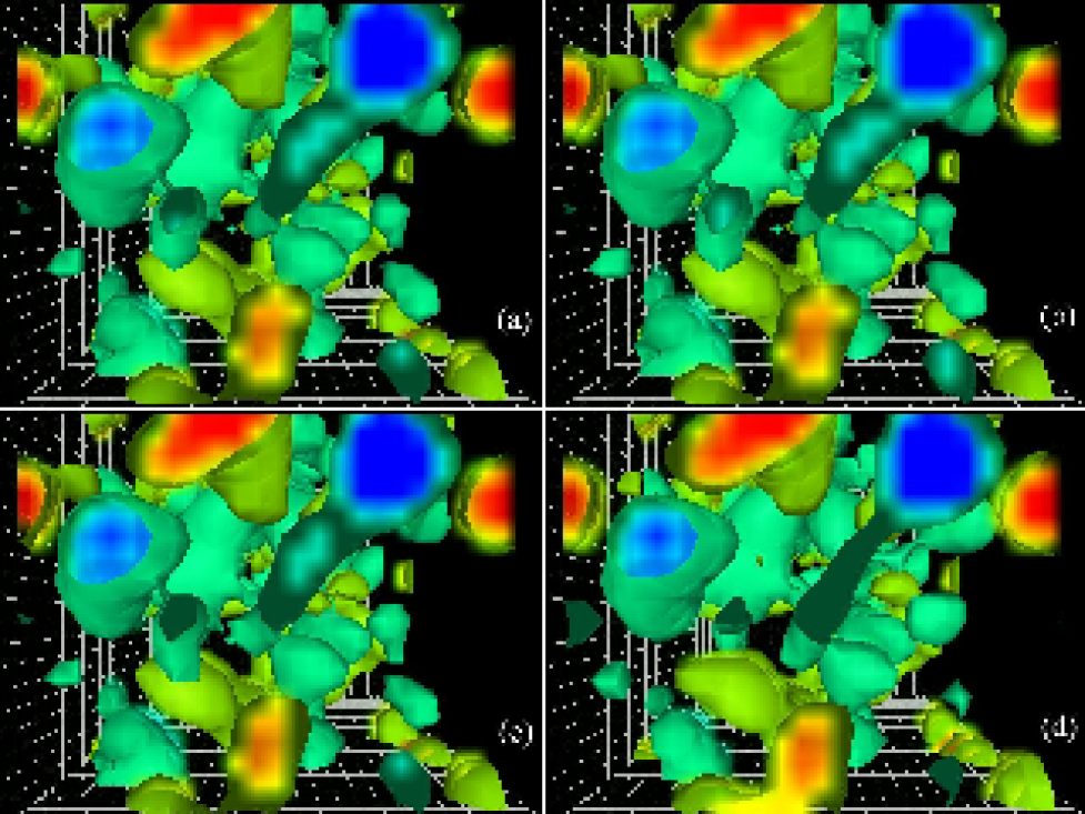
FIG. 22.: Topological charge density of a $24^{3}\times{36}$ lattice for fixed $x$ coordinate. Positive (negative) windings are colored red to yellow (blue to green). Fig. (a) illustrates the topological charge density after 21 APE smearing steps at $\alpha=0.7$. Fig. (b) illustrates the topological charge density after 49 APE smearing steps at $\alpha=0.3$. Relation (20) suggests these configurations should be similar and we see they are to a remarkable level of detail. Fig. (c) illustrates the topological charge density after 20 AUS smearing steps at $\alpha=0.7$. Relation (24) suggests these configurations should be similar and again the detail of the agreement is excellent. Finally (d) illustrates the topological charge density after 9 cooling sweeps, motivated by relation (23). While the level of agreement is not as precise, the qualitative features of the smoothed configurations are compatible.

V Conclusion

The APE smearing algorithm is now widely used in a variety of ways in lattice simulations. It is used to smear the spatial gauge-field links in studies of glueballs, hybrid mesons, the static quark potential, etc. It is used in constructing fat-link actions and in constructing improved operators with smooth transitions to the continuum limit. We have shown that to a good approximation the two-dimensionful parameter space of the number of smearing sweeps $n_{\rm{ape}}(\alpha)$ and the smearing fraction $\alpha$ may be reduced to a single dimension via the constraint

$$\frac{n_{\rm{ape}}(\alpha^{\prime})}{n_{\rm{ape}}(\alpha)}=\frac{\alpha}{\alpha^{\prime}}\,.$$ (28)

satisfied for $\alpha$ and $\alpha^{\prime}$ in the range 0.3 to 0.7. This result is in agreement with fat-link perturbation theory expectations, and survives for up to 200 sweeps over the lattice. We expect this relation to hold over the entire APE smearing range $0<\alpha<3/4$. We find the same relation for AUS smearing provided $\alpha\leq 0.85$. For AUS smearing, annealing of the links is included as one cycles through the Lorentz directions of the link variables in the smearing process.

The smoothing of gauge field configurations is often a necessary step in extracting observables in which the renormalization constants differ significantly from one, as is the case for the topological charge operator. It is also often used to gain insights into the nonperturbative features of the field theory which give rise to the observed phenomena. We have determined that cooling, APE smearing and AUS smearing produce qualitatively similar smoothed gauge field configurations at $\beta=6.0$ provided one calibrates the algorithms as follows:

$$n_{c}\simeq 0.600\,\alpha\,{n_{\rm{ape}}(\alpha)}\,,\hskip 15.6491ptn_{c}\simeq 0.618\,\alpha\,{n_{\rm{aus}}(\alpha)}\,\hskip 15.6491pt{\rm and}\hskip 15.6491pt\alpha\,{n_{\rm{ape}}(\alpha)}\simeq 1.03\,\alpha^{\prime}\,{n_{\rm{aus}}(\alpha^{\prime})}\,.$$ (29)

The topological charge analysis serves to confirm the action analysis results at $\beta=6.0$ and further support these relations. However, it also reveals that at $\beta=5.7$ different trajectories are taken. At $\beta=5.7$ different algorithms produce smoothed gauge field configurations with similar action, but different topological properties.

As most modern simulations are performed at $\beta\geq 6.0$, the relations of Eqs. (28) and (29) will be most effective in reducing the exploration of the parameter space. It is now possible to arrive at optimal smearing by fixing the number of smearing sweeps and varying the smearing fraction, or vice versa. Finally, it is now possible to directly compare the physics of smeared and cooled gauge field configurations in a quantitative sense.

We have used the action and topological charge trajectories to calibrate the various smoothing algorithms. While the topological charge may be related to the topological susceptibility, it may be of future interest to introduce other physical quantities such as the string tension as a measure of smoothing [8].

It is well known that interpreting the physics of cooled configurations based on the standard Wilson action is somewhat of an art. The difficulty is that the ${\cal O}(a^{2})$ errors in the action spoil an instanton under cooling by reducing the action below the one-instanton bound. A consequence of this is a lack of universality. For example, the action varies smoothly to zero while the topological sector jumps as (anti)instantons are destroyed. One may then attempt to define the concept of an optimal amount of smoothing, and perhaps also extrapolate back to zero smoothing steps. Unfortunately, all of these difficulties are apparent in the APE smearing analysis results as well.

Because of the intimate connection between smearing and cooling, as emphasized in the discussion of Section III B 2, it is natural to consider improved smearing, where the Hermitian conjugate of the improved staple is used in the smearing process. It will be interesting to see if the benefits of improved cooling carry over into improved smearing and this work is currently in progress.

REFERENCES

- [1] B. Berg, Phys. Lett. B104, 475 (1981). M. Teper, Phys. Lett. B162, 357 (1985); B171 81, 86 (1986). E. M. Ilgenfritz et al, Nucl. Phys. B268 693 (1986).
- [2] Campostrini M. et al, Phys. Lett. B212, 206 (1988); B. Alles, M. D’Elia and A. Di Giacomo, Nucl. Phys. B494, 281 (1997).
- [3] M. Falcioni, M. Paciello, G. Parisi, B. Taglienti, Nucl. Phys. B251, 624 (1985); M. Albanese et al, Phys. Lett. B192, 163 (1987).
- [4] C. Bernard and T. DeGrand, “Perturbation theory for fat-link fermion actions,” hep-lat/9909083.
- [5] A. di Giacomo et al., Nucl. Phys. (Proc. Suppl.) 54A, 343 (1997), hep-lat/9608014.
- [6] A. Ringwald and F. Schrempp, Phys. Lett. B459, 249 (1999), hep-lat/9903039.
- [7] Philippe de Forcrand, Margarita G. Perez and Ion-Olimpiu Stamatescu, Nucl. Phys. B499 409 (1997) hep-lat/9701012; P. de Forcrand, M. Garcia Perez, J. E. Hetrick and I. Stamatescu, “Topological properties of the QCD vacuum at T = O and T approx. T(c),” hep-lat/9802017.
- [8] M. Garcia Perez et al., Nucl. Phys. B551, 293 (1999), hep-lat/9812006.
- [9] D.A. Smith and M. Teper, Phys. Rev. D58, 014505 (1998), hep-lat/9801008.
- [10] N. Cabibbo and E. Marinari, Phys. Lett. B 119, 387 (1982).
- [11] Lattice 98, Nucl. Phys. B (Proc. Suppl.) 73 (1999).
- [12] J. E. Hetrick and P. de Forcrand, Nucl. Phys. Proc. Suppl. 63, 838 (1998) hep-lat/9710003.
- [13] T. DeGrand [MILC collaboration], Phys. Rev. D60, 094501 (1999) hep-lat/9903006.
- [14] D. B. Leinweber, J. I. Skullerud, A. G. Williams and C. Parrinello [UKQCD Collaboration], Phys. Rev. D60, 094507 (1999) hep-lat/9811027; D. B. Leinweber, J. I. Skullerud, A. G. Williams and C. Parrinello [UKQCD collaboration], Phys. Rev. D58, 031501 (1998) hep-lat/9803015; See also J.E. Mandula, Phys. Rept. 315 273, (1999) and references therein.