Fast methods for computing the Neuberger Operator

Abstract

I describe a Lanczos method to compute the Neuberger Operator and a multigrid algorithm for its inversion.

1 Introduction

Quantum Chromodynamics (QCD) is a theory of strong interactions, where the chiral symmetry plays a mayor role. There are different starting points to formulate a lattice theory with exact chiral symmetry, but all of them must obey the Ginsparg-Wilson condition [1]:

$$\gamma_{5}D^{-1}+D^{-1}\gamma_{5}=a\gamma_{5}{\alpha}^{-1},$$ (1)

where $a$ is the lattice spacing, $D$ is the lattice Dirac operator and ${\alpha}^{-1}$ is a local operator and trivial in the Dirac space.

A candidate is the overlap operator of Neuberger [2]:

$$D=1-A(A^{{\dagger}}A)^{-1/2},~{}~{}~{}~{}A=M-aD_{W}$$ (2)

where $M$ is a shift parameter in the range $(0,2)$, which I have fixed at one and $D_{W}$ is the Wilson-Dirac operator,

$$D_{W}=\frac{1}{2}\sum_{\mu}[\gamma_{\mu}(\partial_{\mu}^{*}+\partial_{\mu})-a\partial_{\mu}^{*}\partial_{\mu}]$$ (3)

and $\partial_{\mu}$ and $\partial_{\mu}^{*}$ are the nearest-neighbor forward and backward difference operators, which are covariant, i.e. the shift operators pick up a unitary 3 by 3 matrix with determinant one. These small matrices are associated with the links of the lattice and are oriented positively. A set of such matrices forms a ”configuration”. $\gamma_{\mu},\mu=1,\ldots,5$ are 4 by 4 matrices related to the spin of the particle. Therefore, if there are $N$ lattice points, the matrix is of order $12N$. A restive symmetry of the matrix $A$ that comes from the continuum is the so called $\gamma_{5}-symmetry$ which is the Hermiticity of the $\gamma_{5}A$ operator.

The computation of the inverse square root of a matrix is reviewed in [3]. In the context of lattice QCD there are several sparse matrix methods, which are developed recently [4, 5, 6, 7, 8]. I will focus here on a Lanczos method similar to [4]. For a more general case of functions of matrices I refer to the talk of H. van der Vorst, and for a Chebyshev method I refer to the talk of K. Jansen, both included in these proceedings.

2 The Lanczos Algorithm

The Lanczos iteration is known to approximate the spectrum of the underlying matrix in an optimal way and, in particular, it can be used to solve linear systems [9].

Let $Q_{n}=[q_{1},\ldots,q_{n}]$ be the set of orthonormal vectors, such that

$$A^{{\dagger}}AQ_{n}=Q_{n}T_{n}+\beta_{n}q_{n+1}(e_{n}^{(n)})^{T},~{}~{}~{}~{}q_{1}=\rho_{1}b,~{}~{}~{}~{}\rho_{1}=1/||b||_{2}$$ (4)

where $T_{n}$ is a tridiagonal and symmetric matrix, $b$ is an arbitrary vector, and $\beta_{n}$ a real and positive constant. $e_{m}^{(n)}$ denotes the unit vector with $n$ elements in the direction $m$.

By writing down the above decomposition in terms of the vectors $q_{i},i=1,\ldots,n$ and the matrix elements of $T_{n}$, I arrive at a three term recurrence that allows to compute these vectors in increasing order, starting from the vector $q_{1}$. This is the $LanczosAlgorithm$:

$$\begin{array}[]{l}\beta_{0}=0,~{}\rho_{1}=1/||b||_{2},~{}q_{0}=o,~{}q_{1}=\rho_{1}b\\ for~{}i=1,\ldots\\ ~{}~{}~{}~{}v=A^{{\dagger}}Aq_{i}\\ ~{}~{}~{}~{}\alpha_{i}=q_{i}^{{\dagger}}v\\ ~{}~{}~{}~{}v:=v-q_{i}\alpha_{i}-q_{i-1}\beta_{i-1}\\ ~{}~{}~{}~{}\beta_{i}=||v||_{2}\\ ~{}~{}~{}~{}if\beta_{i}<tol,~{}n=i,~{}end~{}for\\ ~{}~{}~{}~{}q_{i+1}=v/\beta_{i}\\ \end{array}$$ (5)

where $tol$ is a tolerance which serves as a stopping condition.

The Lanczos Algorithm constructs a basis for the Krylov subspace [9]:

$$\mbox{span}\{b,A^{{\dagger}}Ab,\ldots,(A^{{\dagger}}A)^{n-1}b\}$$ (6)

If the Algorithm stops after $n$ steps, one says that the associated Krylov subspace is invariant.

In the floating point arithmetic, there is a danger that once the Lanczos Algorithm (polynomial) has approximated well some part of the spectrum, the iteration reproduces vectors which are rich in that direction [9]. As a consequence, the orthogonality of the Lanczos vectors is spoiled with an immediate impact on the history of the iteration: if the algorithm would stop after $n$ steps in exact arithmetic, in the presence of round off errors the loss of orthogonality would keep the algorithm going on.

3 The Lanczos Algorithm for solving $A^{{\dagger}}Ax=b$

Here I will use this algorithm to solve linear systems, where the loss of orthogonality will not play a role in the sense that I will use a different stopping condition.

I ask the solution in the form

$$x=Q_{n}y_{n}$$ (7)

By projecting the original system on to the Krylov subspace I get:

$$Q_{n}^{{\dagger}}A^{{\dagger}}Ax=Q_{n}^{{\dagger}}b$$ (8)

By construction, I have

$$b=Q_{n}e_{1}^{(n)}/\rho_{1},$$ (9)

Substituting $x=Q_{n}y_{n}$ and using (4), my task is now to solve the system

$$T_{n}y_{n}=e_{1}^{(n)}/\rho_{1}$$ (10)

Therefore the solution is given by

$$x=Q_{n}T_{n}^{-1}e_{1}^{(n)}/\rho_{1}$$ (11)

This way using the Lanczos iteration one reduces the size of the matrix to be inverted. Moreover, since $T_{n}$ is tridiagonal, one can compute $y_{n}$ by short recurences.

If I define:

$$r_{i}=b-A^{{\dagger}}Ax_{i},~{}~{}q_{i}=\rho_{i}r_{i},~{}~{}y_{i}=\rho_{i}x_{i}$$ (12)

where $i=1,\ldots$, it is easy to show that

$$\begin{array}[]{l}\rho_{i+1}\beta_{i}+\rho_{i}\alpha_{i}+\rho_{i-1}\beta_{i-1}=0\\ q_{i}+y_{i+1}\beta_{i}+y_{i}\alpha_{i}+y_{i-1}\beta_{i-1}=0\end{array}$$ (13)

Therefore the solution can be updated recursively and I have the following Algorithm1 for solving the system $A^{{\dagger}}Ax=b$:

$$\begin{array}[]{l}\beta_{0}=0,~{}\rho_{1}=1/||b||_{2},~{}q_{0}=o,~{}q_{1}=\rho_{1}b\\ for~{}i=1,\ldots\\ ~{}~{}~{}~{}v=A^{{\dagger}}Aq_{i}\\ ~{}~{}~{}~{}\alpha_{i}=q_{i}^{{\dagger}}v\\ ~{}~{}~{}~{}v:=v-q_{i}\alpha_{i}-q_{i-1}\beta_{i-1}\\ ~{}~{}~{}~{}\beta_{i}=||v||_{2}\\ ~{}~{}~{}~{}q_{i+1}=v/\beta_{i}\\ ~{}~{}~{}~{}y_{i+1}=-\frac{q_{i}+y_{i}\alpha_{i}+y_{i-1}\beta_{i-1}}{\beta_{i}}\\ ~{}~{}~{}~{}\rho_{i+1}=-\frac{\rho_{i}\alpha_{i}+\rho_{i-1}\beta_{i-1}}{\beta_{i}}\\ ~{}~{}~{}~{}r_{i+1}:=q_{i+1}/\rho_{i+1}\\ ~{}~{}~{}~{}x_{i+1}:=y_{i+1}/\rho_{i+1}\\ ~{}~{}~{}~{}if\frac{1}{|\rho_{i+1}|}<tol,~{}n=i,~{}end~{}for\\ \end{array}$$ (14)

4 The Lanczos Algorithm for solving $(A^{{\dagger}}A)^{1/2}x=b$

Now I would like to compute $x=(A^{{\dagger}}A)^{-1/2}b$ and still use the Lanczos Algorithm. In order to do so I make the following observations:

Let $(A^{{\dagger}}A)^{-1/2}$ be expressed by a matrix-valued function, for example the integral formula [3]:

$$(A^{{\dagger}}A)^{-1/2}=\frac{2}{\pi}\int_{0}^{\infty}dt(t^{2}+A^{{\dagger}}A)^{-1}$$ (15)

From the previous section, I use the Lanczos Algorithm to compute

$$(A^{{\dagger}}A)^{-1}b=Q_{n}T_{n}^{-1}e_{1}^{(n)}/\rho_{1}$$ (16)

It is easy to show that the Lanczos Algorithm is shift-invariant. i.e. if the matrix $A^{{\dagger}}A$ is shifted by a constant say, $t^{2}$, the Lanczos vectors remain invariant. Moreover, the corresponding Lanczos matrix is shifted by the same amount.

This property allows one to solve the system $(t^{2}+A^{{\dagger}}A)x=b$ by using the same Lanczos iteration as before. Since the matrix $(t^{2}+A^{{\dagger}}A)$ is better conditioned than $A^{{\dagger}}A$, it can be concluded that once the original system is solved, the shifted one is solved too. Therefore I have:

$$(t^{2}+A^{{\dagger}}A)^{-1}b=Q_{n}(t^{2}+T_{n})^{-1}e_{1}^{(n)}/\rho_{1}$$ (17)

Using the above integral formula and puting everything together, I get:

$$x=(A^{{\dagger}}A)^{-1/2}b=Q_{n}T_{n}^{-1/2}e_{1}^{(n)}/\rho_{1}$$ (18)

There are some remarks to be made here:

a) As before, by applying the Lanczos iteration on $A^{{\dagger}}A$, the problem of computing $(A^{{\dagger}}A)^{-1/2}b$ reduces to the problem of computing $y_{n}=T_{n}^{-1/2}e_{1}^{(n)}/\rho_{1}$ which is typically a much smaller problem than the original one. But since $T_{n}^{1/2}$ is full, $y_{n}$ cannot be computed by short recurences. It can be computed for example by using the full decomposition of $T_{n}$ in its eigenvalues and eigenvectors; in fact this is the method I have employed too, for its compactness and the small overhead for moderate $n$.

b) The method is not optimal, as it would have been, if one would have applied it directly for the matrix $(A^{{\dagger}}A)^{1/2}$. By using $A^{{\dagger}}A$ the condition is squared, and one looses a factor of two compared to the theoretical case!

c) From the derivation above, it can be concluded that the system $(A^{{\dagger}}A)^{1/2}x=b$ is solved at the same time as the system $A^{{\dagger}}Ax=b$.

d) To implement the result (18), I first construct the Lanczos matrix and then compute

$$y_{n}=T_{n}^{-1/2}e_{1}^{(n)}/\rho_{1}$$ (19)

To compute $x=Q_{n}y_{n}$, I repeat the Lanczos iteration. I save the scalar products, though it is not necessary.

Therefore I have the following Algorithm2 for solving the system $(A^{{\dagger}}A)^{1/2}x=b$:

$$\begin{array}[]{l}\beta_{0}=0,~{}\rho_{1}=1/||b||_{2},~{}q_{0}=o,~{}q_{1}=\rho_{1}b\\ for~{}i=1,\ldots\\ ~{}~{}~{}~{}v=A^{{\dagger}}Aq_{i}\\ ~{}~{}~{}~{}\alpha_{i}=q_{i}^{{\dagger}}v\\ ~{}~{}~{}~{}v:=v-q_{i}\alpha_{i}-q_{i-1}\beta_{i-1}\\ ~{}~{}~{}~{}\beta_{i}=||v||_{2}\\ ~{}~{}~{}~{}q_{i+1}=v/\beta_{i}\\ ~{}~{}~{}~{}\rho_{i+1}=-\frac{\rho_{i}\alpha_{i}+\rho_{i-1}\beta_{i-1}}{\beta_{i}}\\ ~{}~{}~{}~{}if\frac{1}{|\rho_{i+1}|}<tol,~{}n=i,~{}end~{}for\\ \\ Set~{}(T_{n})_{i,i}=\alpha_{i},~{}(T_{n})_{i+1,i}=(T_{n})_{i,i+1}=\beta_{i},otherwise~{}(T_{n})_{i,j}=0\\ y_{n}=T_{n}^{-1/2}e_{1}^{(n)}/\rho_{1}=U_{n}\Lambda_{n}^{-1/2}U_{n}^{T}e_{1}^{(n)}/\rho_{1}\\ \\ q_{0}=o,~{}q_{1}=\rho_{1}b,~{}x_{0}=o\\ for~{}i=1,\ldots,n\\ ~{}~{}~{}~{}x_{i}=x_{i-1}+q_{i}y_{n}^{(i)}\\ ~{}~{}~{}~{}v=A^{{\dagger}}Aq_{i}\\ ~{}~{}~{}~{}v:=v-q_{i}\alpha_{i}-q_{i-1}\beta_{i-1}\\ ~{}~{}~{}~{}q_{i+1}=v/\beta_{i}\\ \end{array}$$ (20)

where by $o$ I denote a vector with zero entries and $U_{n},\Lambda_{n}$ the matrices of the egienvectors and eigenvalues of $T_{n}$. Note that there are only four large vectors necessary to store: $q_{i-1},q_{i},v,x_{i}$.

5 Testing the method

I propose a simple test: I solve the system $A^{{\dagger}}Ax=b$ by applying twice the $Algorithm2$, i.e. I solve the linear systems

$$(A^{{\dagger}}A)^{1/2}z=b,~{}~{}(A^{{\dagger}}A)^{1/2}x=z$$ (21)

in the above order. For each approximation $x_{i}$, I compute the residual vector

$$r_{i}=b-A^{{\dagger}}Ax_{i}$$ (22)

The method is tested for a SU(3) configuration at $\beta=6.0$ on a $8^{3}16$ lattice, corresponding to an order $98304$ complex matrix $A$.

In Fig.1 I show the norm of the residual vector decreasing monotonically. The stagnation of $||r_{i}||_{2}$ for small values of $tol$ may come from the accumulation of round off error in the $64$-bit precision arithmetic used here.

This example shows that the tolerance line is above the residual norm line, which confirms the expectation that $tol$ is a good stopping condition of the $Algorithm2$.

6 Inversion

Having computed the operator, one can invert it by applying iterative methods based on the the Lanczos algorithm. Since the operator $D$ is normal, it turns out that the Conjugate Residual (CR) algorithm is the optimal one [10].

In Fig. 2 I show the converegence history of CR on $30$ small $4^{4}$ lattices at $\beta=6$. The large number of multiplications with $D_{W}$ suggests that the inversion of the Neuberger operator is a difficult task and may bring the complexity of quenched simulations in lattice QCD to the same order of magnitude to dynamical simulations with Wilson fermions.

Therefore, other ideas are needed.

The essential point is the large number of small eigenvalues of $A$ that make the computation of $D$ time consuming. Therefore, one may try to project out these modes and invert them directly [11].

Also, one may try $5-$dimensional implementations of the Neuberger operator, such that its condition improves [12].

I have tried also to reformulate the theory in 5 dimensions by using the corresponding approximate inversion as a coarse grid solution in a multigrid scheme [13].

The scheme is tested and the results are shown in Fig. 2, where the multigrid pattern of the residual norm is clear. The gain with respect to CR is about a factor $10$.

Note that to invert the “big” matrix I have used the BiCGstab2 algorithm [14] which is almost optimal in most of the cases for the non-normal matrices as its is the matrix $\cal M$ [10].

7 Acknowledgement

The author would like to thank the organizers of this Workshop for the kind hospitality at Wuppertal.

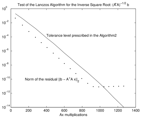
Figure 1: The dots show the norm of the residual vector, whereas the line shows the tolerance level set by $tol$ in the $Algorithm2$.

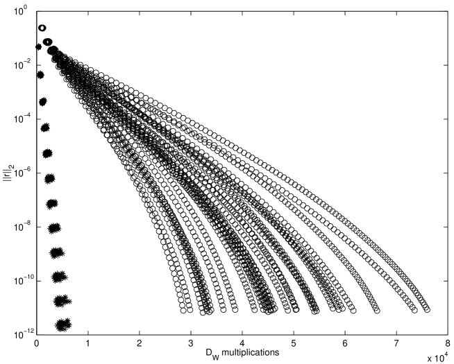
Figure 2: Norm of the residual error vs. the number of $D_{W}$ multiplications on 30 configurations. Circles stand for the straightforward inversion with CR and stars for the multigrid algorithm.

References

- [1] P. H. Ginsparg and K. G. Wilson, Phys. Rev. D 25 (1982) 2649.
- [2] H. Neuberger, Phys. Lett. B 417 (1998) 141, Phys. Rev. D 57 (1998) 5417.
- [3] N. J. Higham, Proceedings of ”Pure and Applied Linear Algebra: The New Generation”, Pensacola, March 1993.
- [4] A. Boriçi, Phys.Lett. B453 (1999) 46-53, hep-lat/9910045
- [5] H. Neuberger, Phys. Rev. Lett. 81 (1998) 4060.
- [6] R. G. Edwards, U. M. Heller and R. Narayanan, Nucl.Phys. B540 (1999) 457-471.
- [7] B. Bunk, Nucl.Phys.Proc.Suppl. B63 (1998) 952.
- [8] P. Hernandes, K. Jansen, L. Lellouch, these proceedings and hep-lat/0001008.
- [9] G. H. Golub and C. F. Van Loan, Matrix Computations, The Johns Hopkins University Press, Baltimore, 1989. This is meant as a general reference with original references included therein.
- [10] A. Boriçi, Krylov Subspace Methods in Lattice QCD, PhD Thesis, CSCS TR-96-27, ETH Zürich 1996.
- [11] R. G. Edwards, U. M. Heller, J. Kiskis, R. Narayanan, hep-lat/9912042.
- [12] H. Neuberger, hep-lat/9909042
- [13] A. Boriçi, hep-lat/9907003, hep-lat/9909057
- [14] M. H. Gutknecht, SIAM J. Sci. Comput., 14 (1993) 1020.