General Algorithm For Improved Lattice Actions on Parallel Computing Architectures

Abstract

Quantum field theories underlie all of our understanding of the fundamental forces of nature. The are relatively few first principles approaches to the study of quantum field theories [such as quantum chromodynamics (QCD) relevant to the strong interaction] away from the perturbative (i.e., weak-coupling) regime. Currently the most common method is the use of Monte Carlo methods on a hypercubic space-time lattice. These methods consume enormous computing power for large lattices and it is essential that increasingly efficient algorithms be developed to perform standard tasks in these lattice calculations. Here we present a general algorithm for QCD that allows one to put any planar improved gluonic lattice action onto a parallel computing architecture. High performance masks for specific actions (including non-planar actions) are also presented. These algorithms have been successfully employed by us in a variety of lattice QCD calculations using improved lattice actions on a 128 node Thinking Machines CM-5.

Keywords: quantum field theory; quantum chromodynamics; improved actions; parallel computing algorithms.

I Introduction

It is almost universally accepted that Quantum Chromodynamics (QCD) is the underlying quantum field theory of the strong interaction [1, 2], which binds atomic nuclei and fuels the sun and the stars. Strongly interacting particles are referred to as hadrons, which include for example protons and neutrons that make up atomic nuclei as well as a wide variety of particles that are produced in particle accelerators and from astrophysical sources. These hadrons are made up of quarks and gluons, which are the underlying constituents in QCD. The quarks are spin-1/2 particles (i.e., fermions) and the gluons are massless spin-1 particles (i.e., gauge bosons). The quarks interact strongly through their “colour” charge through the exchange of gluons. The 8 gluons of SU(3) (i.e., one for each generator of SU(3)) themselves carry colour and hence interact with themselves as well as with the quarks. This is the essential difference between QCD and the corresponding theory of photons and electrons referred to as quantum electrodynamics (QED) and has far reaching consequences since the theories have entirely different behavior.

The are very few first-principles methods for studying QCD in the nonperturbative low-energy regime. The most widely used of these is the so-called Lagrangian-based lattice field theory, which formulates the field theory on a space-time lattice [3, 4]. An alternative lattice approach is based on the Hamiltonian formulation of quantum field theory and makes use of cluster decompositions and again Monte Carlo methods to carry out the simulations[5]. In addition, there are numerous studies based on a light-front formulation of QCD [6] and much use has been made of Schwinger-Dyson equations[7] to assist with the construction of QCD-based quark models.

The Lagrangian-based lattice technique simulates the functional integral using a four-dimensional hypercubic Euclidean spacetime lattice together with Monte Carlo methods for generating an ensemble of gluon field configurations with the appropriate Boltzmann distribution $\exp(-S_{G})$, where $S_{G}$ is a discretized form of the QCD gluon action on the hypercubic lattice. The simplest discretizations of the QCD action involve only nearest neighbours on the lattice and have ${\cal O}(a^{2})$ errors, where $a$ is the lattice spacing. Improved actions represent a major advance for the field of lattice gauge theory, where by using increasingly non-local discretizations of the QCD action we can obtain the same accuracy with far fewer lattice points and hence far less computational time and effort. The purpose of the present work is to describe an algorithm which allows us to implement an arbitrarily improved (i.e., arbitrarily non-local) action in an efficient way. For further details on the state of the art lattice QCD techniques see for example Ref. [8]. Another related and equally important advance is the technique of nonperturbative improvement (e.g., mean-field improvement) which corrects for some of the major nonperturbative effects (the so-called tadpole contributions) and hence more quickly brings the lattice results to their continuum form by improving the matching with perturbation theory at a given lattice spacing $a$ [9]. It is the combination of improved actions and nonperturbative improvement that together have come to represent a significant advance for the field [8, 10].

Lattice QCD is based on a Monte Carlo treatment of the path integral formulation, which makes it a computationally demanding method for calculating physical observables. The gluon field is represented by $3\times 3$ complex $SU(3)$ matrices, where there is one such $SU(3)$ matrix associated with every link on the lattice. The links lie only along one of the four Cartesian directions and join neighbouring lattice sites. Since all lattice links require identical numerical calculations, lattice gauge theory is ideally suited for parallel computers.

There are various types of improved actions and, as explained above, these are all based on the idea of eliminating the discretization errors that occur when passing from continuum physics to the discretized lattice version. The simplest (i.e., non-improved) gluon action is the so called standard Wilson action and consists of $1\times{1}$ Wilson loops or as they are frequently called plaquettes. We shall often refer to the Wilson loops used to build up lattice actions as plaquettes. The need to build the gluon action out of closed loops arises from the need to maintain exact $SU(3)$ gauge invariance in the discrete lattice action. This $1\times{1}$ loop action was first proposed by Wilson [11] in the early 70’s and has been used extensively over the years. It consists of taking an arbitrary starting site, say $x$, on the lattice and stepping around a $1\times{1}$ loop until returning to the starting point $x$. The $1\times{1}$ Wilson loop is illustrated in Fig. 1.

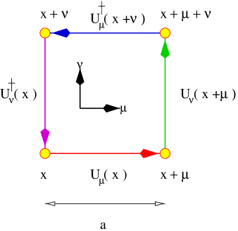
FIG. 1.: The $1\times 1$ plaquette $U_{\rm{sq}}(x)$ with base at $x$ lying in the $\mu\nu$-plane. The lattice spacing is denoted by $a$.

Improving the standard Wilson action is achieved by making use of larger loops (e.g., $1\times 2$, $2\times 2$, etc.) in the lattice gluon action[12] to eliminate finite lattice spacing artifacts to a given order in $a^{2}$ . For an elegant and detailed discussion of these topics see Ref. [10].

In this article we present an efficient and completely general algorithm that permits one to calculate any improved planar lattice action at any desired level of improvement. By “planar” here we mean that we will consider actions containing two-dimensional loops of arbitrary size which lie in any of the Cartesian planes, (i.e., the $x-y$, $x-z$, $x-t$, $y-z$, $y-t$, or $z-t$ plane). This algorithm has been used in a wide variety of improved action lattice simulations to date [8]. For example, it has been used in studies of the topological structure of the QCD vacuum and the calibration of the various cooling and smearing techniques [13], the study of discretization errors in the Landau gauge on the lattice [14], and studies of the static quark potential [15]. It is currently being used in studies of the gluon propagator [16] and highly improved actions [17].

In Sec. II, we briefly describe the tree–level improved action that we have been using in our calculations [13, 14, 15, 16, 17] with our algorithm on a Thinking Machines CM-5. Sec. III gives two possible ways of using the technique for the standard Wilson action. The form of the algorithm appropriate for the first level of improvement (i.e., involving a combination of the elementary square $1\times 1$ plaquette and the rectangular $1\times 2$ plaquette) is given in Sec. IV. Then in Sec. V we present the general algorithm suitable for an arbitrarily non-local action, (i.e., for an $n\times m$ Wilson loop with $n$ and $m$ being arbitrary positive integers). Sec. VI addresses non-planar issues encountered in nesting specific planar actions. Actions involving non-planar loops are also addressed. Finally, in Sec. VII we present our summary and conclusions.

II Gauge Action, Masking, and Parallel Computing

A Lattice Gauge Action for Colour $SU(3)$

The standard Wilson action for the gluons is given by

$$S^{\rm W}_{G}=\beta\sum_{\rm{sq}}\left[1-\frac{1}{3}{\cal R}e{\rm Tr}U_{\rm{sq}}(x)\right]$$ (1)

and a simple tree–level ${\cal O}(a^{2})$–improved action (i.e., the action with the first level of improvement) is defined as

$$S_{G}=\frac{5\beta}{3}\sum_{\rm{sq}}{\cal R}e{\rm Tr}(1-U_{\rm{sq}}(x))-\frac{\beta}{12u_{0}^{2}}\sum_{\rm{rect}}{\cal R}e{\rm Tr}(1-U_{\rm{rect}}(x))\,.$$ (2)

The $1\times{1}$ square (or plaquette) $U_{\rm{sq}}(x)$ and the $1\times 2$ rectangle $U_{\rm{rect}}(x)$ are defined by

$$U_{\rm{sq}}(x) = U_{\mu}(x)U_{\nu}(x+\hat{\mu})U^{\dagger}_{\mu}(x+\hat{\nu})U^{\dagger}_{\nu}(x)$$ (3)

$$U_{\rm{rect}}(x) = U_{\mu}(x)U_{\nu}(x+\hat{\mu})U_{\nu}(x+\hat{\nu}+\hat{\mu})U^{\dagger}_{\mu}(x+2\hat{\nu})U^{\dagger}_{\nu}(x+\hat{\nu})U^{\dagger}_{\nu}(x)$$ (4)

$$+ U_{\mu}(x)U_{\mu}(x+\hat{\mu})U_{\nu}(x+2\hat{\mu})U^{\dagger}_{\mu}(x+\hat{\mu}+\hat{\nu})U^{\dagger}_{\mu}(x+\hat{\nu})U^{\dagger}_{\nu}(x).$$ (5)

Here the variables $\mu$ and $\nu$ are the direction in which the links are pointing inside the lattice space. There are four directions for a four-dimensional hypercubic lattice. The link product $U_{\rm{rect}}(x)$ denotes the rectangular $1\times 2$ plaquettes and $u_{0}$ is the tadpole improvement factor, commonly known as the mean–field improvement factor which largely corrects for quantum renormalization of the links. In our numerical studies we have typically employed the plaquette definition of the mean–field improvement factor

$$u_{0}=\left(\frac{1}{3}{\cal R}e{\rm Tr}\langle U_{\rm{sq}}\rangle\right)^{\frac{1}{4}}.$$ (6)

For the improved action in Eq. (2) the residual perturbative corrections after mean–field improvement are estimated to be of the order of two to three percent [18]. Of course, both Eqs. (1) and (2) reproduce the continuum gluon action as $a\rightarrow{0}$, where $\beta\equiv 6/g^{2}$ and $g$ is the QCD coupling constant at the scale $a$. It is useful to note that our $\beta=6/g^{2}$ differs from the convention of Refs. [18, 19, 20]. A multiplication of our $\beta$ in Eq. (2) by a factor of $5/3$ reproduces their definition.

Let us comment on the lattice configurations that we have generated with the general algorithm described here and which we have used extensively in Refs. [13, 14, 15, 16, 17]. The gauge configurations are generated using the Cabbibo-Marinari [21] pseudo–heat–bath algorithm with three diagonal $SU_{c}(2)$ subgroups. All calculations are performed using a highly parallel code written in CM-Fortran and run on a Thinking Machines Corporations (TMC) CM-5 with appropriate link partitioning. For the standard Wilson action we partition the link variable in a checkerboard fashion. While all calculations to date have been for $SU(3)$, there is no restriction in the algorithm on the number of colours for the gauge group [21] and we could just has easily have treated the case of $SU(N)$.

The mean–field improvement factor was updated on a regular basis during the simulation. Once the lattice is thermalized from a cold start, (after at least five thousand sweeps), the $u_{0}$ factor is held fixed during the generation of the ensemble of gauge field configurations. The ensemble is built up by sampling the fields with a separation of at least 500 Monte Carlo sweeps over the entire lattice to ensure that they are sufficiently decorrelated. For the case of the standard Wilson action, configurations have been generated on a $16^{3}\times 32$ lattice at $\beta=5.70$ and a $24^{3}\times 36$ lattice at $\beta=6.00$. For the improved action of Eq. (2) we have generated $8^{3}\times 16$, $12^{3}\times 24$, $16^{3}\times 32$, and $24^{3}\times 36$ lattices with $\beta$ values of 3.57, 4.10, 4.38, and 5.00 respectively.

B Masking and Parallel Computing

When performing a Monte Carlo sweep of the entire lattice each lattice link must be updated individually using the particular gluon action of interest (e.g., $S_{G}$). The action is used in the Monte Carlo accept/reject step for that link in order that detailed balance is ensured at each link update and hence that it is ensured throughout the entire lattice sweep. It is the combination of randomness in the link updates, the maintenance of detailed balance, and decorrelation (ensured by large sweep numbers between the taking of samples) that ensures the desired ensemble of gauge field configurations are produced with the Boltzmann distribution $\exp(-S_{G})$.

In the most naive procedure we move through each link on the lattice consecutively updating them one at a time until we have completed a “sweep” through the entire lattice. We then repeat these lattice sweeps as often as required. This simple procedure is highly inefficient on a parallel computing architecture, where we can be updating many links at the same time. However, there is a fundamental limitation to this parallelism, i.e., we will violate detailed balance and corrupt our data if we try to simultaneously update a link while information about that link is being used in the update of another link. It is crucial that we identify which links can be updated simultaneously and this is determined by the degree of non locality in the action. For example, for an action which contains only nearest neighbor interactions of the links, such as the Wilson action, we can use an efficient “checkerboard” algorithm, which will be described below. In general, the more non local is the lattice gluon action the fewer are the links that can be simultaneously updated. We see that the improvement program is therefore more expensive to implement, but the benefit of improved actions far outweighs this drawback.

In order to facilitate our discussions we will refer to the concept of “masking”, where the lattice links not eliminated by the mask are the ones that can be simultaneously updated in a parallel computing environment. The number of independent masks needed for a particular action determines an upper limit to the parallelism that can be used in a single lattice sweep. As we will see, the best that can be done is to have two masks per link direction and this is for the case of nearest neighbor interactions only.

We will simplify the presentation in the usual way by rescaling all dimensionful quantities by the lattice spacing $a$. This is equivalent to setting $a=1$.

III Masking for the Standard Wilson Action.

In the standard Wilson action, where only neighbouring links are connected by the action, we need only two masks for each of the four link directions. There are two different ways of implementing this masking as we will now discuss.

A Checker Board Masking.

The standard Wilson action only involves $1\times{1}$ Wilson loops (depicted in Fig. 1) and is the most fundamental lattice gluonic action. Whenever a given link is being updated, we must not be attempting to update any of the links within any of the $1\times 1$ plaquettes which contains the given link. Consider the link from the lattice site $x$ to $x+\mu$, where $\mu$ is one of the four Cartesian unit vectors $\hat{x},\hat{y},\hat{z}$, or $\hat{t}$. We see then that the plaquette in Fig. 1 forms a “staple” consisting of three links in the $\mu$-$\nu$ plane which is attached to the link of interest $U_{\mu}(x)$. [Note that we are sometimes using $x$ as a shorthand notation for the space-time lattice point $x^{\mu}\equiv(x,y,z,t)$ as well as for the $x$-coordinate on the $\hat{x}$ axis. The meaning should be clear from the context.] We could equally well consider the plaquette and staple below the link $U_{\mu}(x)$ in the figure, which also lies in the $\mu$-$\nu$ plane. In addition, for a given Cartesian direction $\mu$, there are three possible choices for $\nu$, i.e., there are three orthogonal planes which contain the link and two staples per plane.

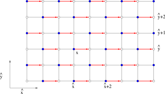
FIG. 2.: Checkerboard masking as seen in an $\hat{x}$–$\hat{y}$ plane of the lattice when using the standard Wilson action. The highlighted links with arrows can be updated simultaneously.

Let us consider, for example, all of the links in the $\hat{x}$-$\hat{y}$ plane which are oriented in the $\hat{x}$ direction. We can see from Fig. 2 that we can choose a “checkerboard” of such links that can be updated at the same time without interfering with each other. These links are indicated in the figure as highlighted links with arrows. It is easy to see that none of the links to be updated lie in any of the staples for the other links to be updated and that exactly half of the $\hat{x}$-oriented links in this plane can be simultaneously updated at one time.

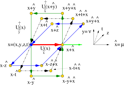
FIG. 3.: Rotating the $1\times{1}$ plaquette sitting in the $\hat{x}\hat{y}$ plane about the $\hat{x}$–axis into the $\hat{x}\hat{z}$ and $\hat{x}\hat{t}$ planes.

We have identified one of the lattice sites in Fig. 2 as the site $x$. If the the link variable $U_{\hat{x}}(x)$ is to updated then from Fig. 2, it is observed that the link variables in the $\hat{x}$ direction that can be simultaneously updated are $U_{\hat{x}}(x+2\hat{x})$, $U_{\hat{x}}(x+4\hat{x})$ and so on. So every second link along the $\hat{x}$ direction can be updated at the same time. Now let us consider stepping in the $\hat{y}$ direction. We again see that every second link in that direction can be simultaneously updated. By symmetry the same must also be true for the $\hat{z}$ and $\hat{t}$ directions as depicted in Fig. 3, where we have used a broken dash-dot line to try to indicate the fourth dimension (i.e., for the links that lie in the $\hat{x}$–$\hat{t}$ plane). We see that for the link pointing in the $\hat{x}$ direction, the plaquettes (and staples) in the $\hat{x}$–$\hat{y}$, $\hat{x}$–$\hat{z}$, $\hat{x}$–$\hat{t}$ planes are all related by simple rotations about the link. Thus we see that we have now built up a four-dimensional mask for determining which links pointing in the $\hat{x}$ direction can be simultaneously updated.

Let us introduce some convenient shorthand notation. If for a given link pointing in the direction $\mu$, we must take $n$ steps in the direction $\nu$ before reaching the next updatable link pointing in the direction $\mu$, we will use the notation $\mu:\nu\sim n\nu$. For our checkerboard masking we see that for a link pointing in the direction $\hat{x}$ we have to take two steps in each of the Cartesian directions before reaching the next updatable link. Hence we write

$$\hat{x}:\hskip 14.22636pt\hat{x}\sim{2\hat{x}}\hskip 7.11317pt{\rm,}\hskip 14.22636pt\hat{y}\sim{2\hat{y}}\hskip 7.11317pt{\rm,}\hskip 14.22636pt\hat{z}\sim{2\hat{z}} \hskip 7.11317pt{\rm and}\hskip 14.22636pt \hat{t}\sim{2\hat{t}}.$$ (7)

We immediately see that this is also true for links oriented in the $\hat{y}$, $\hat{z}$, and $\hat{t}$ directions so that

$$\hat{y}:\hskip 14.22636pt\hat{x}\sim{2\hat{x}}\hskip 7.11317pt{\rm,}\hskip 14.22636pt\hat{y}\sim{2\hat{y}}\hskip 7.11317pt{\rm,}\hskip 14.22636pt\hat{z}\sim{2\hat{z}} \hskip 7.11317pt{\rm and}\hskip 14.22636pt \hat{t}\sim{2\hat{t}},$$ (8)

$$\hat{z}:\hskip 14.22636pt\hat{x}\sim{2\hat{x}}\hskip 7.11317pt{\rm,}\hskip 14.22636pt\hat{y}\sim{2\hat{y}}\hskip 7.11317pt{\rm,}\hskip 14.22636pt\hat{z}\sim{2\hat{z}} \hskip 7.11317pt{\rm and}\hskip 14.22636pt \hat{t}\sim{2\hat{t}},$$ (9)

$$\hat{t}:\hskip 14.22636pt\hat{x}\sim{2\hat{x}}\hskip 7.11317pt{\rm,}\hskip 14.22636pt\hat{y}\sim{2\hat{y}}\hskip 7.11317pt{\rm,}\hskip 14.22636pt\hat{z}\sim{2\hat{z}} \hskip 7.11317pt{\rm and}\hskip 14.22636pt \hat{t}\sim{2\hat{t}}.$$ (10)

Finally, note that when we wish to update all of the links pointing in any one of the four Cartesian directions, say $\mu$, we need only two four-dimensional masks. This is because exactly half of the $\mu$-oriented links across the entire lattice are considered in each four-dimensional mask. To appreciate this we simply note that for any one of the Cartesian directions one mask can be turned into the checkerboard complement mask for that direction by shifting the mask by one step in any Cartesian direction, (see Fig. 2). So to update all of the links on the lattice we need a total of 8 four-dimensional masks, i.e., 2 masks for each of the four Cartesian directions. In other words, no matter how many nodes we have available on our parallel computing architecture a full lattice updating sweep will require 8 serial masked sweeps to complete with a nearest neighbour action (such as the Wilson action) and checkerboard masking. This is the conventional procedure for the standard Wilson action in lattice QCD studies. In closing this section on the standard Wilson action let us observe in Sec. III B that there is an alternative and equally good “linear” masking for this case.

B Linear Masking.

As an alternative approach to the checker board masking described in Sec. III A, one could partition the links over the lattice in a linear fashion as shown in Fig. 4.

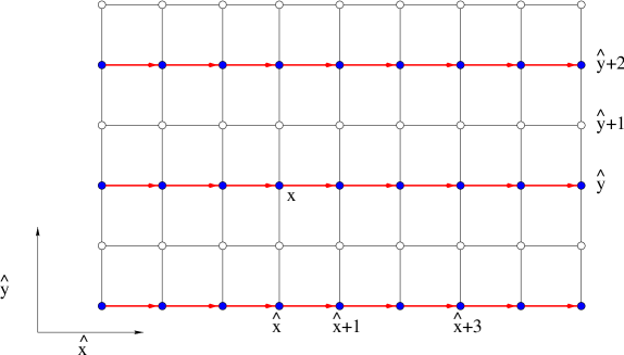
FIG. 4.: Linear masking of the lattice when using standard Wilson action. The highlighted arrows represents the link variable that can be updated simultaneously.

If the link variable of interest is $U_{\hat{x}}(x)$ then the next possible link variable in the $\hat{x}$ direction which can be updated is the $U_{\hat{x}}(x+\hat{x})$ link and then the $U_{\hat{x}}(x+2\hat{x})$ and so on. We see that all the links on the $\hat{x}$ line can be updated at the same time, since none of these links are contained in the $1\times 1$ plaquettes for the other links in the line. Hence we have $\hat{x}:\hat{x}\sim 1\hat{x}$. Now looking in the $\hat{y}$ direction, we realize that we cannot touch the $U_{\hat{x}}(x+\hat{y})$ link because it is part of the Wilson loop containing the link variable $U_{\hat{x}}(x)$ which is being updated simultaneously. However, the links $U_{\hat{x}}(x+2\hat{y})$, $U_{\hat{x}}(x+4\hat{y})$, etc. can be updated. Consequently, we have $\hat{x}:\hat{y}\sim{2\hat{y}}$ and similarly for steps in the $\hat{z}$ and $\hat{t}$ directions. For a link variable pointing in the $\hat{x}$ direction we then have that

$$\hat{x}:\hskip 14.22636pt\hat{x}\sim{1\hat{x}}\hskip 7.11317pt{\rm,}\hskip 14.22636pt\hat{y}\sim{2\hat{y}}\hskip 7.11317pt{\rm,}\hskip 14.22636pt\hat{z}\sim{2\hat{z}} \hskip 7.11317pt{\rm and}\hskip 14.22636pt \hat{t}\sim{2\hat{t}}.$$ (11)

When the links to be updated are pointing in the other three directions we have

$$\hat{y}:\hskip 14.22636pt\hat{x}\sim{2\hat{x}}\hskip 7.11317pt{\rm,}\hskip 14.22636pt\hat{y}\sim{1\hat{y}}\hskip 7.11317pt{\rm,}\hskip 14.22636pt\hat{z}\sim{2\hat{z}} \hskip 7.11317pt{\rm and}\hskip 14.22636pt \hat{t}\sim{2\hat{t}},$$ (12)

$$\hat{z}:\hskip 14.22636pt\hat{x}\sim{2\hat{x}}\hskip 7.11317pt{\rm,}\hskip 14.22636pt\hat{y}\sim{2\hat{y}}\hskip 7.11317pt{\rm,}\hskip 14.22636pt\hat{z}\sim{1\hat{z}} \hskip 7.11317pt{\rm and}\hskip 14.22636pt \hat{t}\sim{2\hat{t}},$$ (13)

$$\hat{t}:\hskip 14.22636pt\hat{x}\sim{2\hat{x}}\hskip 7.11317pt{\rm,}\hskip 14.22636pt\hat{y}\sim{2\hat{y}}\hskip 7.11317pt{\rm,}\hskip 14.22636pt\hat{z}\sim{2\hat{z}} \hskip 7.11317pt{\rm and}\hskip 14.22636pt \hat{t}\sim{1\hat{t}},$$ (14)

for the $\hat{y},\hat{z}$ and $\hat{t}$ directions respectively.

Again, we see that there are two complementary linear masks for links pointing in any given Cartesian direction $\mu$. One mask can be obtained from the other by a shift of one step in any of the three Cartesian directions orthogonal to $\mu$ as can be appreciated from Fig. 4. Thus this linear masking is equally as efficient as the checkerboard masking of the previous section, since there are 2 masks for each of the 4 Cartesian directions giving a total of 8 masks.

IV Masking an Improved Action.

In this section, we describe the necessary masking procedure for a first-level improved action involving $1\times 1$ and $1\times 2$ Wilson loops. In particular, in this section we are describing the masking suitable for the improved gauge action of Eq. (2), which has been used extensively by us [13, 14, 15, 16, 17]. Let us again begin by considering the link variable beginning at some lattice site $x$ and pointing in the $\hat{x}$ direction, i.e., $U_{\hat{x}}(x)$. We now need to consider both Fig. 3 for the elementary $1\times 1$ square plaquette and Fig. 5 for the $1\times 2$ rectangular plaquette. In Fig. 5 we show all of the $1\times 2$ rectangular plaquettes which contain the link $U_{\hat{x}}(x)$, which is shown as the highlighted horizontal link in the three parts of this figure. Visualizing a four dimensional object on a flat piece of paper can be, to a certain extent, an artistic challenge and so we have again used a dash–dot line to indicate links lying in the $\hat{x}$–$\hat{t}$ plane. There are three distinguishable ways to include this link in a $1\times 2$ plaquette (the three parts of the figure) and for each of these there are two (mirror-image) rectangles per Cartesian plane and four Cartesian planes. All links in Figs. 3 and 5 with arrows (other than the link $U_{\hat{x}}(x)$ itself) must be omitted from the mask when updating this link with our improved action. We see that there are many excluded links.

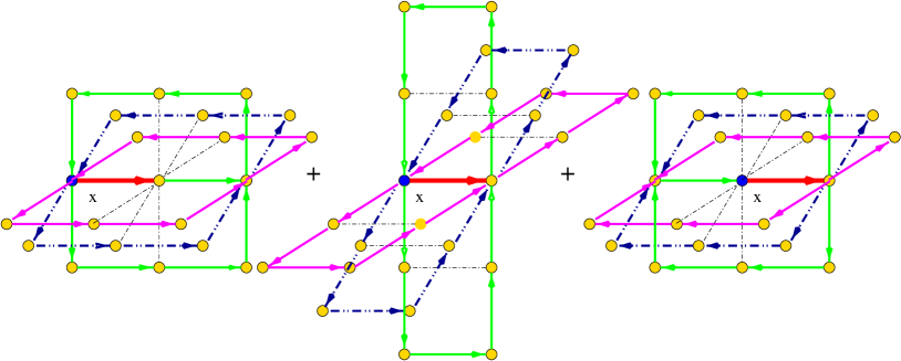
FIG. 5.: The set of all possible $1\times 2$ plaquettes containing the link $U_{\hat{x}}(x)$. The dashed-dotted line is to be understood as being in the $\hat{x}$–$\hat{t}$ plane.

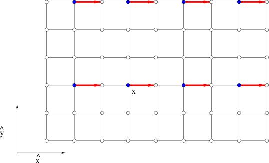
FIG. 6.: The highlighted links with arrows are the ones that can be simultaneously updated for an action containing both $1\times 1$ and $1\times 2$ plaquettes.

In Fig. 6 we show which links can be simultaneously updated with the link $U_{\hat{x}}(x)$. We can immediately write down by inspection from this figure that

$$\hat{x}:\hskip 14.22636pt\hat{x}\sim{2\hat{x}}\hskip 7.11317pt{\rm,}\hskip 14.22636pt\hat{y}\sim{3\hat{y}}\hskip 7.11317pt{\rm,}\hskip 14.22636pt\hat{z}\sim{3\hat{z}} \hskip 7.11317pt{\rm and}\hskip 14.22636pt \hat{t}\sim{3\hat{t}}\,.$$ (15)

This follows since the $\hat{z}$ and $\hat{t}$ cases are identical to the $\hat{y}$ case for this $\hat{x}$–oriented link. The generalization to the other orientations of the links to be updated is straightforward by symmetry

$$\hat{y}:\hskip 14.22636pt\hat{x}\sim{3\hat{x}}\hskip 7.11317pt{\rm,}\hskip 14.22636pt\hat{y}\sim{2\hat{y}}\hskip 7.11317pt{\rm,}\hskip 14.22636pt\hat{z}\sim{3\hat{z}} \hskip 7.11317pt{\rm and}\hskip 14.22636pt \hat{t}\sim{3\hat{t}},$$ (16)

$$\hat{z}:\hskip 14.22636pt\hat{x}\sim{3\hat{x}}\hskip 7.11317pt{\rm,}\hskip 14.22636pt\hat{y}\sim{3\hat{y}}\hskip 7.11317pt{\rm,}\hskip 14.22636pt\hat{z}\sim{2\hat{z}} \hskip 7.11317pt{\rm and}\hskip 14.22636pt \hat{t}\sim{3\hat{t}},$$ (17)

$$\hat{t}:\hskip 14.22636pt\hat{x}\sim{3\hat{x}}\hskip 7.11317pt{\rm,}\hskip 14.22636pt\hat{y}\sim{3\hat{y}}\hskip 7.11317pt{\rm,}\hskip 14.22636pt\hat{z}\sim{3\hat{z}} \hskip 7.11317pt{\rm and}\hskip 14.22636pt \hat{t}\sim{2\hat{t}}\,.$$ (18)

Let us return to the particular case of the masking for $\hat{x}$-oriented links. From Eq. (15) we see that there is symmetry between the $\hat{y}$, $\hat{z}$, and $\hat{t}$ directions and so we will begin by constructing suitable masks for any given equal-$x$ hyper-plane, i.e., for the three dimensional space spanned by the unit vectors $\hat{y}$, $\hat{z}$, and $\hat{t}$.

Before attempting this, let us first consider Fig. 6 and extend this to three dimensions by imagining that the $\hat{z}$-axis is pointing directly out from the page. We shall temporarily neglect the $\hat{t}$ direction, which is equivalent to simply taking a slice of the four-dimensional lattice with the same value of $t$, (i.e., an equal-$t$ hyper-plane). Now let us view this three-dimensional lattice by looking along the $\hat{x}$-axis at one particular equal-$x$ plane. We will then be presented with end-views of updatable links in the $\hat{y}$–$\hat{z}$ plane. For every fixed value of $z$ there are three different masks needed for $y$ and vice versa. Also, there is no restriction on simultaneously updating diagonally shifted links, since we are only considering planar actions at this point. It is not difficult to see that we can cover all of the nine lattice links that need to be updated with three orthogonal masks as shown in Fig. 7. In this figure $x$-oriented links which can be updated at the same time are indicated by a solid dot. Note that each of these masks is related by a diagonal shift of the nine-point lattice “window”.

FIG. 7.: Schematic illustration of the lattice masking when using the $1\times 2$ plaquette improved action.

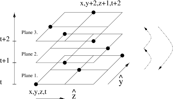
FIG. 8.: Illustration of the cyclic plane rotation in the improved masking.

We can now also extend this thinking to include the $t$ direction, by stacking the three two-dimensional $y$–$z$ masks on top of each other as shown in Fig. 8. We must stack the planes so that when viewed along any of the three axes the solid dots in any one Cartesian planes always have the appearance of one of the planes in Fig. 7. We see that this can be achieved in three ways by the stacking in Fig. 8 and its two cyclic permutations. These three three-dimensional masks when summed give the identity (i.e., the sum includes all points) and are orthogonal to each other (i.e., the sum includes all points only once).

We can now give a simple geometrical picture of what we are doing, which will simplify the generalization that we give in the next section. For $\hat{x}$-oriented links, the directions $\hat{y}$, $\hat{z}$, and $\hat{t}$ directions are all symmetrical and each direction requires a step of 3 to reach the next updatable link. Hence, we need to construct a complete set of orthogonal masks in three dimensions for a $3\times 3\times 3$ cube, where no two points in the cube lie on the same Cartesian axis (i.e., only diagonally related points). This is simple to do. Let us consider the bottom plane (i.e., plane 1) of Fig. 8 and connect the three solid dots by a diagonal line. We see that plane 2 is obtained from plane 1 by a diagonal shift of this line by one diagonal half-step, and similarly for plane 3. In visualizing this it may help to imagine surrounding the cube by many identical copies of itself and moving the diagonal line through diagonal half-steps across all of these cubes simultaneously. All three three-dimensional masks are obtained in the same way but start with plane 1, plane 2, and plane 3 respectively.

So for the $\hat{x}$-oriented links we need 3 masks for each equal-$x$ hyper-plane (i.e., a three-volume here) and we have two independent equal-$x$ hyper-planes, giving a total of 6 masks for each Cartesian direction for the link orientation. Since there are 4 orientations, then there is a total of 24 masks needed for an action containing both $1\times 1$ and $1\times 2$ plaquettes. Thus a single lattice sweep must take at least 24 sequential serial calculations even on the most parallel computing architecture.

The masking procedure outlined here for this action can only be implemented when the number of lattice points in each dimension is a multiple of three. Inspection of Fig. 8 reveals the periodicity of three is required to maintain separation of links at the boundary. Since simulations are usually carried out on lattices with even numbered sides, this restricts the length of the lattice sides to multiples of six. Fortunately, multiples of four are easily obtained as described in the next section. Moreover, Sec. VI reports a high-performance mask for this action with a periodicity of four.

It is interesting to note that when implementing this masking procedure on the CM-5 we achieved optimum performance by calculating the updates for all links on the lattice and by then only implementing those updates that were appropriate for the particular mask being used at the time. In other words for the lattices that we have studied so far on the CM-5 it was more efficient to calculate link updates that were never used, than it was to split the masked links over the various processor nodes and update only these masked links. This was due to the fact that there was a large overhead of communication time in assigning the masked links across the processors. The point of this observation is that the optimal use of the masks will in general depend on the details of the parallel computing architecture being used.

V Masking the Lattice When Using a Generalized Improved Action.

We can now generalize the algorithm presented in Sec. IV for arbitrarily improved planar actions. Let us begin as before by considering the update of links oriented in the $\hat{x}$-direction. Let us assume that we have an action with $n\times m$ links where the $n$ refers to the $\hat{x}$ direction and the $m$ refers to the $\hat{y}$, $\hat{z}$, $\hat{t}$ directions. We will eventually argue that only the $n_{\rm max}\times n_{\rm max}$ case, where $n_{\rm max}$ is the greater of $n$ and $m$, is necessary in the general case. As shown in Fig. 9 the nearest simultaneously updatable links are separated by $n$ steps in the $\hat{x}$ direction and $(m+1)$ steps in the other three Cartesian directions.

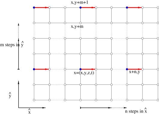
FIG. 9.: The highlighted links with arrows are the ones that can be simultaneously updated for an action containing up to $n\times m$ plaquettes, where here $n$ refers to the $\hat{x}$ direction and $m$ applies to the other three Cartesian directions.

Hence we see that we can write in our notation for the four Cartesian orientations of the links that

$$\hat{x}:\hskip 14.22636pt\hat{x}\sim{n\hat{x}}\hskip 7.11317pt{\rm,}\hskip 14.22636pt\hat{y}\sim{(m+1)\hat{y}}\hskip 7.11317pt{\rm,}\hskip 14.22636pt\hat{z}\sim{(m+1)\hat{z}}\hskip 7.11317pt{\rm and}\hskip 14.22636pt\hat{t}\sim{(m+1)\hat{t}},$$ (19)

$$\hat{y}:\hskip 14.22636pt\hat{x}\sim{(m+1)\hat{x}}\hskip 7.11317pt{\rm,}\hskip 14.22636pt\hat{y}\sim{n\hat{y}}\hskip 7.11317pt{\rm,}\hskip 14.22636pt\hat{z}\sim{(m+1)\hat{z}}\hskip 7.11317pt{\rm and}\hskip 14.22636pt\hat{t}\sim{(m+1)\hat{t}},$$ (20)

$$\hat{z}:\hskip 14.22636pt\hat{x}\sim{(m+1)\hat{x}}\hskip 7.11317pt{\rm,}\hskip 14.22636pt\hat{y}\sim{(m+1)\hat{y}}\hskip 7.11317pt{\rm,}\hskip 14.22636pt\hat{z}\sim{n\hat{z}}\hskip 7.11317pt{\rm and}\hskip 14.22636pt\hat{t}\sim{(m+1)\hat{t}},$$ (21)

$$\hat{t}:\hskip 14.22636pt\hat{x}\sim{(m+1)\hat{x}}\hskip 7.11317pt{\rm,}\hskip 14.22636pt\hat{y}\sim{(m+1)\hat{y}}\hskip 7.11317pt{\rm,}\hskip 14.22636pt\hat{z}\sim{(m+1)\hat{z}}\hskip 7.11317pt{\rm and}\hskip 14.22636pt\hat{t}\sim{n\hat{t}}\,.$$ (22)

We can now follow the arguments of the previous section. Let us consider a fixed-$x$ hyper-plane (i.e., three-volume). In place of a $3\times 3$ three-volume we will now need an $(m+1)\times(m+1)\times(m+1)$ three-volume. Furthermore, we will need a complete set of orthogonal and diagonal masks for this. Let us again look along the $\hat{x}$ direction at a fixed $t$ plane for now, i.e., we are looking at a $\hat{y}$–$\hat{z}$ plane as in Fig. 10. Let us refer to the $(m+1)\times(m+1)$ two-dimensional plane with the updatable links (solid dots) along the diagonal as plane 1. Then we can generate the other $m$ two-dimensional planes by diagonal half-shifts as before as depicted in Figs. 11 and 12. We can then sequentially stack these planes in the $\hat{t}$ direction as before to form the first of the three-dimensional masks. The other $m$ three-dimensional masks are then generated from this first mask by the cyclic permutations of the $m+1$ planes as in Sec. IV. Hence we have generated the desired complete set of $(m+1)$ orthogonal three-dimensional diagonal masks.

FIG. 10.: Plane 1 with the $(m+1)$ updatable sites on the main diagonal of the $\hat{y},\hat{z}$ plane.

FIG. 11.: Plane 2.

FIG. 12.: Plane 3.

So for each fixed $x$-hyper-plane (i.e., three volume) we need $(m+1)$ masks. We will need such a set of masks for the $n$ values of $x$. The general result is that for updating the links oriented in the $\hat{x}$ direction we need a total of $n\times(m+1)$ masks and we have seen that the construction of these masks is straightforward. The construction of the masks for the other Cartesian orientations of the links proceeds identically. This total number of masks is $n_{\rm mask}=4\times n\times(m+1)$. The periodicity of the mask is governed by the last factor, $(m+1)$, and the lengths of the lattice dimensions must be a multiple of this number. The reason for this is that if this were not the case then the imposition of the necessary periodic boundary conditions would cause link collisions, where a link being updated uses one or more other links which are simultaneously being updated.

Any improved lattice action of physical interest must be both $Z_{4}$-symmetric (i.e., symmetric under the arbitrary interchange of the four Cartesian directions) and translationally invariant. Thus for such actions every link will find itself occurring in every possible position for every plaquette in the improved action. We then see, as we did in Sec. IV and Fig. 5, that the number of steps needed in each direction is determined by the longest plaquette side appearing in the action. Let us denote the longest plaquette side appearing in the action as $n_{\rm max}$. Then we see that the number of steps needed in the various Cartesian directions is given by

$$\hat{x}:\hskip 14.22636pt\hat{x}\sim{n_{\rm max}\hat{x}}\hskip 7.11317pt{\rm,}\hskip 14.22636pt\hat{y}\sim{(n_{\rm max}+1)\hat{y}}\hskip 7.11317pt{\rm,}\hskip 14.22636pt\hat{z}\sim{(n_{\rm max}+1)\hat{z}}\hskip 7.11317pt{\rm and}\hskip 14.22636pt\hat{t}\sim{(n_{\rm max}+1)\hat{t}},$$ (23)

$$\hat{y}:\hskip 14.22636pt\hat{x}\sim{(n_{\rm max}+1)\hat{x}}\hskip 7.11317pt{\rm,}\hskip 14.22636pt\hat{y}\sim{n_{\rm max}\hat{y}}\hskip 7.11317pt{\rm,}\hskip 14.22636pt\hat{z}\sim{(n_{\rm max}+1)\hat{z}}\hskip 7.11317pt{\rm and}\hskip 14.22636pt\hat{t}\sim{(n_{\rm max}+1)\hat{t}},$$ (24)

$$\hat{z}:\hskip 14.22636pt\hat{x}\sim{(n_{\rm max}+1)\hat{x}}\hskip 7.11317pt{\rm,}\hskip 14.22636pt\hat{y}\sim{(n_{\rm max}+1)\hat{y}}\hskip 7.11317pt{\rm,}\hskip 14.22636pt\hat{z}\sim{n_{\rm max}\hat{z}}\hskip 7.11317pt{\rm and}\hskip 14.22636pt\hat{t}\sim{(n_{\rm max}+1)\hat{t}},$$ (25)

$$\hat{t}:\hskip 14.22636pt\hat{x}\sim{(n_{\rm max}+1)\hat{x}}\hskip 7.11317pt{\rm,}\hskip 14.22636pt\hat{y}\sim{(n_{\rm max}+1)\hat{y}}\hskip 7.11317pt{\rm,}\hskip 14.22636pt\hat{z}\sim{(n_{\rm max}+1)\hat{z}}\hskip 7.11317pt{\rm and}\hskip 14.22636pt\hat{t}\sim{n_{\rm max}\hat{t}}\,.$$ (26)

Hence the number of masks in general for an improved action will then be given by

$$n_{\rm mask}=4\times n_{\rm max}\times(n_{\rm max}+1)$$ (27)

and the lattice will need the length in each dimension to be an integral multiple of $(n_{\rm max}+1)$.

It is useful to note that the linear masking for the standard Wilson action is the one that is extended initially in Sec. IV and is subsequently generalized in this section. For the standard Wilson action (i.e., $1\times 1$ plaquettes only) we see that $n_{\rm max}=1$ and hence $n_{\rm mask}=4\times 1\times 2=8$ as we found for the linear (and checkerboard) mask. For the improved action that we have studied (i.e., $1\times 1$ and $1\times 2$ plaquettes) we have $n_{\rm max}=2$ and hence $n_{\rm mask}=4\times 2\times 3=24$ or 6 masks per link direction as found in Sec. IV. However, this way of proceeding for the plaquette plus rectangle improved action would require each lattice dimension be a multiple of $(n_{\rm max}+1)=3$, but since we also typically want our lattices to have even lengths then that means each side of the lattice would need to be a multiple of 6 in length. Since the result in Eq. (27) is a lower bound, we can of course always choose to enlarge the period of our masking by choosing $n_{\rm max}+2$ for the last factor in Eq. 27 rather than $n_{\rm max}+1$. This will still ensure that no link collisions occur. For example, for the plaquette plus rectangle improved action we can use $(n_{\rm max}+2)=4$ instead of $(n_{\rm max}+1)=3$ in Eq. (27), so that any lattice lengths which are multiples of 4 become available at the cost of requiring 32 masks rather than 24. Fortunately, for this case a more efficient mask can be realized and will be presented in the next section.

VI Non-planar Considerations

We have presented a method for identifying links which may be simultaneously updated during Monte-Carlo updates or cooling sweeps. The generality of the algorithm allows one to parallelize link updates for planar actions of any degree of non locality. In this section we extend this analysis to a few special cases of actions in which out-of-plane considerations are necessary. Both cases are centred around the plaquette plus rectangle action of Eq. (2) in which $1\times 1$ and $1\times 2$ Wilson loops are considered in the action. Such actions dominate current improved gauge action analyses.

In Sec. IV we illustrated how such an action can be masked through the consideration of an elementary $3\times 3\times 3$ cube in which one-third of the links may be simultaneously updated. However, only every second link in the direction of the links is updated simultaneously as illustrated in Fig. 6. Hence six masks per link direction are required.

Here we consider an alternative masking specialized to the $1\times 1$ and $1\times 2$ Wilson loop actions. Fig. 13 illustrates the manner in which these Wilson loops may be nested, such that one need not restrict the mask to every second link in the direction of the links being updated. This technique will reduce the number of masks by a factor of two, at the expense of considering an elementary $4\times 4\times 4$ cube in which one-quarter of the links may be simultaneously updated. Fig. 14 displays the four planes to be cycled through in which the links to be updated simultaneously are indicated by the solid dot. Hence only four masks per link direction are required. Moreover, the lattice dimensions (usually even numbers) can now be multiples of four as opposed to six.

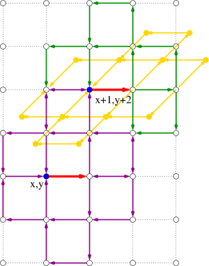
FIG. 13.: Two elementary cells for an action involving $1\times 1$ and $1\times 2$ Wilson loops are nested together such that one need not restrict the mask to every second link in the direction of the links being updated. The links with the positions labeled are the ones that can be simultaneously updated. The out of plane plaquette-plus-rectangle illustrates additional links that cannot be simultaneously updated.

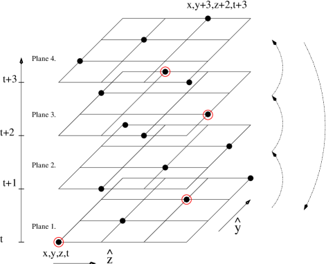
FIG. 14.: The four planes to be cycled through in the elementary $4\times 4\times 4$ cube. One-quarter of the links may be updated simultaneously and are indicated by the solid dot. The circled sites are an example of the sites surviving when the out of plane “chair” or “parallelogram” link paths are included in the action.

The out-of-plane considerations required for the nested action are also indicated in Fig. 13. Hence it becomes apparent that not only the three links at $(x,y+1)$, $(x,y+2)$, and $(x,y+3)$, be avoided, but also the links two-steps in a direction orthogonal to the link direction and one step in a third direction (similar to moves of a Knight on a chess board) must be avoided.

Inspection of the four planes to be cycled through in the elementary $4\times 4\times 4$ cube displayed in Fig. 14 indicates that such Knight moves are already avoided in this mask. However, it also becomes clear that the ordering of the planes is crucial. For example interchanging the positions of planes 2 and 3 would cause “link collisions” within the nested mask.

Finally we consider non-planar actions in which one step out of the plane of the $1\times 1$ and $1\times 2$ Wilson loops is required. Such non-planar paths are introduced to eliminate small but finite ${\cal O}(g^{2}a^{2})$ errors where $g$ is the gauge coupling constant. The six-link paths commonly referred to as the “chair” and “parallelogram” [18] introduce a link parallel to that being updated which is one-step orthogonal to the link direction and one step in a third direction.

Inspection of Fig. 14 indicates that such 1 by 1 moves eliminates fully two of the four planes and half of the parallel sites on each surviving plane. An example of four of the sites which may still be updated in parallel are indicated by the circled sites in Fig. 14. As a result there are now 16 masks required per link direction instead of 4. Now a total of 64 masks is required for this action which is still regarded as rather local.

The introduction of even the most local non-planar paths can have a serious detrimental effect on the level of parallelism that is possible. It is easy to see that one can rapidly eliminate all sites in an elementary $n\times n\times n$ cube with non-planar loops, leading to $n^{3}$ masks per link direction.

VII Summary and Conclusion

We have briefly described the concept of improved actions and have explained the implications of the non locality arising from the improvement program for the implementation of these actions on parallel computing architectures. We have characterized these implications in terms of the number of masks, which in turn determine the minimum number of serial calculations needed to perform a Monte Carlo updating sweep over all of the gluon links on the lattice. We have systematically built up a completely general algorithm using masks that allow one to put any planar improved lattice action on a parallel machine in an efficient way. The generalized masking construction are given in Sec. V.

Non-planar considerations encountered in nesting specific planar actions and actions involving non-planar loops have also been addressed. We hope that the methodology presented will allow one to find an efficient parallel mask for any desired action. We are currently testing our algorithms on some highly improved actions and will be reporting the results of these studies[17] in the near future.

VIII Acknowledgment.

This research was supported by the Australian Research Council and by grants of supercomputer time on the CM-5 made available through the South Australian Centre for Parallel Computing. AGW also acknowledges support from the U.S. Department of Energy Contract No. DE-FG05-86ER40273 and by the Florida State University Supercomputer Computations Research Institute which is partially funded by the Department of Energy through Contract No. DE-FC05-85ER2500.

REFERENCES

- [1] M.E. Peskin and D.V. Schroeder, ”An Introduction to Quantum Field Theory,” (Addison-Wesley, New York, 1995) 842 pp.
- [2] T. Muta, ”Foundations Of Quantum Chromodynamics: An Introduction To Perturbative Methods In Gauge Theories,” Singapore: World Scientific (1987) 409 pp., (World Scientific Lecture Notes In Physics, 5).
- [3] H.J. Rothe, ”Lattice gauge theories: An Introduction”, (World Scientific, Singapore, 1992) 381pp.
- [4] I. Montvay and G. Munster, ”Quantum Fields on a Lattice”, (Cambridge University Press, Cambridge UK, 1994) 491 pp., (Cambridge monographs on mathematical physics).
- [5] D. Schutte, W. Zheng and C. J. Hamer, Phys. Rev. D55, 2974 (1997) [hep-lat/9603026].
- [6] Stanley J. Brodsky and Hans-Christian Pauli and Stephen S. Pinsky, Phys. Rept. bf 301, 299-486 (1998). bf hep-ph/9705477; Stanley J. Brodsky and Gary McCartor and Hans Christian Pauli and Stephen S. Pinsky, Part. World bf Vol 3, 109-124, (1993); Stanislaw Glazek and Avaroth Harindranath and Stephen Pinsky and Junko Shigemitsu and Kenneth Wilson, Phys. Rev. D47, 1599 (1993).
- [7] Craig D. Roberts and Anthony G. Williams, Prog. Part. Nucl. Phys. bf Vol 33, 477-575 (1994). bf hep-ph/9403224.
- [8] Lattice 99, Nucl. Phys. (Proc. Suppl.) 83, (2000).
- [9] G.P. Lepage and D.B. Mackenzie, Phys. Rev. D 48, 2250 (1993), hep-lat/9209022.
- [10] G.P. Lepage,“Redesigning lattice QCD”, hep-lat/9607076.
- [11] K.G. Wilson, Phys. Rev. D 10, 2445 (1974).
- [12] H.R. Fiebig and R.M. Woloshyn, Nucl. Phys. B53, (Proc. Suppl.), 886 (1997), hep-lat/9607058.
- [13] F.D.R. Bonnet, P. Fitzhenry, D.B. Leinweber, M. Standford, and A.G. Williams, submitted for publication.
- [14] F.D.R. Bonnet, P.O. Bowman, D.B. Leinweber, D.G. Richards, A.G. Williams, Aust. J. Phys. 52, 939 (1999), hep-lat/9905006.
- [15] F.D.R. Bonnet, D.B. Leinweber, A.G. Williams, and J.M. Zanotti, hep-lat/9912044.
- [16] F.D.R. Bonnet, P.O. Bowman, D.B. Leinweber, and A.G. Williams, in preparation.
- [17] S. Bilson-Thompson, F.D.R. Bonnet, D.B. Leinweber, and A.G. Williams, in preparation.
- [18] M. Alford, W. Dimm, and P. Lepage, Phys. Lett. B361, 87 (1995).
- [19] F.X. Lee and D.B. Leinweber, Phys. Rev. D 59, 074504 (1999), hep-lat/9711044.
- [20] H.R. Fiebig and R.M. Woloshyn, Phys. Lett. B385, 273 (1996), hep-lat/9603001.
- [21] N. Cabibbo and E. Marinari, Phys. Lett. B119, 387 (1982).