Measurement of the inclusive differential cross section for $Z$ bosons as a function of transverse momentum in $\overline{p}p$ collisions at $\sqrt{s}=1.8$ TeV

Abstract

We present a measurement of the differential cross section as a function of transverse momentum of the $Z$ boson in $p\overline{p}$ collisions at $\sqrt{s}=1.8$ TeV using data collected by the DØ experiment at the Fermilab Tevatron Collider during 1994–1996. We find good agreement between our data and the NNLO resummation prediction and extract values of the non-perturbative parameters for the resummed prediction from a fit to the differential cross section.

I Introduction

The study of the production properties of the $Z$ boson began in 1983 with its discovery by the UA1 and UA2 collaborations at the CERN $p\overline{p}$ collider [1, 2]. Together with the discovery of the $W$ boson [3, 4] earlier that year, the observation of the $Z$ boson provided a direct confirmation of the unified model of the weak and electromagnetic interactions, which, together with QCD, is now called the standard model. Since its discovery, many of the intrinsic properties of the $Z$ boson have been examined in great detail via $e^{+}e^{-}$ collisions at the LEP $e^{+}e^{-}$ collider at CERN  [5]. The mass of the $Z$ boson measured at LEP and the SLC $e^{+}e^{-}$ collider at SLAC, known to better than one part in $10^{4}$ [6], is one of the most precisely measured parameters in particle physics.

LEP experiments have focused on the intrinsic properties of the $Z$ boson, examining the electroweak character of its production and decay in $e^{+}e^{-}$ collisions. At the Tevatron, where the $Z$ boson is produced in $p\overline{p}$ collisions, its production properties are presumably characterized by QCD. Since the electroweak properties of the $Z$ boson are not correlated with the strong properties of its production, the $Z$ boson can therefore serve as a clean probe of the strong interaction. Also, the large mass of the $Z$ boson assures a large energy scale ($Q^{2}\approx M_{Z}^{2})$ for probing perturbative QCD with good reliability. The measurement of the cross section as a function of transverse momentum ($d\sigma/dp_{T}$) of the $Z$ boson provides a sensitive test of QCD at high-$Q^{2}$. In this article, we describe a measurement of $d\sigma/dp_{T}$ of the $Z$ boson using the $e^{+}e^{-}$  decays of the $Z$ [7].

In the parton model, at lowest order, $Z$ bosons are produced in head-on collisions of $q\overline{q}$ constituents of the proton and antiproton, and cannot have any transverse momentum. Consequently, the fact that observed $Z$ bosons have finite $p_{T}$ is attributed to gluon radiation from the colliding partons prior to their annihilation into the $Z$ boson. Gluon radiation within the color field of the proton or antiproton increases in proportion to the time available for such annihilation, which is proportional to the inverse of the energy scale for the process ($1/Q$) [8]. The radiated gluons carry away transverse momentum from the annihilating quarks and momentum conservation requires that this be observed in the $p_{T}$ of the $Z$ boson. Thus, one expects that the observed transverse momentum distribution of any dielectron system (produced at a scale $Q\approx M_{ee}$) will broaden as a function of $Q$. This is, indeed, the effect observed. At $M_{ee}\approx 10$ GeV, the typical $p_{T}$ for Drell-Yan pairs[9] is about 1 GeV[10]. For $W$ boson production ($Q\approx 80$ GeV), the average $p_{T}$ is about 5 GeV[11]. For $Z$ boson production ($Q\approx 91$ GeV), the average $p_{T}$ is about 6 GeV[12].

In general, the differential cross section for producing the state $V$ is given by:

$${d^{2}\sigma_{ij\rightarrow V}\over dp_{T}^{2}dy}=\sum_{i,j}\int dx_{i}dx_{j}f(x_{i})f(x_{j}){d^{2}\hat{\sigma}_{ij\rightarrow V}\over dp_{T}^{2}dy}$$ (1)

where $p_{T}$ and $y$ are the transverse momentum and the rapidity of the state $V$; $x_{i}$ and $x_{j}$ are the momentum fractions of the colliding partons; $f(x_{i})$ and $f(x_{j})$ are the parton distribution functions (pdf’s) for the incoming partons; and $\hat{\sigma}_{ij\rightarrow V}$ is the partonic cross section for production of the state V, in our case, the $Z$ boson. The subscripts $i$ and $j$ denote the contributing parton flavors (i.e., up, down, etc.) and the sum is over all such flavors.

In standard perturbative QCD (pQCD), one calculates the partonic cross section by expanding in powers of the strong coupling constant, $\alpha_{s}$. This procedure works well when $p_{T}^{2}\sim Q^{2}$. However, as $p_{T}\rightarrow 0$, correction terms that are proportional to $\alpha_{s}\ln(Q^{2}/{p_{T}^{2}})$ become significant for all values of $\alpha_{s}$, and the cross section diverges at small $p_{T}$. Physically, the failure of the calculation is due to the presence of collinear and low-$p_{T}$ gluons that are not properly accounted for in the standard perturbative expansion. This difficulty is surmounted by reordering the perturbative series through a technique called resummation [8, 13, 14, 15, 16, 17, 18, 19].

In its final form, the differential cross section is calculated as a Fourier transform in impact parameter, $b$, space:

$${d^{2}\sigma_{ij\rightarrow V}\over d{p_{T}^{2}}dy}\approx\int_{0}^{\infty}d^{2}b\ e^{i\vec{p}_{T}\cdot\vec{b}}W(b,Q)+Y(b,Q)$$ (2)

where $W(b,Q)$ contains the results of resumming the perturbative series, and $Y(b,Q)$ adds back to the calculation the pieces that are perturbative in $\alpha_{s}$, but are not singular at $p_{T}=0$[8].

Although the resummation technique extends the applicability of pQCD to lower values of $p_{T}$, a more fundamental barrier is encountered when $p_{T}$ approaches $\Lambda_{\text{Q}CD}$, and pQCD is expected to fail in general. In this region, we expect non-perturbative aspects of the strong force to dominate the production of the vector boson. This implies that $W(b,Q^{2})$ in Eq. 2 is undefined above some value of $b=b_{max}$. To extend the calculation to $p_{T}=0$, the following substitution is made:

$$W(b,Q)\rightarrow W(b_{*},Q)e^{-S_{NP}(b,Q)}$$ (3)

where $b_{*}\equiv b/\sqrt{1+(b/b_{\rm max})^{2}}$. This effectively cuts off the contribution of $W(b,Q)$ near $b_{\rm max}$, leaving the differential cross section dominated by $S_{NP}$, where $S_{NP}(b,Q)$ is called the non-perturbative Sudakov form factor. $S_{NP}$ has the generic renormalization group invariant form[8]

$$S_{NP}(b,Q)=$$ (4)

$$h_{1}(b,x_{i})+h_{1}(b,x_{j})+h_{2}(b)\cdot\ln({Q\over 2Q_{o}})$$ (5)

where $x_{i}$ and $x_{j}$ are the momentum fractions of the annihilating quarks; $Q_{o}$ is an arbitrary momentum scale; and $h_{1}(b,x)$, $h_{2}(b)$ are phenomenological functions to be determined from experiment[15, 17, 18]. The fact that $h_{2}(b)$ lacks any dependence on the momentum fractions of the incoming partons has led to speculation that it may contain some deeper relevance to the gluonic structure of the proton[20].

The current understanding of the $p_{T}$ distribution for $Z$ bosons uses fixed-order perturbative calculations [leading-order (LO) or next-to-leading-order (NLO)] to describe the high-$p_{T}$ region, and resummation calculations of the perturbative solution to describe the low-$p_{T}$ region. The resummation calculation fails at large-$p_{T}$ (of the order 50 GeV) due to large terms missing from the calculation resulting from the $p_{T}\rightarrow 0$ approximation. An ad hoc “matching” criteria is invoked to decide when to switch from the resummed calculation to the fixed-order calculation, which is considered to be robust at large-$p_{T}$. Additionally, a parameterization of Eq. 4 is invoked to account for non-perturbative effects at the lowest $p_{T}$ values which are not calculable in perturbative QCD.

In our measurement of the $p_{T}$ distribution, we restrict the invariant mass of the dielectron system to be approximately the mass of the $Z$ boson, where the $Z$ resonance greatly dominates dielectron production. The remaining contribution is due almost entirely to production of $e^{+}e^{-}$ pairs via the photon propagator (Drell-Yan process), which is coherent and interferes quantum mechanically with $Z$ boson production. Other processes also contribute to inclusive dielectron production in $p\overline{p}$ collisions, e.g., $t\overline{t}$ and diboson production, however, these are incoherent with $Z$ boson production and their overall rate is negligibly small.

Besides being of intrinsic interest in the study of QCD, precise understanding of $Z$ boson production in $p\overline{p}$ collisions has important practical benefits for other measurements with electrons in the final state. The phenomenology used to describe $Z$ boson production is applicable to $W$, $Z$, and essentially all Drell-Yan type processes. In the low-$p_{T}$ region, where the cross section is highest, uncertainties in the phenomenology of vector boson production have contributed to the uncertainty in the measurement of the mass of the $W$ boson ($M_{W}$) [21, 22]. Additionally, diboson, top quark, and Higgs boson production all have single and dielectron backgrounds from $W$ and $Z$ boson production that will be more constrained through a precise measurement of $Z$ boson production properties.

Despite larger statistical uncertainties relative to $W$ boson production (there are $\sim$10 times more $W\rightarrow e\nu$ than $Z\rightarrow ee$ events produced at $\sqrt{s}=1.8$ TeV), the $Z$ boson provides a better laboratory for evaluating the phenomenology of vector boson production. The measurement of the transverse momentum of the $e^{+}e^{-}$ pair ($p_{T}^{ee}$) does not suffer from the same level of experimental imprecision as the measurement of $p_{T}^{e\nu}$ because the latter relies on the determination of the total missing transverse momentum in the detector (${\hbox{$E$\kern-6.00006pt\lower-0.43057pt\hbox{/}}}_{T}$), which has inherently higher systematic uncertainties. The typical resolution in $p_{T}^{ee}$ is about 1.5 GeV compared with 4–5 GeV for $p_{T}^{e\nu}$, and the $p_{T}^{ee}$ resolution is approximately flat as $p_{T}^{ee}$ increases, whereas it continues to degrade for $p_{T}^{e\nu}$.

Previous measurements of the differential cross section for $Z\rightarrow ee$ production in $p\overline{p}$ collisions have been limited primarily by statistics. The UA2 [23] collaboration analyzed 162 events, concluding that there was basic agreement with QCD, but that more statistics were needed. In the 1988–89 run at the Tevatron, CDF [12] analyzed 235 dielectron events and 103 dimuon events, making similar conclusions. Our study is based on a total of about 6400 events. We determine the $p_{T}$ distribution for the $Z$ boson and use our results to constrain the non-perturbative Sudakov form factor. We then remove the effects of detector smearing and obtain a normalized differential cross section $d\sigma/dp_{T}$.

We present a brief description of the DØ detector in the next section. We then present the selection procedure for our data sample. The selection efficiency (Section  IV), kinematic and fiducial acceptances (Section  V), contributing backgrounds (Section  VI), fit for non-perturbative parameters (Section VIII), and the smearing correction (Section IX) are all discussed in turn. These individual components are combined (Section  X) to obtain the final differential cross section, which is compared to predictions from QCD.

II Experimental Setup

The DØ detector consists of three major subsystems: a central detector, a calorimeter (Fig. 1), and a muon spectrometer. It is discussed in detail elsewhere [24]. We describe below only the features that are most relevant for this measurement.

A Conventions

We use a right-handed Cartesian coordinate system with the $z$-axis defined by the direction of the proton beam, the $x$-axis pointing radially out of the Tevatron ring, and the $y$-axis pointing up. A vector $\vec{p}$ is then defined in terms of its projections on these three axes, $p_{x}$, $p_{y}$, $p_{z}$. Since protons and antiprotons in the Tevatron are unpolarized, all physical processes are invariant with respect to rotations around the beam direction. It is therefore convenient to use a cylindrical coordinate system, in which the same vector is given by the magnitude of its component transverse to the beam direction, $p_{T}$, its azimuth $\phi$, and $p_{z}$. In $p\overline{p}$ collisions the center of mass frame of the parton-parton collisions is approximately at rest in the plane transverse to the beam direction, but has an unknown boost along the beam direction due to the dispersion of the parton momentum fraction within the interacting proton and antiproton. Consequently, the total transverse momentum vector in any event (${\hbox{$E$\kern-6.00006pt\lower-0.43057pt\hbox{/}}}_{T}$) must be close to zero, and can be used to reject background from events that have neutrinos in the final state. We also use spherical coordinates by replacing $p_{z}$ with the colatitude $\theta$ or the pseudorapidity $\eta=-\ln\tan\left(\theta/2\right)$. The origin of the coordinate system is, in general, defined as the reconstructed position of the $p\overline{p}$ interaction for describing the interaction, and the geometrical center of the detector when describing the detector. For convenience, we use natural units ($\hbar=c=1$) throughout this paper. Additionally, we use “$p_{T}$” to refer to the transverse momentum of the $Z$ boson or objects which mimic the $Z$, e.g., background events in which the momenta for the objects considered to form the fake-$Z$ are added together to generate a $p_{T}$ value. Deviations will be noted with an appropriate superscript.

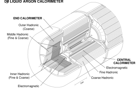
FIG. 1.: A cutaway view of the DØ calorimeter and tracking system.

B Central Detector

The central detector is designed to measure the trajectories of charged particles. It consists of a vertex drift chamber, a transition radiation detector, a central drift chamber (CDC), and two forward drift chambers (FDC). There is no central magnetic field, and DØ therefore cannot distinguish particles by their electric charge, with the exception of muons which penetrate the outer toroidal magnets. Consequently, in the rest of this paper, the term electron will refer to either an electron or a positron. The CDC covers the detector pseudorapidity region $|\eta_{\rm det}|<1.0$. It is a drift chamber with delay lines that give the hit coordinates along the beam direction ($z$) and transverse to the beam ($r$, $\phi$). The FDC covers the region $1.4<|\eta_{\rm det}|<3.0$.

C Calorimeter

The sampling calorimetry is contained in three cryostats, each primarily using uranium absorber plates and liquid argon as the active medium. There is a central calorimeter (CC) and two end calorimeters (EC). Each is segmented into electromagnetic (EM) sections, a fine hadronic (FH) section, and coarse hadronic (CH) sections, with increasingly coarser sampling. The entire calorimeter is divided into about 5000 pseudo-projective towers, each covering 0.1$\times$0.1 in $\eta\times\phi$. The EM section is segmented into four layers which are 2, 2, 7, and 10 radiation lengths in depth respectively. The third layer, in which electromagnetic showers reach their maximum energy deposition, is further segmented into cells covering 0.05$\times$0.05 in $\eta\times\phi$. The hadronic sections are segmented into four (CC) or five (EC) layers. The entire calorimeter is 7–9 nuclear interaction lengths thick. There are no projective cracks in the calorimeter, and it provides hermetic and nearly uniform coverage for particles with $|\eta_{\rm det}|<4$.

D Trigger

Readout of the detector is controlled by a multi-level trigger system. The lowest level hardware trigger consists of two arrays of scintillator hodoscopes, which register hits with a 220 ps time resolution and are mounted in front of the EC cryostats. Particles from the breakup of the proton and the antiproton produce hits in hodoscopes at opposite ends of the CC, each of which are tightly clustered in time. At the lowest trigger level, the detector has a 98.6% acceptance for $W$/$Z$ boson production. For events that contain only a single $p\overline{p}$ interaction, the location of the interaction vertex can be determined from the time difference between the hits at the two ends of the detector to an accuracy of 3 cm. This interaction vertex is used in the last level of the trigger.

The next trigger level consists of an AND-OR decision network programmed to trigger on a $p\overline{p}$ crossing when several preselected conditions are met. This decision is made within the 3.5 $\mu$s time interval between beam bunch crossings. The signals from 2$\times$2 arrays of calorimeter towers (“trigger towers”), covering 0.2$\times$0.2 in $\eta\times\phi$, are added together electronically for the EM sections (“EM trigger towers”) as well as for all sections, and shaped with a fast rise time for use at this trigger level. An additional trigger processor can be invoked to execute simple algorithms on the limited information available at the time of the AND-OR network. These algorithms use the energy deposits in each of the calorimeter trigger towers.

The final software-based level of the trigger consists of an array of 48 VAXstation 4000 computers. At this level, complete event information is available and more sophisticated algorithms are used to refine the trigger decisions. Events are accepted based on certain preprogrammed conditions and are recorded for eventual offline reconstruction.

III Data Selection

A Trigger Filter Requirements

We require the transverse energy, $E_{T}$ ($E\sin\theta$), of one or more trigger towers to be greater than 10 GeV. The trigger processor computes an EM transverse energy by combining the $E_{T}$ of the EM trigger tower (that exceeded some threshold) with the largest signal in the adjacent EM trigger towers, but doing this only if the original EM signal has at least 85% of the energy of the entire trigger tower (including hadronic layers).

For the accepted trigger tower, a software algorithm finds the most energetic of four sub-towers, and sums the energy in a 3$\times$3 array of calorimeter cells around it. It examines the longitudinal shower profile by checking the fraction of the total energy found in different EM layers. The transverse shower shape is characterized by the pattern of energy deposition in the third EM layer. The difference between the energies in concentric regions centered on the most energetic tower covering 0.25$\times$0.25 and 0.15$\times$0.15 in $\eta\times\phi$ must be consistent with expectations for an electron shower. The trigger also imposes an isolation condition requiring

$$\frac{\sum_{i}E_{i}\sin\theta_{i}-p_{T}^{e}}{p_{T}^{e}}<0.15$$ (6)

where the sum runs over all cells within a cone of radius ${\cal R}=\sqrt{\Delta\phi^{2}+\Delta\eta^{2}}=0.4$ around the electron direction and $p_{T}^{e}$ is the transverse momentum of the electron, based on its energy and the $z$-position of the interaction vertex as measured by the hodoscopes.

The trigger requires two electrons which satisfy the isolation requirement, each with $E_{T}$$>$20 GeV. Figure 2 shows the measured detection efficiency of the electron filter as a function of $p_{T}^{e}$ for a threshold of 20 GeV. We determine this efficiency using $Z$ boson data taken with a lower threshold value (16 GeV). (The efficiency corresponds to the fraction of electrons found at the higher threshold.) The curve is a parameterization used in the simulation described in Section III D.

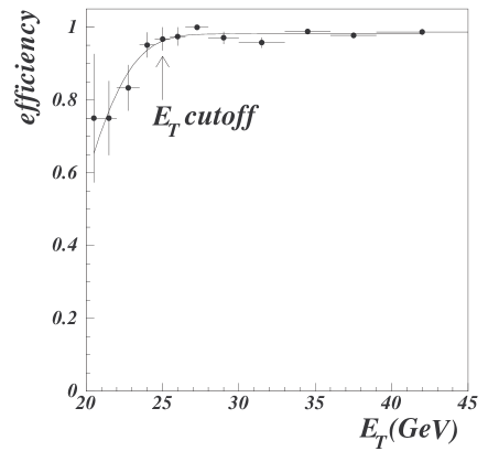
FIG. 2.: Electron detection efficiency as a function of electron $E_{T}$ at the trigger level. The efficiency is essentially flat above our final $E_{T}$ cutoff of $25$ GeV.

B Fiducial and Kinematic Requirements

Events passing the filter requirement are analyzed offline where they are reconstructed with finer precision. The two highest-$E_{T}$ electron candidates in the event, both having $E_{T}$$>$ 25 GeV, are used to reconstruct the $Z$ boson candidate. One electron is required to be in the central region, $|\eta_{\rm det}|<1.1$ (CC), and the second electron may be either in the central or in the forward region, $1.5<|\eta_{\rm det}|<2.5$ (EC). This yields two topologies for the selected events: CCCC, where both electrons are detected in the central region, and CCEC, where one electron is detected in the central region and the other in the forward region. In order to avoid areas of reduced response between neighboring $\phi$ modules of the central calorimeter, the $\phi$ of any electron is required to be at least $0.05\times 2\pi/32$ radians away from the position of a module boundary. Finally, the events are required to have an invariant mass near the known value of the $Z$ boson mass, $75<M_{ee}<105$ GeV.

C Electron Quality Criteria

To be acceptable candidates for $Z$ production, both electrons are required to be isolated and to satisfy offline cluster-shape requirements. Additionally, at least one of the electrons is required to have a spatially matching track associated with the reconstructed calorimeter cluster.

The isolation fraction is defined as

$$f_{\rm iso}={E_{\rm cone}-E_{\rm core}\over E_{\rm core}},$$ (7)

where $E_{\rm cone}$ is the energy in a cone of radius ${\cal R}=0.4$ around the direction of the electron, summed over the entire depth of the calorimeters, and $E_{\rm core}$ is the energy in a cone of ${\cal R}=0.2$, summed over only the EM calorimeter. Both electrons in the data sample are required to have $f_{\rm iso}<0.15$.

We test how well the shape of any cluster agrees with that expected for an electromagnetic shower by computing the quality variable $\chi^{2}_{HM}$ for all cell energies using a 41-dimensional covariance matrix called the H-matrix[25]. The covariance matrix is determined from geant-based simulations [26, 27], which were tuned to agree with test beam measurements. Both electrons in the sample are required to have a tight selection of $\chi^{2}_{HM}<100$.

The quality of the spatial match between a reconstructed track and an electromagnetic cluster is defined by the variable

$$\sigma^{2}=\left({\Delta s\over\delta s}\right)^{2}+\left({\Delta z\over\delta z}\right)^{2},$$ (8)

where $\Delta s$ is the distance between the centroid of the cluster in the third EM layer and the extrapolated trajectory of the track along the azimuthal direction, and $\Delta z$ is the analogous distance in the $z$-direction. For EC electrons, $z$ is replaced by $r$, the radial distance from the center of the detector. The parameters $\delta s=0.25$ cm, $\delta z=2.1$ cm, and $\delta r=1.0$ cm, are the resolutions in $\Delta s$, $\Delta z$, and $\Delta r$, respectively. At least one of the candidate electrons is required to have $\sigma<5$ for candidates with $|\eta_{\rm det}|<1.1$ and $\sigma<10$ for candidates with $1.5<|\eta_{\rm det}|<2.5$.

The total integrated luminosity of the data sample is 111 pb^-1. After applying the selection criteria, 6407 events remain, with 3594 events containing both electrons in the central region and 2813 events containing one electron in the central region and one in the forward region. Figure 3 shows the mass and $p_{T}$ distributions (for $75<M_{ee}<105$ GeV) in the final data sample. There are 157 events with $p_{T}$$>$50 GeV, and the event with the largest $p_{T}$ has $p_{T}=280$ GeV.

FIG. 3.: (a) Mass distribution for all accepted electron pairs, and (b) the $p_{T}$ distribution for those pairs with $75<M_{ee}<105$ GeV.

D Resolutions and Modeling of the Detector

Both the acceptance and the resolution-smeared theory are calculated using a simulation technique originally developed for measuring the mass of the $W$ boson [21] and inclusive cross sections of the $W$ and $Z$ bosons [28], with minor differences arising from small differences in the selection criteria. We briefly summarize the simulation here.

The mass of the $Z$ boson is generated according to an energy-dependent Breit-Wigner lineshape. The $p_{T}$ and rapidity ($y$) are chosen randomly from grids created with the computer program legacy [19] which calculates the $Z$ boson cross section for a given $p_{T}$, $y$, and $Q$. For calculating the grids, we use a fixed value for the mass of the $Z$ boson of 91.184 GeV. We match the low-$p_{T}$ and high-$p_{T}$ regions following the algorithm used in the program resbos [19] to produce a grid of $p_{T}$ and $y$ values, weighted by the production cross section, calculated to NNLO. The primary vertex distribution for the event is modeled as a Gaussian with a width of 27 cm and a mean of $-0.6$ cm, corresponding to the width and offset measured in the data. The positions and energies of the electrons are smeared according to the measured resolutions and corrected for offsets in energy scale caused by the underlying event and recoil particles emitted into the calorimeter towers. Underlying events are modeled using data from random inelastic $p\overline{p}$ collisions with the same luminosity profile as the $Z$ sample.

The electron energy and angular resolutions are tuned to reproduce the observed width of the $Z\rightarrow ee$ mass distribution at the $Z$ resonance. The fractional energy resolution can be parameterized as a function of electron energy as $\Delta E/E={\cal C}\oplus{\cal S}/\sqrt{E_{T}}$. The sampling term, $\cal{S}$, was obtained from measurements made in a calibration beam, and is 0.135 GeV^1/2 for the CC and 0.157 GeV^1/2 for the EC  [29, 30]. The constant term, $\cal{C}$ was determined specifically for our selection criteria. In the CC, the value is ${\cal C}=0.014\pm 0.002$ and in the EC the value is ${\cal C}=0.0^{+0.01}_{-0.00}$. The uncertainty is dominated by the statistics of the $Z\rightarrow ee$ sample. The uncertainty in the polar angle of the electrons is parameterized in terms of the uncertainty in the center-of-gravity of the track used to determine the polar angle. Figure  4 compares electrons from $Z$ boson data with simulated results for distributions in electron $E_{T}$, pseudorapidity, and $\phi$.

In addition to the smearing of the electron energies and positions, certain specific features of the experiment are also modeled in the simulation in order to more closely represent the data. A parameterization of the rise in efficiency of the trigger as a function of electron $E_{T}$ is included, as well as a parameterization of the tracking efficiency as a function of electron pseudorapidity. Both efficiencies have a negligible effect on the shape of the $p_{T}$ distribution. Details of the detector simulation can be found in Refs. [31, 32].

FIG. 4.: Comparison of electron $E_{T}$, $\eta$, and $\phi$, from $Z$ boson data (crosses) to results of the detector simulation (dashed).

IV Efficiency

We determine the efficiency of the event selection criteria as a function of the $p_{T}$ of the $Z$ boson, normalizing the result to the integrated total cross section for $Z$ boson production as measured at DØ ($\sigma_{Z}\cdot B(Z\rightarrow ee)=221$ pb)[28].

Of all the selection criteria, the electron isolation requirement has the largest impact on the observed $p_{T}$ of the $Z$ boson. Nearby jet activity spoils the isolation of an electron, causing it to fail the selection criteria. The effect depends upon the detailed kinematics of the event, in particular, the location of hadronic activity (e.g., associated jet production) and the $p_{T}$ of the vector boson.

Two methods have been used to determine the $p_{T}$-dependence of the electron identification efficiency. In the first method, the effect of jet activity near an electron shower is parameterized in terms of the component of the hadronic recoil energy ($u$) projected onto the vector $p_{T}^{e}$. This is denoted as $u_{||}$ [33]. The relationship between $\vec{p}_{T}^{e}$ and $u_{||}$ is illustrated in Fig. 5. We used a combination of simulated electrons and $W$ boson data to obtain the efficiency for identifying electrons as a function of $u_{||}$. Electron showers were generated using the geant detector-simulation program, and the parameters for the simulated electrons (e.g., $E_{T}$, isolation, $\chi^{2}_{HM}$) agreed well with those observed in $W$ boson data[21]. The agreement suggests that the effect of hadronic activity on the electron is well-modeled in the simulation. Although our parameterization is obtained using electrons from $W$ events, we apply it to electrons from $Z$ boson events (which have very similar energy distributions due to hadronic recoil), because the parameterization reflects the effect of hadronic activity on high-$p_{T}$ electrons, regardless of the origin of that activity.

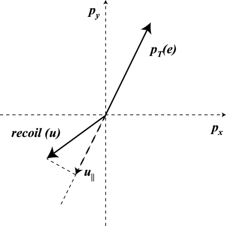
FIG. 5.: Illustration of the relationship between the transverse momentum of the electron, the vector $E_{T}$ of the hadron recoil ($u$) in the calorimeter, and $u_{||}$, the projection of the recoil onto the transverse direction of the electron. In the particular example illustrated here, $u_{||}$ is negative.

The electron identification efficiency as a function of $u_{||}$ is parameterized as:

$$\epsilon(u_{\parallel})=\left\{\begin{array}[]{cc}\alpha&{\rm if}\ (u_{\parallel}<u_{o})\\ \alpha(1-s(u_{\parallel}-u_{o}))&{\rm if}\ (u_{\parallel}>u_{o})\\ \end{array}\right.$$ (9)

where $u_{o}$ is the value of $u_{||}$ at which the efficiency begins to decrease with $u_{||}$, and $s$ is the rate of decrease. The values obtained from the best fit are are $u_{o}=3.85\pm 0.55$ GeV and $s=0.013\pm 0.001$ GeV^-1. The parameter $\alpha$ reflects the overall efficiency, which, as we have indicated, is obtained from a normalization to the overall selection efficiency. The final event efficiency as a function of $p_{T}$ of the $Z$ boson, shown in Fig. 6, is obtained from the detector simulation, by comparing the $p_{T}$ distribution with and without the $u_{||}$ correction. The final event efficiency is insensitive to the use of different parameterizations of the $u_{||}$ efficiency in the EC versus the CC. A more detailed description of the method used to obtain the $u_{||}$ parameterization can be found in Ref. [21].

In the end, the $u_{||}$ parameterization of the event identification efficiency alone is unsatisfactory for application to this measurement. In particular, that analysis required $p_{T}^{W}$$<$30 GeV, thereby restricting applicability to that region. To obtain a reasonable parameterization of the electron identification efficiency for all values of $p_{T}$, we extract the $Z$ boson identification efficiency from events generated with herwig[34], smeared with the DØ detector resolutions, and overlaid onto randomly selected $p\overline{p}$ collisions (“zero-bias” events). The efficiency as a function of $p_{T}$ is defined by the ratio of the $p_{T}$ distribution for events with resolution smearing and kinematic, fiducial and electron quality requirements imposed, to that with only kinematic and fiducial requirements. Figure 6a compares the efficiency as a function of $p_{T}$ using the $u_{||}$ parmeterization with that using the detector-smeared herwig events. The distributions have been normalized to each other in the region $p_{T}$$<$30 GeV. Figure 6(b) shows the ratio of the two normalized results for $p_{T}$$<$30 GeV. The agreement of the herwig analysis with the $u_{||}$ analysis is taken as confirmation of the validity of the herwig result for all $p_{T}$. (The model for the $u_{||}$ analysis has been shown to be reliable for $p_{T}$$<$30 GeV.)

In normalizing our efficiency to the previously determined inclusive $Z$ boson event selection efficiency, we use the combined CCCC and CCEC efficiency of 0.76 [28]. We fit the herwig result to a linear function in the region $p_{T}$$<$18 GeV, and a constant in the region $p_{T}$$>$18 GeV, to obtain the $p_{T}$-dependent event selection efficiency for all $p_{T}$ values. The parameterization is shown in Fig. 7. The $p_{T}$-dependence of the efficiency, in absolute terms, is given by $\epsilon=0.78-0.004p_{T}$, for $p_{T}$$<$ 18 GeV, and 0.73 for $p_{T}$$>$18 GeV.

We assume that the efficiency above 100 GeV is the same as in the region of 18–100 GeV. This is the simplest assumption we can make given the statistics of the simulation. The efficiency at high-$p_{T}$ cannot be greater than at $p_{T}$ = 0, which would correspond to about a 1.5 standard deviation change in the cross section in that region, and this difference would be reflected in the uncertainty on the extracted differential cross section. We do not expect the efficiency to decrease in the region beyond 100 GeV, because the jets in such events will tend to be in the hemisphere opposite to the electrons. Events with high jet multiplicity may have instances in which the large-$E_{T}$ jets balance most of the transverse momentum of the event, but smaller-$E_{T}$ jets can overlap with one of the electrons. However, because the electrons are very energetic, low energy jets are not likely to affect the efficiency of the isolation criteria. We assign estimated uncertainties on the efficiency of $\pm 3$% in the bin below 18 GeV, and $\pm 5$% in the region above 18 GeV.

FIG. 6.: (a) Comparison of the $Z$ boson selection efficiency as a function of $p_{T}$ as determined using herwig (dashed crosses), and as determined using a parameterization of the single-electron efficiency as a function of $u_{||}$ (solid crosses). (b) The ratio of the two methods in the range 0–30 GeV, where they are expected to agree.

FIG. 7.: Final event identification efficiency as a function of $p_{T}$, based on herwig events; the line is the parameterization used in calculating the final cross section.

V Acceptance

The parameterized detector simulation referred to in Section III is used to determine the overall acceptance as a function of $p_{T}$ of the $Z$ boson. The effects of the trigger turn-on in $E_{T}$, the rapidity cut-offs, the $\phi$ module boundaries in the central calorimeter, the pseudorapidity dependence of the tracking efficiency, and the final $E_{T}$ requirements are all included in the calculation of the acceptance. Figure 8 shows the relative effects of the requirements on the electron $E_{T}$ and pseudorapidity, and of the trigger and tracking efficiency on the acceptance as a function of $p_{T}$. As can be seen, the strongest effects come from the electron $E_{T}$ and pseudorapidity requirements. The dip in relative acceptance seen in Fig. 8(a) for middle values of $p_{T}$ results from one of the electrons carrying most of the $p_{T}$ of the $Z$ boson–one electron can have a relatively large $E_{T}$ while the other has relatively small $E_{T}$. However, as the $p_{T}$ of the $Z$ boson increases beyond $45$ GeV, this asymmetry is no longer allowed – both electrons must have relatively large $E_{T}$. The monotonic rise of the relative acceptance in Fig. 8(b) is due to the increasing “centrality” of the event–as $p_{T}$ increases, the rapidity of the $Z$ boson is closer to zero. As can be seen in Figs. 8(c) and (d), the imposition of the other selection criteria merely changes the normalization and does not affect the shape as a function of $p_{T}$.

The mass requirement on the dielectron pairs has been ignored in the final acceptance calculation. Figure 9 compares the $p_{T}$ distribution for dielectron pairs with invariant mass near that of the $Z$ boson to those with invariant mass above and below the nominal $Z$ boson mass, and supports the expectation that any $p_{T}$ dependence on mass (near the $Z$ boson mass peak) is very small.

Figure 10 shows the acceptance for the CCCC and CCEC event topologies, as well as for the combined event sample. Here we see the increased centrality of the events as a function of $p_{T}$, noting the increasing acceptance for the CCCC events in contrast to the decreasing acceptance for the CCEC events. The dip and rise in Fig. 10(b) are due to competing effects of the electron $E_{T}$ and pseudorapidity requirements.

The effect of uncertainties in the energy scale and resolution, the tracking resolution, and the trigger efficiency is assessed for each bin of $p_{T}$ by varying the values of these parameters by their measured uncertainties. Figure 11 shows the nominal acceptance and those obtained by varying the values of the parameters. The largest differences are observed at high $p_{T}$. If we parameterize this systematic uncertainty as a linear function of $p_{T}$, we obtain $\delta_{acc}=\pm(0.01+0.0001p_{T})$. This resulting band of uncertainty is also shown in Fig. 11.

Because we determine the acceptance bin by bin in $p_{T}$, we are relatively insensitive to the underlying model for the $p_{T}$ spectrum used in the detector simulation. Nevertheless, we are sensitive to the assumed rapidity distribution of the $Z$ boson in each bin of $p_{T}$. The uncertainty in the predicted rapidity of the $Z$ boson is expected to be dominated by the uncertainty in the pdf’s used for modeling $Z$ production. The uncertainty in acceptance due to the choice of pdf has been found to be $\pm 0.3\%$ for the inclusive measurement of the $Z$ boson cross section[28]. This constrains the uncertainty in the low-$p_{T}$ region, where the cross section is largest, to a value that is far smaller than the uncertainty from variations in the parameters of the model of the detector. Figure 12 shows that the rapidity distributions obtained from the detector simulation and for data agree for both low and high values of $p_{T}$; we therefore ignore any additional uncertainty in the acceptance due to the modeling of the rapidity of the $Z$ boson.

FIG. 8.: Effect of requirements on (a) $E_{T}$, (b) $\eta$, (c) trigger $E_{T}$ cut-off, and (d) tracking efficiency on the relative acceptance as a function of $p_{T}$.

FIG. 9.: Comparison of the transverse momentum distribution of dielectron pairs with mass very close to the nominal $Z$ boson mass, $90<M_{ee}<92$ GeV (solid circles) to those in the mass regions $75<M_{ee}<90$ GeV (open circles) and $92<M_{ee}<105$ GeV (closed triangles).

FIG. 10.: Final acceptance as a function of $p_{T}$ for (a) the CCCC, (b) CCEC event topologies, and (c) for the combined event sample.

FIG. 11.: Effect of uncertainties on the acceptance in each bin of $p_{T}$. The band corresponds to a parameterization of the uncertainty as a function of $p_{T}$, as discussed in the text.

FIG. 12.: Comparison of $Z$ boson rapidity ($y$) distribution for the data (solid) and the simulation (dashed) for (a) all values of $p_{T}$, (b) $p_{T}$$<$20 GeV, and (c) 20$<$$p_{T}$$<$50 GeV.

VI Backgrounds

The primary background to dielectron production at the Tevatron is from multiple-jet production from QCD processes in which the jets have a large electromagnetic component (most of the energy is deposited in the EM section of the calorimeter) or they are mismeasured in some way that causes them to pass the electron selection criteria. There are also contributions to the $Z$ boson dielectron signal that are not from misidentification of electrons, but correspond to other processes that differ from the one we are trying to measure, e.g., $Z\rightarrow\tau^{+}\tau^{-}$ and $t\overline{t}$ production. Such processes are irreducible due to the fact that they have the same final event signature as the signal, and often have $p_{T}$ dependences that can differ from the $Z$/$\gamma^{*}$ mediated production of the $Z$ boson and Drell-Yan pairs. These must be determined and accounted for in any comparison of data with theory.

Both the normalization and the shape of the multijet background as a function of $p_{T}$ are determined from data. Three types of backgrounds have been studied to examine whether differences in production mechanism or detector resolution would produce a significant variation in the background: dijet events (from multijet triggers), direct-$\gamma$ events (from single photon triggers), and dielectron events in which both electrons failed the quality criteria (from the $Z$ boson trigger). For the dijet events, we selected the two highest-$E_{T}$ jets and reconstructed the “$Z$ boson” as if the jets were electrons. Similarly, for the direct-$\gamma$ events, we selected the highest-$E_{T}$ photon candidate and the highest-$E_{T}$ jet in the event. For the failed-dielectron sample, we used the two highest-$E_{T}$ electron candidates whose cluster shape variable ($\chi_{HM}^{2}$) did not match well with that of an electron. For all three backgrounds, the “electron” objects were required to satisfy the same $E_{T}$ and $\eta$ criteria as the data sample.

Figures 13–16 show the invariant mass and $p_{T}$ distributions for the background samples in both the CCCC and CCEC event topologies. The direct-photon and failed-dielectron events agree in the mass and $p_{T}$ distributions. The Kolmogorov-Smirnov probability ($P_{KS}$) for the two mass distributions is 0.78 and between the two $p_{T}$ distributions it is 0.97. The $p_{T}$ distribution from the dijet sample also agrees well with the direct-$\gamma$ and failed-dielectron samples, with $P_{KS}=0.51$ and $P_{KS}=0.57$, respectively. The dijet mass distribution does not agree as well, giving $P_{KS}=0.005$ when comparing to the direct-$\gamma$ sample and $P_{KS}=0.1$ when comparing to the failed-dielectron sample. The difference is likely due to the poorer jet-energy resolution compared to the electron energy resolution. This difference in the shape of the invariant mass is included in the systematic uncertainty on the background normalization, and is a small effect (see Section VI A).

FIG. 13.: Invariant mass distributions for the three types of QCD multijet background samples in the CCCC topology: (a) dijet data sample, (b) direct-$\gamma$ data sample, (c) failed-dielectron data sample. We show the distributions for all three data samples in (d).

FIG. 14.: Invariant mass distributions for the three types of QCD multijet background samples in the CCEC topology: (a) dijet data sample, (b) direct-$\gamma$ data sample, (c) failed-dielectron data sample. We show the distributions for all three data samples in (d).

FIG. 15.: Comparison of shapes of transverse momentum distributions for the three multijet background samples for the CCCC event topology.

FIG. 16.: Comparison of shapes of transverse momentum distributions for the three multijet background samples for the CCEC event topology.

A Multijet Background Level

Because the mass distribution for the multijet background samples depends on event topology, the level of the multijet background is determined separately for CCCC and CCEC dielectron events. Using this background, and the contribution from the $Z$ boson, we can obtain the relative background fraction through a maximum-likelihood fit for the amount of background and signal in the data.

We use the pythia event generator [35] to produce the invariant mass spectrum for the signal. Contributions from both $Z$ boson and Drell-Yan production and their quantum-mechanical interference are included in the calculation. The generated four-momenta are smeared using the detector simulation described previously. We obtain the amount of multijet background in the data by performing a binned maximum-likelihood fit to the sum of the signal (pythia) and background:

$$N_{\rm data}(m_{i})=c_{1}N_{{\sc pythia}}(m_{i})+c_{2}N_{\rm background}(m_{i})$$ (10)

where $c_{1}$ and $c_{2}$ are the normalization factors for the signal and background contributions, respectively, and $m_{i}$ is the $i$th mass bin. The fit was performed in the dielectron invariant mass window of $60<M_{ee}<120$ GeV. Figure 17 shows the best fit to the dielectron invariant mass, separately for CCCC and CCEC topologies using the direct-$\gamma$ sample as the background. Using the other two background samples yields similar results. The final value for the fraction of multijet background in the data, $f_{\rm back}$, is defined by normalizing the fit parameter $c_{1}$ to the number of events observed in the mass window of the $Z$ boson ($75<M_{ee}<105$ GeV):

$$f_{\rm back}=c_{1}{N_{\rm total}({\rm data})\over N_{\rm total}({\rm background})}{N_{75-105}({\rm background})\over N_{75-105}({\rm data})}$$ (11)

where

$$N_{\rm total}({\rm sample})=\sum_{\rm all\ m_{i}}N_{\rm sample}(m_{i})$$ (12)

$$N_{75-105}({\rm sample})=\sum_{75<m_{i}<105}N_{\rm sample}(m_{i}).$$ (13)

We use the direct-$\gamma$ sample for the central value of the level of multijet background, and use the statistical uncertainty from that fit. We also assign a systematic uncertainty associated with our choice of mass window used in the fit and for differences in the background models. We assign a systematic uncertainty to the background normalization that corresponds to half of the maximum difference from the central value in the determined background fractions. The background values for each topology and the resulting uncertainties are summarized in Table I.

Combining the uncertainties in quadrature, we obtain a background fraction of ($2.45\pm 0.50$)% for the CCCC topology and ($7.09\pm 1.00$)% for the CCEC topology. Weighting the background fractions by the relative number of events in each topology, we obtain a total multijet background level of (4.44$\pm$0.89)%.

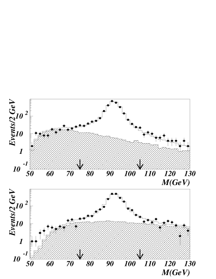
FIG. 17.: Comparison of the dielectron invariant mass distribution (closed circles) and the background (dashed line) to the fit to pythia $Z$/$\gamma^{*}$ and background (solid line) for (a) CCCC and (b) CCEC topologies.

Background Model	CCCC	CCEC
direct-$\gamma$	($2.45\pm 0.41$%)	($7.09\pm 0.87$%)
$55<M_{ee}<125$	($2.10\pm 0.36$%)	($7.52\pm 0.83$%)
$65<M_{ee}<115$	($2.74\pm 0.51$%)	($6.84\pm 0.96$%)
dijets	($1.98\pm 0.35$%)	($6.37\pm 0.80$%)
failed dielectrons	($2.10\pm 0.37$%)	($6.22\pm 0.78$%)
model uncertainty	0.24%	0.44%
window uncertainty	0.17%	0.22%

TABLE I.: Background fractions in the two primary event topologies. The values in the first five rows include only statistical uncertainties for each method. The systematic uncertainties obtained by considering variations in the background selection and fitting criteria are shown in the last two rows.

B $p_{T}$-Dependence of the Multijet Background

The direct-$\gamma$ sample is used to determine the shape of the background distribution for several reasons. First, this sample has the greatest number of events. Second, we expect the direct-$\gamma$ data sample to provide a good approximation of the combination of backgrounds from dijet and true direct-$\gamma$ production because about half of the direct-$\gamma$ sample consists of misidentified dijets, and therefore has the approximate balance of dijet and direct-$\gamma$ events expected from QCD sources. Third, since events in the direct-$\gamma$ often contain at least one good electron-like object, detailed differences between choosing electron-like objects and jet objects for reconstructing the “$Z$” boson are smaller here.

The final shape of the background is obtained by combining the CCCC and CCEC samples, weighted by the relative contributions to the background. To facilitate later analysis, the shape is parameterized as a function of $p_{T}$ using the following functional forms:

$$\begin{array}[]{cc}a(p_{T}+b)^{2}e^{\alpha p_{T}}&{\rm if}\ (p_{T}<8\ {\rm GeV})\\ a({1\over p_{T}})^{2}+be^{\alpha p_{T}}&{\rm if}\ (p_{T}>8\ {\rm GeV})\\ \end{array}$$ (14)

The function is normalized to be a probability distribution, that is the product of the function and the total number of background events results in the differential background in each bin of $p_{T}$. Figure 18 shows the results of the fit to the background and Table II shows the values of the fit parameters.

Parameter	$p_{T}<8$ GeV	$p_{T}>8$ GeV
$\alpha$	$-0.31\pm 0.02$	$-0.1014\pm 0.0015$
$a$	$0.001\pm 0.002$	$0.08\pm 0.03$
$b$	$0.65\pm 0.18$	$0.136\pm 0.004$

TABLE II.: Values of the parameters obtained from the fit to the direct-$\gamma$ background.

C Other Sources of Dielectron Signal

Although $Z\rightarrow ee$ and QCD multijet events make up nearly all of observed dielectron signal, there

FIG. 18.: The results of the fit to the background as a function of $p_{T}$. For (a) $p_{T}$$<$8 GeV, the $\chi^{2}/{\rm d.o.f.}=0.9$, and (b) for $p_{T}$$>$8 GeV, the $\chi^{2}/{\rm d.o.f.}=0.7$.

are contributions from other sources, such as $Z\rightarrow\tau^{+}\tau^{-}$, $t\overline{t}$, and diboson ($WW$, $ZZ$, $WZ$, $W\gamma$, $Z\gamma$) production in dielectron final states. The expected contributions from these sources are estimated below.

The dielectron event rate from $Z\rightarrow\tau^{+}\tau^{-}$ production in our accepted mass range is calculated to be $<2.6\times 10^{-6}$ per $Z\rightarrow ee$ event[36]. The events were generated with the herwig simulator and smeared with the DØ detector resolutions. For the current sample, this corresponds to less than $0.009$ events for all values of dielectron $p_{T}$. We therefore ignore this contribution to the signal.

The dielectron background contribution from $t\overline{t}$ production is concentrated at high $p_{T}$. The fraction was determined using the herwig simulator for $t\overline{t}$ production, smeared with the known DØ detector resolutions. Electron contributions from both $W\rightarrow e\nu$ and $W\rightarrow\tau X\rightarrow eX$ channels were considered. For a $t\overline{t}$ cross section of 6.4 pb[27], and the standard branching ratios for the $W$ boson, the calculated geometric and kinematic acceptance from herwig is $0.01\pm 0.006$. Including electron identification efficiency for dielectron events, we expect about $0.36$ events in the entire sample and about $0.2$ events with dielectron $p_{T}$$>50$ GeV. Considering the small number of events expected, the $t\overline{t}$ contribution is also ignored.

Process	Acceptance	$\sigma\cdot B$ (pb)	Expected events
$t\overline{t}$	0.01$\pm$0.006	0.43$\pm$0.01	$\approx$0.2
$W\gamma$	$<$0.0003	11.3$\pm$0.3	$<.3$
$WW$	0.016$\pm$0.007	0.12$\pm$0.03	$\approx$0.15
$WZ$	0.016$\pm$0.007	0.08$\pm$0.01	$\approx$0.1
$ZZ$	0.046$\pm$0.002	0.03$\pm$0.01	$\approx$0.005

TABLE III.: The expected number of events from diboson and top quark processes. Each channel assumes a total luminosity of 108.5 pb^-1, and a dielectron identification efficiency of 0.73.

We considered $WW$, $ZZ$, $WZ$, and $W\gamma$ events generated with the herwig simulator and smeared with the known DØ detector resolutions. All of these backgrounds are small, and we therefore focus on any possible effects on our measurement at high-$p_{T}$, where there are relatively few events and effects of even a small background contamination could be significant.

The resulting acceptances and expected number of background events with $p_{T}$$>$50 GeV are given in Table III. No $W\gamma$ events out of approximately 3000 generated passed the selection requirements, because very few such events have photons with $E_{T}$$>$25 GeV and an invariant mass ($M_{e\gamma}$) near the $Z$ boson mass. The table includes the assumed production cross sections multiplied by branching ratios ($\sigma\cdot B$) for $W$ and $Z$ boson into electron states. The $WW$ cross section ($10.2^{+6.3}_{-5.1}$ pb) and branching ratio to dielectrons (0.011) are obtained from Ref. [37]. The value $\sigma(W\gamma)\cdot B(W\rightarrow e\nu)=11.3^{+1.7}_{-1.5}$ pb, is obtained from Ref. [38], and assumes $p^{\gamma}_{T}>10$ GeV and $\Delta R_{e\gamma}>0.7$. The standard model $WZ$ cross section is taken from Ref. [39], and the $ZZ$ cross section is taken from Ref. [40]. Given their small size, all of these contributions have been ignored in our analysis.

VII Measured $d\sigma/dp_{T}$

Table IV shows the values for each of the individual components of the measurement: the number of events observed for each bin of $p_{T}$, the product of the efficiency and the acceptance ($\epsilon\cdot a$), and the expected number of background events ($b$). The associated uncertainties are also included. We combine the geometric acceptance and identification efficiencies into a single overall event efficiency by taking their product. We assume that the uncertainties are well-described as Gaussian distributions and add them in quadrature to obtain the uncertainty $\delta(\epsilon\cdot a)$.

The measured differential cross section, $d\sigma^{\prime}/dp_{T}$, is obtained by calculating the cross section in each bin of $p_{T}$, accounting for the effects of efficiency, acceptance, and background, but not accounting for the effects of detector smearing. That is,

$$({d\sigma^{\prime}\over dp_{T}})_{i}={\sigma^{\prime}_{i}\over\Delta_{i}^{\text{b}in}}.$$ (15)

where $\sigma^{\prime}_{i}$ is the measured cross section in bin $i$ and $\Delta_{i}^{\text{b}in}$ is the width of the bin in $p_{T}$.

We obtain the cross section and uncertainty in each bin using the methods of statistical inference. We relate the expected number of events $\mu$ in each bin to the underlying cross section [41, 42]:

$$\mu={\cal{L}}\epsilon\sigma^{\prime}+b,$$ (16)

where $\cal{L}$ is the total integrated luminosity, $\epsilon$ is the overall detection efficiency for the process, and $b$ is the number of background events. A value of $\mu$ is determined for each bin of $p_{T}$.

We relate the observed number of events and the expected number of events through a probability distribution, in our case an assumed Poisson distribution,

$$P(d|\sigma^{\prime},\epsilon,b,{\cal{L}},I)={e^{-({\cal{L}}\epsilon\sigma^{\prime}+b)}({\cal{L}}\epsilon\sigma^{\prime}+b)^{d}\over d!}.$$ (17)

where $d$ is the number of events observed and $I$ refers to the assumptions implicit in deriving the probability density[42].

Applying Bayes’ Theorem, we invert the probability in Eq. 17,

$$P(\sigma^{\prime},\epsilon,b,{\cal{L}}|d,I)=\\ {P(d|\sigma^{\prime},\epsilon,b,{\cal{L}},I)P(\sigma^{\prime},\epsilon,b,{\cal{L}}|I)\over\zeta}$$ (18)

where $\zeta$ normalizes the probability such that $\int P(\sigma^{\prime},\epsilon,b,{\cal{L}}|d,I)d\Omega\equiv 1$, where $d\Omega$ denotes that the integration is over all relevant variables. $P(\sigma^{\prime},\epsilon,b,{\cal{L}}|d,I)$ is the joint posterior probability, describing the probability of a particular set of $\sigma^{\prime},\epsilon,b$, and $\cal{L}$  given the results from our data. $P(\sigma^{\prime},\epsilon,b,{\cal{L}}|I)$ is the joint prior probability, describing the probability of a particular set of $\sigma^{\prime},\epsilon,b$, $\cal{L}$ before taking our data into account. $P(d|\sigma^{\prime},\epsilon,b,{\cal{L}},I)$ is the likelihood function for our data. Assuming that the individual parameters are logically independent, e.g., the cross section does not depend on the background, then Eq. 18 can be rewritten as

$$P(\sigma^{\prime},\epsilon,b,{\cal{L}}|d,I)=\\ {P(d|\sigma^{\prime},\epsilon,b,{\cal{L}},I)P(\sigma^{\prime}|I)P(\epsilon|I)P(b|I)P({\cal{L}}|I)\over\zeta}.$$ (19)

We are not interested in the values of the parameters $\epsilon$, $b$, and $\cal{L}$, and we eliminate the dependence of the joint posterior probability on these nuisance parameters by integrating over their allowed values,

FIG. 19.: The measured differential cross section, not corrected for detector smearing, (a) for $p_{T}$$<$50 GeV and (b) for all $p_{T}$.

a process called marginalization. To extract our results, we calculate

$$P(\sigma^{\prime}|d,I)=\int dbd{\cal{L}}d\epsilon d\sigma^{\prime}\\ {P(d|\sigma^{\prime},\epsilon,b,{\cal{L}},I)P(\sigma^{\prime}|I)P(\epsilon|I)P(b|I)P({\cal{L}}|I)\over\zeta}.$$ (20)

In the calculation of the binned differential cross section, the uncertainty on the integrated luminosity changes only the overall normalization of the distribution, which is already accounted for in our normalization to the DØ measurement of $\sigma_{Z\rightarrow ee}$. We therefore use a delta function as the prior for the integrated luminosity distribution. We assume the priors for the efficiency ($\epsilon$) and background ($b$) to be Gaussian distributed, with their estimated mean values and standard deviations as the means and widths of the Gaussians. The prior probability distribution for the cross section in each bin is taken to be independent of $\sigma$ (uniform for the range $[\sigma_{min},\sigma_{max}]$ where $\sigma_{min}>0$) and the total range is at least $\pm$6 standard deviations around the mean.

The integration in Eq. 20 is performed using the numerical integrator miser [43], and the results are shown in Fig. 20. Since the probability distributions for all but the highest-$p_{T}$ bin are nearly Gaussian, we assign the final value of the cross section for each bin in $p_{T}$ to be the mean of the probability distribution with uncertainties set equal to the standard deviation about the mean. For the highest-$p_{T}$ bin, we use the most probable value for the cross section with upper and lower uncertainty values circumscribing the narrowest 68% confidence interval. The integral over $p_{T}$ of the differential distribution is normalized to the inclusive cross section for $Z$ boson production measured by DØ [28]. Table IV gives the values of the measured differential cross section in each bin of $p_{T}$, not corrected for detector smearing, and Figure 19 displays the results as a function of $p_{T}$.

VIII Fit to Non-perturbative Parameters

As discussed in Section I, the current theoretical understanding of the $p_{T}$ distribution of $Z$ bosons uses fixed-order perturbative calcuations to describe the high-$p_{T}$ region and resummation calculations of the perturbative solution to describe the low-$p_{T}$ region. At the smallest values of $p_{T}$, a parameterization must be invoked to account for non-perturbative effects that are not calculable in perturbative QCD. The generic form for the function is given in Eq. 4, however, one must choose particular functional forms for $h_{1}(x,b)$ and $h_{2}(b)$. Historically there are two versions for the choice of this parameterization. The first, from Davies, Weber, and Stirling (DWS)[15], has the form:

$$S_{NP}^{DWS}(b,Q^{2})=g_{1}b^{2}+g_{2}b^{2}\ln({Q^{2}\over Q_{o}^{2}}).$$ (21)

The values of $g_{1}$ and $g_{2}$ are determined by fitting to low-energy Drell-Yan data, yielding $g_{1}=0.15$ GeV² and $g_{2}=0.4$ GeV², where $Q_{o}=2$ GeV and $b_{max}=0.5$ GeV^-1 (see Eq. 3). They used the pdf’s of Duke and Owens [45]. The second is from Ladinsky and Yuan[18]:

$$S_{NP}^{LY}(b,Q^{2})=$$ (22)

$$g_{1}b^{2}+g_{2}b^{2}\ln({Q^{2}\over Q_{o}^{2}})+g_{1}g_{3}b\ln(100x_{i}x_{j})$$ (23)

where $x_{i}$ and $x_{j}$ are the momentum fractions of the colliding partons. The values of $g_{1}$, $g_{2}$, and $g_{3}$ are determined by fitting to low-energy Drell-Yan data and a small sample of $Z\rightarrow ee$ data from the 1988–89 run at CDF[12], yielding $g_{1}=0.11^{+0.04}_{-0.03}$ GeV², $g_{2}=0.58_{-0.2}^{+0.1}$ GeV², and $g_{3}=-1.5_{-0.1}^{+0.1}$ GeV^-1, where $b_{max}=0.5$ GeV^-1 and $Q_{o}=1.6$ GeV. They used the CTEQ2M pdf’s [46] in the fits.

The $Z$ boson $p_{T}$ distribution is by far most sensitive to the value of $g_{2}$. For measurements at the Tevatron at $Q^{2}=M_{Z}^{2}$, the calculation is nearly insensitive to the value of $g_{3}$, and only slightly sensitive to the value of $g_{1}$. For $g_{3}$, this insensitivity is due to the high energy of the $p\overline{p}$ beam relative to the $Q^{2}$ being probed. For a center-of-mass energy of $\hat{s}=x_{i}x_{j}s$ and $\hat{s}\approx M_{Z}^{2}$, we see that for a measurement at the Tevatron ($\sqrt{s}=1.8$ TeV), the $g_{3}$ term becomes $g_{1}g_{3}b\ln(100\hat{s}/s)\approx-1.4g_{1}g_{3}b$. The $g_{2}$ term varies as $g_{2}b^{2}\ln(M_{Z}/Q_{o})\approx 4.7g_{2}b^{2}$, and therefore makes a far larger contribution to the value of $S_{NP}$. The relative importance of $g_{2}$ over $g_{1}$ comes from the $\ln({Q^{2}/Q_{o}^{2}})$ term.

Because the width of the $Z$ boson is $\approx 2.5$ GeV, for purely phenomenological needs the non-perturbative physics can be parameterized using a single parameter $g^{\prime}=g_{1}+g_{2}\log({M_{Z}^{2}/Q_{o}^{2}})$ [44]. However, because the general form of $S_{NP}$ is theoretically motivated, we preserve the form of Eq. 22, focusing on the value of $g_{2}$, the parameter we are most sensitive to.

We perform a minimum-$\chi^{2}$ fit to determine the best value of $g_{2}$ from our data. For the purposes of the fit, we fix $g_{1}=0.11$ GeV² and $g_{3}=-1.5$ GeV^-1, as suggested by Ladinsky and Yuan [18]. We use the program legacy [19] with the CTEQ4M pdf’s [47] to generate the $d\sigma^{\prime}/dp_{T}$ distribution for the $Z$ boson and match the low-$p_{T}$ and high-$p_{T}$ regions using the prescription in resbos, obtaining a single grid for all values of $p_{T}$ calculated to NNLO. We smear the prediction with the DØ detector resolutions and fit the resulting $p_{T}$ distribution to our measured result. The $\chi^{2}$ distribution as a function of $g_{2}$ is well-behaved and parabolic and when fit to a quadratic function yields a value of 0.59$\pm$0.06 GeV² at the minimum, with $\chi^{2}$/d.o.f$=10.6/10$.

For completeness, we also fit for the individual values of $g_{1}$ and $g_{3}$, using the Ladinsky and Yuan values for the two parameters not being fitted. The variation in $\chi^{2}$ of $g_{1}$ and $g_{3}$ are also well-behaved and parabolic, and the fit yields $g_{1}=0.09\pm 0.03$ GeV² and $g_{3}=-1.1\pm 0.6$ GeV^-1. The value of $g_{1}$ agrees with the Ladinsky-Yuan result, and is of comparable precision. The value of $g_{3}$ also agrees with the Ladinsky-Yuan result, but is far less precise.

Bin	$p_{T}$ range	number			$b$	$\delta b$	${d\sigma^{\prime}/dp_{T}}$	$\delta({d\sigma^{\prime}/dp_{T}})$		${d\sigma/dp_{T}}$	$\delta({d\sigma/dp_{T}})$
number	(GeV)	of events	$\epsilon\cdot a$	$\delta(\epsilon\cdot a)$	(events)	(events)	(nb/GeV)	(nb/GeV)	$\alpha(p_{T})$	(nb/GeV)	(nb/GeV)
1	0–1	156	0.351	0.011	3.28	0.7	5.10	0.45	1.185	6.04	0.53
2	1–2	424	0.347	0.011	8.14	1.6	14.0	0.82	1.160	16.2	0.96
3	2–3	559	0.346	0.011	12.7	2.5	18.4	0.99	1.108	20.4	1.1
4	3–4	572	0.343	0.011	16.1	3.2	18.9	1.0	1.042	19.7	1.1
5	4–5	501	0.343	0.011	18.0	3.6	16.4	0.93	0.988	16.2	0.92
6	5–6	473	0.342	0.011	18.8	3.8	15.5	0.90	0.965	15.0	0.87
7	6–7	440	0.336	0.011	18.5	3.7	14.6	0.88	0.960	14.1	0.84
8	7–8	346	0.335	0.011	17.5	3.5	11.5	0.76	0.967	11.1	0.73
9	8–9	312	0.334	0.011	16.9	3.4	10.3	0.71	0.972	10.0	0.69
10	9–10	285	0.330	0.011	15.2	3.1	9.55	0.69	0.972	9.29	0.67
11	10–12	439	0.324	0.017	26.1	5.2	7.46	0.56	0.972	7.25	0.54
12	12–14	326	0.317	0.017	21.3	4.3	5.63	0.46	0.967	5.45	0.44
13	14–16	258	0.306	0.017	17.4	3.5	4.61	0.41	0.964	4.45	0.39
14	16–18	203	0.302	0.016	14.2	2.8	3.67	0.34	0.963	3.54	0.33
15	18–20	181	0.297	0.016	11.6	2.3	3.35	0.32	0.958	3.21	0.31
16	20–25	287	0.289	0.016	20.5	4.1	2.16	0.19	0.954	2.06	0.18
17	25–30	174	0.278	0.015	12.3	2.5	1.37	0.14	0.945	1.29	0.13
18	30–35	124	0.270	0.016	7.46	1.5	1.02	0.12	0.944	0.962	0.11
19	35–40	104	0.263	0.014	4.51	0.90	0.892	0.10	0.941	0.840	0.10
20	40–50	92	0.264	0.014	4.38	0.88	0.392	0.048	0.952	0.373	0.045
21	50–60	61	0.274	0.015	1.63	0.33	0.258	0.037	0.974	0.251	0.036
22	60–70	40	0.283	0.016	0.616	0.12	0.167	0.028	0.975	0.163	0.027
23	70–85	20	0.300	0.017	0.308	0.062	0.054	0.016	0.989	0.053	0.012
24	85–100	13	0.319	0.018	0.095	0.019	0.034	0.010	0.988	0.034	0.009
25	100–200	15	0.366	0.022	0.130	0.026	0.0051	0.0013	0.994	0.0050	0.0013
26	200–300	2	0.530	0.034	0.038	0.0076	0.0004	${}^{+0.00038}_{-0.00029}$	0.994	0.0004	${}^{+0.00038}_{-0.00029}$

TABLE IV.: Summary of the results of the measurement of the $p_{T}$ distribution of the $Z$ boson. The range of $p_{T}$ corresponds to the intervals used for binning the data. The product of the acceptance and efficiency is given as $\epsilon\cdot a$, $b$ is the estimated number of background events, the measured differential cross section is ${d\sigma^{\prime}/dp_{T}}$, the correction for resolution-smearing is specified by $\alpha(p_{T})$, and the corrected differential cross section is specified by ${d\sigma/dp_{T}}$. The uncertainty on the differential cross section includes both systematic and statistical uncertatinties, but does not include overall normalization uncertainty due to the luminosity of $\pm 4.4$%.

FIG. 20.: Normalized probability distributions for cross sections ($\sigma$) in individual bins of $p_{T}$. The vertical scale in each case is Probability/pb.

FIG. 21.: Smearing correction factor $\alpha(p_{T})$ as a function of $p_{T}$.

IX Smearing Corrections

The results shown in Fig. 19 still contain the residual effects of detector smearing. We correct the measured cross section for the effects of detector smearing using the ratio of generated to resolution-smeared ansatz $p_{T}$ distributions:

$$\alpha(p_{T})={F(p_{T};g_{2})\over\int dp_{T}\ R(p_{T},p^{\prime}_{T})F(p_{T};g_{2})}$$ (24)

where $p^{\prime}_{T}$ is the smeared value of $p_{T}$, $\alpha(p_{T})$ is the correction factor, $F(p_{T};g_{2})$ is the ansatz function with parameter $g_{2}$ and $R(p_{T},p^{\prime}_{T})$ is the resolution function.

As the ansatz function, we use the calculation from legacy fixing $g_{1}=0.11$ GeV² and $g_{3}=-1.5$ GeV^-1. We use $g_{2}=0.59$ GeV² for our central value.

Figure 21 shows the smearing correction as a function of $p_{T}$. The largest effect occurs at low-$p_{T}$ where the smearing causes the largest fractional change in $p_{T}$ and where the kinematic boundary at $p_{T}$$=0$ results in non-Gaussian smearing—the $p_{T}$ is preferentially increased by the smearing rather than being a symmetric effect. Table IV includes the value of the smearing correction for each bin of $p_{T}$.

FIG. 22.: Fractional uncertainty in the cross section as a function of $p_{T}$ including the statistical and systematic uncertainties (closed circles) and including only statistical uncertainties (open circles) for (a) $p_{T}<50$ GeV and (b) $p_{T}>50$ GeV.

It is important that the smearing correction be insensitive to significant variations in the ansatz function used to generate the correction. We examine this issue by varying the parameter $g_{2}=0.59\pm 0.06$GeV² in the ansatz function by $\pm 1\sigma$, obtaining a variation of $<$1% for all values of $p_{T}$. For this variation in the parameter, the ansatz function varies by $\approx$10%. It is useful to compare the level of uncertainty in the smearing correction to other components of uncertainty in the measurement. Figure 22 shows the fractional uncertainty on the differential cross section as a function of $p_{T}$. Both the total uncertainties (in which systematic uncertainties on the background, efficiency, and acceptance are included with the statistical uncertainty), and the statistical uncertainties alone are shown. The variations in the smearing correction are at least a factor of five smaller than the other uncertainties and therefore can be ignored.

The uncertainty in the smearing correction is also affected by the uncertainty on the values of the resolutions used to generate the smearing. We examine this uncertainty by varying the detector resolutions by $\pm 1$ standard deviation from the nominal values. Again, the effect on the smearing correction is negligible relative to the other uncertainties in the measurement and this source of uncertainty has been ignored.

FIG. 23.: Plot of the differential cross section (circles) as a function of $p_{T}$. The line is the result of the NNLO calculation from resbos using the CTEQ4M pdf. Theory has been normalized to the data.

X Results

Table IV shows the final numerical results for the measurement of $d\sigma/dp_{T}$ using a total of 6407 events. The uncertainties on the data points include statistical and systematic contributions. There is an additional normalization uncertainty of $\pm$4.4% from the uncertainty on the integrated luminosity [28] that is included in neither the plots nor the table, but must be taken into account in any fits requiring an absolute cross section.

Figures 23–25 and 27 show the final, smearing-corrected $p_{T}$ distribution compared to the fully resummed calculation as calculated by resbos. The calculation uses the CTEQ4M pdf’s and the Ladinsky-Yuan parameterization for the non-perturbative function with the published values for the $g_{i}$ parameters: $g_{1}=0.11$ GeV², $g_{2}=0.58$ GeV², and $g_{3}=-1.5$ GeV^-1. The data points in Figs. 23 and 25 are placed at the average $p_{T}$ of the bin, as given by theory, rather than at the center of the bin. (Only the first and twenty-fifth bins change appreciably, $-24$% and $-17$% respectively, relative to the bin center.) For the resummed calculation, the total cross section predicted by the theory (220 pb) has been normalized to the data. A $\chi^{2}$ comparison of the prediction to the data yields a $\chi^{2}/$d.o.f.$=26.7/25$. We observe good agreement with the fully resummed calculation for all values of $p_{T}$.

FIG. 24.: Fractional difference between the data and the NNLO calculation from resbos for the differential cross section as a function of $p_{T}$.

Figures 26 and 28 compare the data to the fixed-order (NLO) perturbative calculation as calculated by resbos and using the CTEQ4M pdf’s. We observe strong disagreement at low-$p_{T}$, as expected due to the divergence of the NLO calculation at $p_{T}$$=0$, and a significant enhancement of the cross section relative to the prediction at moderate values of $p_{T}$, confirming the increase in the cross section from soft gluon emission.

XI Conclusions

We have measured the differential cross section as a function of the transverse momentum of the $Z$ boson. Fitting for the value of the non-perturbative parameter $g_{2}$, we obtain $g_{2}=0.59\pm 0.06$ GeV², which is significantly more precise than previous determinations. We observe good agreement between the measurement and the resummation calculations for all values of $p_{T}$.

REFERENCES

- [1] UA1 Collaboration, G. Arnison et al., Phys. Lett. B 126, 398 (1983).
- [2] UA2 Collaboration, P. Bagnaia et al., Phys. Lett. B 129, 130 (1983).
- [3] UA1 Collaboration, G. Arnison et al., Phys. Lett. B 122, 103 (1983).
- [4] UA2 Collaboration, P. Bagnaia et al., Phys. Lett. B 122, 476 (1983).
- [5] The LEP Collaborations, the LEP Electroweak Working Group, and the SLD Heavy Flavour Group, Report No. CERN-PPE/97-154 (unpublished).
- [6] Particle Data Group, R.M. Barnett, et al., Phys. Rev. D 54, 1 (1996).
- [7] D. Casey, Ph.D. thesis, University of Rochester, 1997 (unpublished), http://www-d0.fnal.gov/ publications_talks/thesis/casey/thesis.ps.
- [8] J.C. Collins, D.E. Soper, Nucl. Phys. B193, 381 (1981); B213, 545E (1983); J.C. Collins, D.E. Soper, G. Sterman, ibid. B250, 199 (1985).
- [9] S.D. Drell and T.M. Yan, Phys. Rev. Lett. 25, 316 (1970).
- [10] A.S. Ito et al., Phys. Rev. D 23, 604 (1981); D. Antreasyan et al., Phys. Rev. Lett. 47, 12 (1981); 48, 302 (1982).
- [11] CDF Collaboration, F. Abe et al., Phys. Rev. Lett. 66, 2951 (1991); DØ Collaboration, B. Abbott et al., Phys. Rev. Lett. 80, 5498 (1998).
- [12] CDF Collaboration, F. Abe et al., Phys. Rev. Lett. 67, 2937 (1991).
- [13] C.T.H. Davies and W.J. Stirling, Nucl. Phys. B244, 337 (1984).
- [14] G. Altarelli, R.K. Ellis, M. Greco, and G. Martinelli, Nucl. Phys. B246, 12 (1984).
- [15] C.T.H Davies, B.R. Weber, W.J. Stirling, Nucl. Phys. B256, 413 (1985).
- [16] P.B. Arnold and M.H. Reno, Nucl. Phys. B319, 37 (1989); B330, 284E (1990).
- [17] P.B. Arnold and R.P. Kaufman, Nucl. Phys. B349, 381 (1991).
- [18] G.A. Ladinsky and C.-P. Yuan, Phys. Rev. D 50, 4239 (1994).
- [19] C. Balazs and C.-P. Yuan, Phys. Rev. D 56, 5558 (1997).
- [20] G. P. Korchemsky and G. Sterman, Nucl. Phys. B437, 415 (1995).
- [21] DØ Collaboration, B. Abbott et al., Phys. Rev. D 58, 092003 (1998).
- [22] CDF Collaboration, F. Abe et al., Phys. Rev. Lett. 75, 11 (1995).
- [23] UA2 Collaboration, P. Bagnaia et al., Z. Phys. C, 47 523 (1990).
- [24] DØ Collaboration, S. Abachi et al., Nucl. Instr. and Methods in Phys. Res. A 338, 185 (1994).
- [25] DØ Collaboration, S. Abachi et al., Phys. Rev. D 52, 4877 (1995).
- [26] F. Carminati et al., geant Users Guide, CERN Program Library W5013, 1991 (unpublished).
- [27] DØ Collaboration, S. Abachi et al., Phys. Rev. Lett. 74, 2632 (1995); DØ Collaboration, Phys. Rev. D 58, 052001 (1998).
- [28] DØ Collaboration, B. Abbott et al., Fermilab-Pub-00/171-E, hep-ex-9906025, submitted to Phys. Rev. D.
- [29] Q. Zhu, Ph.D. thesis, New York University, 1994 (unpublished), http://www-d0.fnal.gov/public ations_talks/thesis/zhu/thesis_1side.ps.
- [30] T.C. Heuring, Ph.D. thesis, State University of New York at Stony Brook, 1993 (unpublished), http://www-d0.fnal.gov/publications_talks /thesis/heuring/thesis2s.ps.
- [31] I. Adam Ph.D. thesis, Columbia University, 1997 (unpublished), http://www-d0.fnal.gov/public ations_talks/thesis/adam/ian_thesis_all.ps.
- [32] E. Flattum, Ph.D. thesis, Michigan State University, 1997 (unpublished), http://www-d0.fnal. gov/publications_talks/thesis/flattum/eric _thesis.ps.
- [33] CDF Collaboration, F. Abe et al., Phys. Rev. Lett. 65, 2243 (1990).
- [34] G. Marchesini et al., Comput. Phys. Commun. 67, 465 (1992).
- [35] H.U. Bengtsson and T. Sjostrand, Comput. Phys. Commun. 46, 43 (1987).
- [36] Z.Jiang, Ph.D. thesis, State University of New York at Stony Brook, 1995 (unpublished).
- [37] CDF Collaboration, F. Abe et al., Phys. Rev. Lett. 78, 4536 (1997).
- [38] DØ Collaboration, S. Abachi et al., Phy. Rev. Lett. 78, 3634 (1997).
- [39] K. Hagiwara, J. Woodside, and D. Zeppenfeld, Phys. Rev. D 41, 2113 (1990).
- [40] E. Eitchen, I. Hinchliffe, K. Lane, and C. Quigg, Rev. Mod. Phys. 56, 579 (1984).
- [41] T. J. Loredo, “From LaPlace to Supernova SN1987A: Bayesian Inference in Astrophysics,” in Maximum Entropy and Bayesian Methods, edited by P. Fougere (Kluwer Academic Publishers, Dordrecht, the Netherlands) 1990.
- [42] E.T. Jaynes, Probability Theory The Logic of Science, in preparation. Copies of the manuscript are available from http://bayes.wustl.edu.
- [43] W.H. Press et al., Numerical Recipes in C, (Cambridge University Press, London) 1996.
- [44] R.K. Ellis, S. Veseli, Nucl. Phys. B511, 649 (1998).
- [45] D. Duke and J.F. Owens, Phy. Rev. D 30, 49 (1984).
- [46] J. Botts et al., Michigan State University preprint MSUTH-93/17.
- [47] CTEQ Collaboration, H.L. Lai et al., Phys. Rev. D 55, 1280 (1997).