A Measurement of the $W$ Boson Mass

Abstract

We report a measurement of the $W$ boson mass based on an integrated luminosity of 82 pb^-1 from $p\overline{p}$ collisions at $\sqrt{s}=1.8$ TeV recorded in 1994–1995 by the DØ detector at the Fermilab Tevatron. We identify $W$ bosons by their decays to $e\nu$ and extract the mass by fitting the transverse mass spectrum from 28,323 $W$ boson candidates. A sample of 3,563 dielectron events, mostly due to $Z\to ee$ decays, constrains models of $W$ boson production and the detector. We measure $M_{W}=80.44\pm 0.10(\hbox{stat})\pm 0.07(\hbox{syst})$ GeV. By combining this measurement with our result from the 1992–1993 data set, we obtain $M_{W}=80.43\pm 0.11$ GeV.

In the standard model of the electroweak interactions (SM) [3], the mass of the $W$ boson is predicted to be

$$M_{W}=\left(\frac{\pi\alpha(M_{Z}^{2})}{\sqrt{2}G_{F}}\right)^{\frac{1}{2}}\frac{1}{\sin\theta_{w}\sqrt{1-\Delta r}}\;.$$ (1)

In the “on-shell” scheme [4] $\cos\theta_{w}=M_{W}/M_{Z}$, where $M_{Z}$ is the $Z$ boson mass. A measurement of $M_{W}$, together with $M_{Z}$, the Fermi constant ($G_{F}$), and the electromagnetic coupling constant ($\alpha$), determines the electroweak radiative corrections $\Delta r$ experimentally. Purely electromagnetic corrections are absorbed into the value of $\alpha$ by evaluating it at $Q^{2}=M_{Z}^{2}$. The dominant contributions to $\Delta r$ arise from loop diagrams that involve the top quark and the Higgs boson. If additional particles which couple to the $W$ boson exist, they will give rise to additional contributions to $\Delta r$. Therefore, a measurement of $M_{W}$ is one of the most stringent experimental tests of SM predictions. Deviations from the predictions may indicate the existence of new physics. Within the SM, measurements of $M_{W}$ and the mass of the top quark constrain the mass of the Higgs boson.

This Letter reports a precise new measurement of the $W$ boson mass based on an integrated luminosity of 82 pb^-1 from $p\overline{p}$ collisions at $\sqrt{s}=1.8$ TeV, recorded by the DØ detector [5] during the 1994–1995 run of the Fermilab Tevatron. A more complete account of this analysis can be found in Refs. [6, 7, 8]. Previously published measurements [9, 10, 11, 12, 13, 14, 15], when combined, determine the $W$ boson mass to a precision of 125 MeV.

At the Tevatron, $W$ bosons are produced mainly through $q\overline{q}$ annihilation. We detect them by their decays into electron-neutrino pairs, characterized by an isolated electron [16] with large transverse momentum ($p_{T}$) and significant transverse momentum imbalance ($\hbox to0.0pt{\kern 1.00006pt/\hss}p_{T}$). The $\hbox to0.0pt{\kern 1.00006pt/\hss}p_{T}$ is due to the neutrino which escapes detection. Many other particles of lower momenta, which recoil against the $W$ boson, are produced in the breakup of the proton and antiproton. We refer to them collectively as the underlying event.

At the trigger level we require $\mbox{$\hbox to0.0pt{\kern 1.00006pt/\hss}p_{T}$}>15$ GeV and an energy cluster in the electromagnetic (EM) calorimeter with $p_{T}>20$ GeV. The cluster must be isolated and have a shape consistent with that of an electron shower.

During event reconstruction, electrons are identified as energy clusters in the EM calorimeter which satisfy isolation and shower shape cuts and have a drift chamber track pointing towards the cluster centroid. We determine their energies by adding the energy depositions in the first $\approx 40$ radiation lengths of the calorimeter in a window, spanning 0.5 in azimuth ($\phi$) by 0.5 in pseudorapidity ($\eta$) [17], centered on the highest energy deposit in the cluster. Fiducial cuts reject electron candidates near calorimeter module edges and ensure a uniform calorimeter response for the selected electrons. The electron momentum ($\vec{p}(e)$) is determined by combining its energy with its direction which is obtained from the shower centroid position and the drift chamber track. The trajectories of the electron and the proton beam define the position of the event vertex.

We measure the sum of the transverse momenta of all the particles recoiling against the $W$ boson, $\vec{u}_{T}=\sum_{i}E_{i}\sin\theta_{i}\hat{u}_{i}$, where $E_{i}$ is the energy deposition in the $i^{th}$ calorimeter cell and $\theta_{i}$ is the angle defined by the cell center, the event vertex, and the proton beam. The unit vector $\hat{u}_{i}$ points perpendicularly from the beam to the cell center. The calculation of $\vec{u}_{T}$ excludes the cells occupied by the electron. The sum of the momentum components along the beam is not well measured because of particles escaping through the beam pipe. From momentum conservation we infer the transverse neutrino momentum, $\vec{p}_{T}(\nu)=-\vec{p}_{T}(e)-\vec{u}_{T}$, and the transverse momentum of the $W$ boson, $\vec{p}_{T}(W)=-\vec{u}_{T}$.

We select a $W$ boson sample of 28,323 events by requiring $p_{T}(\nu)>25$ GeV, $u_{T}<15$ GeV, and an electron candidate with $|\eta|<1.0$ and $p_{T}(e)>25$ GeV.

Since we do not measure the longitudinal momentum components of the neutrinos from $W$ boson decays, we cannot reconstruct the $e\nu$ invariant mass. Instead, we extract the $W$ boson mass from the spectra of the electron $p_{T}$ and the transverse mass, $m_{T}=\sqrt{2p_{T}(e)p_{T}(\nu)(1-\cos\Delta\phi)}$, where $\Delta\phi$ is the azimuthal separation between the two leptons. We perform a maximum likelihood fit to the data using probability density functions from a Monte Carlo program. Since neither $m_{T}$ nor $p_{T}(e)$ are Lorentz invariants, we have to model the production dynamics of $W$ bosons to correctly predict the spectra. The $m_{T}$ spectrum is insensitive to transverse boosts at leading order in $p_{T}(W)/M_{W}$ and is therefore less sensitive to the $W$ boson production model than the $p_{T}(e)$ spectrum. On the other hand, the $m_{T}$ spectrum depends strongly on the detector response to the underlying event and is therefore more sensitive to detector effects than the $p_{T}(e)$ spectrum.

$Z$ bosons decaying to electrons provide an important control sample. We use them to calibrate the detector response to the underlying event and to the electrons, and to constrain the model for intermediate vector boson production used in the Monte Carlo simulations.

A $Z\to ee$ event is characterized by two isolated high-$p_{T}$ electrons. We trigger on events with at least two EM clusters with $p_{T}>20$ GeV. We define two samples of $Z\to ee$ decays in this analysis. For both $Z$ samples, we require two electron candidates with $p_{T}>25$ GeV. For sample I, we loosen the pseudorapidity cut for one of the electrons to $|\eta|<2.5$. This selection accepts 2,341 events. For sample II, we require both electrons with $|\eta|<1.0$ but allow one electron without a matching drift chamber track. Relaxing the track requirement for electrons with $|\eta|<1.0$ increases the efficiency without a significant increase in background. Sample II contains 2,179 events of which 1,225 are in common with sample I.

For this measurement we developed a fast Monte Carlo program that generates $W$ and $Z$ bosons with the rapidity and $p_{T}$ spectra given by a calculation using soft gluon resummation [18] and the MRSA^′ [19] parton distribution functions. The line shape is a relativistic Breit-Wigner, skewed by the mass dependence of the parton luminosity. The measured intrinsic widths [20, 21] are used. The angular distribution of the decay electrons includes a $p_{T}(W)$-dependent ${\cal O}(\alpha_{s})$ correction [22]. The program also generates $W\to e\nu\gamma$ [23], $Z\to ee\gamma$ [23], and $W\to\tau\nu\to e\nu\overline{\nu}\nu$ decays.

The program smears the generated $\vec{p}(e)$ and $\vec{u}_{T}$ vectors using a parameterized detector response model and applies inefficiencies introduced by the trigger and event selection requirements. The model parameters are adjusted to match the data and are discussed below.

The energy resolution for electrons with $|\eta|<1.0$ is described by sampling, noise, and constant terms. In the Monte Carlo simulation we use a sampling term of $13\%/\sqrt{p_{T}/\hbox{GeV}}$, derived from beam tests. The noise term is determined by pedestal distributions derived from the $W$ data sample. We constrain the constant term to $c_{\rm EM}=1.15^{+0.27}_{-0.36}\%$ by requiring that the width of the dielectron invariant mass spectrum predicted by the Monte Carlo simulation is consistent with the $Z$ data (Fig. 1).

Beam tests show that the electron energy response of the calorimeter can be parameterized by a scale factor $\alpha_{\rm EM}$ and an offset $\delta_{\rm EM}$. We determine these in situ using $\pi^{0}\to\gamma\gamma$, $J/\psi\to ee$, and $Z\to ee$ decays. We obtain $\delta_{\rm EM}=-0.16^{+0.03}_{-0.21}$ GeV and $\alpha_{\rm EM}=0.9533\pm 0.0008$ by fitting the observed mass spectra while constraining the resonance masses to their measured values [21, 24]. The uncertainty on $\alpha_{\rm EM}$ is dominated by the finite size of the $Z$ sample. Figure 1 shows the observed dielectron mass spectrum from sample II, and the line shape predicted by the Monte Carlo simulation for the fitted values of $c_{\rm EM}$, $\alpha_{\rm EM}$, and $\delta_{\rm EM}$.

We calibrate the response of the detector to the underlying event, relative to the EM response, using sample I. The looser rapidity cut on one electron brings the rapidity distribution of the $Z$ bosons closer to that of the $W$ bosons, since there is no rapidity cut on the unobserved neutrino in $W$ events. In $Z\to ee$ decays, momentum conservation requires $\vec{p}_{T}(ee)=-\vec{u}_{T}$, where $\vec{p}_{T}(ee)$ is the sum of the two electron $p_{T}$ vectors. To minimize sensitivity to the electron energy resolution, we project $\vec{u}_{T}$ and $\vec{p}_{T}(ee)$ on the inner bisector of the two electron directions, called the $\eta$-axis (Fig. 2). We call the projections $u_{\eta}$ and $p_{\eta}(ee)$.

Detector simulations based on the geant program [25] predict a detector response to the recoil particle momentum of the form ${\rm R_{rec}}=\alpha_{\rm rec}+\beta_{\rm rec}\ln(p_{T}/\hbox{GeV})$. We constrain $\alpha_{\rm rec}$ and $\beta_{\rm rec}$ by comparing the mean value of $u_{\eta}+p_{\eta}(ee)$ with Monte Carlo predictions for different values of the parameters. We measure $\alpha_{\rm rec}=0.693\pm 0.060$ and $\beta_{\rm rec}=0.040\pm 0.021$ with a correlation coefficient of $-0.98$.

The recoil momentum resolution has two components. We smear the magnitude of the recoil momentum with a resolution of $s_{\rm rec}/\sqrt{p_{T}/\hbox{GeV}}$. We describe the detector noise and pile-up, which are independent of the boson $p_{T}$ and azimuthally symmetric, by adding the $\hbox to0.0pt{\kern 1.00006pt/\hss}p_{T}$ from a random $p\overline{p}$ interaction, scaled by a factor $\alpha_{\rm mb}$, to the smeared boson $p_{T}$. To model the luminosity dependence of this resolution component correctly, the sample of $p\overline{p}$ interactions was chosen to have the same luminosity spectrum as the $W$ sample. We constrain the parameters by comparing the observed rms of $u_{\eta}/{\rm R_{rec}}+p_{\eta}(ee)$ with Monte Carlo predictions and measure $s_{\rm rec}=0.49\pm 0.14$ and $\alpha_{\rm mb}=1.032\pm 0.028$ with a correlation coefficient of $-0.60$. Figure 2 shows a plot of $u_{\eta}/{\rm R_{rec}}+p_{\eta}(ee)$.

Excluding the cells occupied by the electrons, the average transverse energy flow, $S_{T}=\sum_{i}E_{i}\sin\theta_{i}$, is 7.7 GeV higher for the $W$ sample than for the $Z$ sample. This bias is caused by requiring the identification of two electrons in the $Z$ sample versus one in the $W$ sample. The larger energy flow translates into a slightly broader recoil momentum resolution in the $W$ sample. We correct $\alpha_{\rm mb}$ by a factor $1.03\pm 0.01$ to account for this effect in the $W$ boson model.

Backgrounds in the $W$ sample are $W\to\tau\nu\to e\nu\overline{\nu}\nu$ decays (1.6%), hadrons misidentified as electrons (1.3%$\pm$0.2%), $Z\to ee$ decays (0.42%$\pm$0.08%), and $W\to\tau\nu\to\hbox{hadrons}+X$ decays (0.24%). Their shapes are included in the probability density functions used in the fits.

The fit to the $m_{T}$ distribution (Fig. 3(a)) yields $M_{W}=80.44$ GeV with a statistical uncertainty of 70 MeV. A Kolmogorov-Smirnov (KS) test gives a confidence level of 28% that the parent distribution of the data is the probability density function given by the Monte Carlo program. A $\chi^{2}$ test gives $\chi^{2}=79.5$ for 60 bins which corresponds to a confidence level of 3%. The fit to the $p_{T}(e)$ distribution (Fig. 3(b)) yields $M_{W}=80.48$ GeV with a statistical uncertainty of 87 MeV. The confidence level of the KS test is 83% and that of the $\chi^{2}$ test is 35%.

We estimate systematic uncertainties on $M_{W}$ from the Monte Carlo parameters by varying the parameters within their uncertainties. Table I summarizes the uncertainties in the $W$ boson mass. In addition to the parameters described above, the calibration of the electron polar angle measurement contributes a significant uncertainty. We use muons from $p\overline{p}$ collisions and cosmic rays to calibrate the drift chamber measurements and $Z\to ee$ decays to align the calorimeter with the drift chambers. Smaller uncertainties are due to the removal of the cells occupied by the electron from the computation of $\vec{u}_{T}$, the uniformity of the calorimeter response, and the modeling of trigger and selection biases [8].

The uncertainty due to the model for $W$ boson production and decay consists of several components (Table I). We assign an uncertainty that characterizes the range of variations in $M_{W}$ obtained when employing several recent parton distribution functions: MRSA^′, MRSD$-^{\prime}$ [26], CTEQ2M [27], and CTEQ3M [28]. We allow the $p_{T}(W)$ spectrum to vary within constraints derived from the $p_{T}(ee)$ spectrum of the $Z$ data [8] and from $\Lambda_{QCD}$ [24]. The uncertainty due to radiative decays contains an estimate of the effect of neglecting double photon emission in the Monte Carlo simulation [29].

The fit to the $m_{T}$ spectrum results in a $W$ boson mass of $80.44\pm 0.10(\hbox{stat})\pm 0.07(\hbox{syst})\ \hbox{GeV}$ and the fit to the $p_{T}(e)$ spectrum results in $80.48\pm 0.11(\hbox{stat})\pm 0.09(\hbox{syst})\ \hbox{GeV}$. The good agreement of the two fits shows that our simulation models the $W$ boson production dynamics and the detector response well. We have performed additional consistency checks. A fit to the $p_{T}(\nu)$ distribution yields $M_{W}=80.37\pm 0.12(\hbox{stat})\pm 0.13(\hbox{syst})$ GeV, consistent with the $m_{T}$ and $p_{T}(e)$ fits. Fits to the data in bins of luminosity, $\phi(e)$, $\eta(e)$, and $u_{T}$ do not show evidence for any systematic biases.

We combine the results from the $m_{T}$ fit and the data collected by DØ in 1992–1993 [11] to obtain $M_{W}=80.43\pm 0.11$ GeV. This is the most precise measurement of the $W$ boson mass to date. This result is in agreement with the prediction of $80.278\pm 0.049$ GeV from a global fit to electroweak data [21]. Using Eq. 1 we find $\Delta r=-0.0288\pm 0.0070$, which establishes the existence of electroweak corrections to $M_{W}$ at the level of four standard deviations.

We wish to thank U. Baur for helpful discussions. We thank the staffs at Fermilab and collaborating institutions for their contributions to this work, and acknowledge support from the Department of Energy and National Science Foundation (U.S.A.), Commissariat à L’Energie Atomique (France), State Committee for Science and Technology and Ministry for Atomic Energy (Russia), CNPq (Brazil), Departments of Atomic Energy and Science and Education (India), Colciencias (Colombia), CONACyT (Mexico), Ministry of Education and KOSEF (Korea), CONICET and UBACyT (Argentina), and CAPES (Brazil).

TABLE I.: Uncertainties in the $W$ boson mass measurement in MeV, rounded to the nearest 5 MeV.

Source of uncertainty	$m_{T}$ fit	$p_{T}(e)$ fit
$W$ sample size	70	85
$Z$ sample size ($\alpha_{\rm EM}$)	65	65
Total statistical uncertainty	95	105
calorimeter linearity ($\delta_{\rm EM}$)	20	20
calorimeter uniformity	10	10
electron resolution ($c_{\rm EM}$)	25	15
electron angle calibration	30	30
electron removal	15	15
selection bias	5	10
recoil resolution ($\alpha_{\rm mb}$,$s_{\rm rec}$)	25	10
recoil response ($\alpha_{\rm rec}$,$\beta_{\rm rec}$)	20	15
Total detector systematics	60	50
Backgrounds	10	20
$p_{T}(W)$ spectrum	10	50
parton distribution functions	20	50
parton luminosity	10	10
radiative decays	15	15
$W$ boson width	10	10
Total $W$ boson production and decay model	30	75
Total	115	140

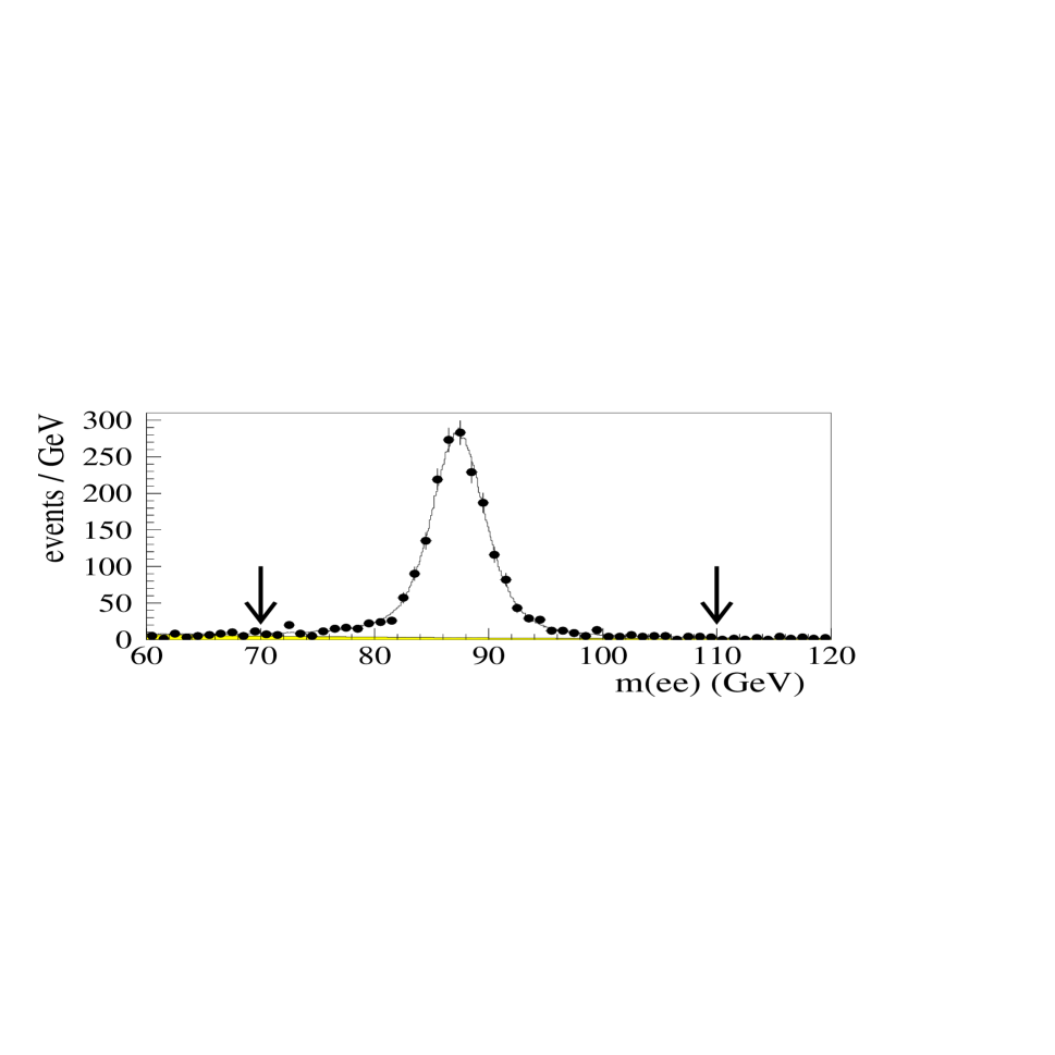
FIG. 1.: The dielectron invariant mass distribution of the $Z$ data for sample II ($\bullet$). The solid line shows the fitted signal plus background shape and the small shaded area the background. The arrows indicate the fit window.

FIG. 2.: The definition of the $\eta$-axis (left). The plot of $u_{\eta}/{\rm R_{rec}}+p_{\eta}(ee)$ (right) for the data ($\bullet$) and simulation (—).

FIG. 3.: Spectra of (a) $m_{T}$ and (b) $p_{T}(e)$ from the data ($\bullet$), the fit (—), and the backgrounds (shaded). The arrows indicate the fit windows.

REFERENCES

- [1] Visitor from Universidad San Francisco de Quito, Quito, Ecuador.
- [2] Visitor from IHEP, Beijing, China.
- [3] S.L. Glashow, Nucl. Phys. 22, 579 (1961); S. Weinberg, Phys. Rev. Lett. 19, 1264 (1967); A. Salam, Proceedings of the 8th Nobel Symposium, edited by N. Svartholm (Almqvist and Wiksells, Stockholm 1968), p. 367.
- [4] A. Sirlin, Phys. Rev. D 22, 971 (1980); W. Marciano and A. Sirlin, Phys. Rev. D 22, 2695 (1980) and erratum-ibid. 31, 213 (1985).
- [5] S. Abachi et al. (DØ Collaboration), Nucl. Instrum. Methods in Phys. Res. A 338, 185 (1994).
- [6] I. Adam, Ph.D. thesis, Columbia University, 1997, Nevis Report #294 (unpublished), http://www-d0.fnal.gov/publications_talks/thesis/adam/ian_thesis_all.ps.
- [7] E. Flattum, Ph.D. thesis, Michigan State University, 1996 (unpublished), http://www-d0.fnal.gov/publications_talks/thesis/flattum/eric_thesis.ps.
- [8] B. Abbott et al. (DØ Collaboration), FERMILAB-PUB-97/422-E (1997), submitted to Phys. Rev. D.
- [9] J. Alitti et al. (UA2 Collaboration), Phys. Lett. B 276, 354 (1992).
- [10] F. Abe et al. (CDF Collaboration), Phys. Rev. Lett. 75, 11 (1995) and Phys. Rev. D 52, 4784 (1995).
- [11] S. Abachi et al. (DØ Collaboration), Phys. Rev. Lett. 77, 3309 (1996); B. Abbott et al. (DØ Collaboration), FERMILAB-PUB-97/328-E, submitted to Phys. Rev. D.
- [12] K. Ackerstaff et al. (OPAL Collaboration), Phys. Lett. B 389, 416 (1996).
- [13] P. Abreu et al. (Delphi Collaboration), Phys. Lett. B 397, 158 (1997).
- [14] M. Acciarri et al. (L3 Collaboration), Phys. Lett. B 398, 223 (1997).
- [15] R. Barate et al. (ALEPH Collaboration), Phys. Lett. B 401, 347 (1997).
- [16] We generically refer to electrons and positrons as electrons.
- [17] We define the pseudorapidity .
- [18] G.A. Ladinsky and C.-P. Yuan, Phys. Rev. D 50, 4239 (1994).
- [19] A.D. Martin, W.J. Stirling, and R.G. Roberts, Phys. Rev. D 50, 6734 (1994) and ibid. 51, 4756 (1995).
- [20] S. Abachi et al. (DØ Collaboration), Phys. Rev. Lett. 75, 1456 (1995).
- [21] The LEP Collaborations, the LEP Electroweak Working Group, and the SLD Heavy Flavour Group, CERN-PPE/96-183 (unpublished).
- [22] E. Mirkes, Nucl. Phys. B387, 3 (1992).
- [23] F.A. Berends and R. Kleiss, Z. Phys. C 27, 365 (1985).
- [24] R.M. Barnett et al., Phys. Rev. D 54, 1 (1996).
- [25] F. Carminati et al., geantUsers Guide, CERN Program Library W5013, 1991 (unpublished).
- [26] A.D. Martin, W.J. Stirling, and R.G. Roberts, Phys. Lett. B 306, 145 (1993) and erratum-ibid. 309, 492 (1993).
- [27] J. Botts et al., Phys. Lett. B 304, 159 (1993).
- [28] H.L. Lai et al., Phys. Rev. D 51, 4763 (1995).
- [29] U. Baur et al., Phys. Rev. D 56, 140 (1997) and references therein.