A Measurement of the $W$ Boson Mass

Abstract

We present a measurement of the $W$ boson mass using data collected by the DØ experiment at the Fermilab Tevatron during 1994–1995. We identify $W$ bosons by their decays to $e\nu$ final states. We extract the $W$ mass, $M_{W}$, by fitting the transverse mass and transverse electron momentum spectra from a sample of 28,323 $W\to e\nu$ decay candidates. We use a sample of 3,563 dielectron events, mostly due to $Z\to ee$ decays, to constrain our model of the detector response. From the transverse mass fit we measure $M_{W}=80.44\pm 0.10(stat)\pm 0.07(syst)$ GeV. Combining this with our previously published result from data taken in 1992–1993, we obtain $M_{W}=80.43\pm 0.11$ GeV.

I Introduction

In this article we describe the most precise measurement to date of the mass of the $W$ boson, using data collected in 1994–1995 with the DØ detector at the Fermilab Tevatron $p\overline{p}$ collider [1, 2, 3].

The study of the properties of the $W$ boson began in 1983 with its discovery by the UA1 [4] and UA2 [5] collaborations at the CERN $p\overline{p}$ collider. Together with the discovery of the $Z$ boson in the same year [6, 7], it provided a direct confirmation of the unified model of the weak and electromagnetic interactions [8], which – together with QCD – is now called the Standard Model.

Since the $W$ and $Z$ bosons are carriers of the weak force, their properties are intimately coupled to the structure of the model. The properties of the $Z$ boson have been studied in great detail in $e^{+}e^{-}$ collisions [9]. The study of the $W$ boson has proven to be significantly more difficult, since it is charged and therefore can not be resonantly produced in $e^{+}e^{-}$ collisions. Until recently its direct study has therefore been the realm of experiments at $p\overline{p}$ colliders which have performed the most precise direct measurements of the $W$ boson mass [10, 11, 12]. Direct measurements of the $W$ boson mass have also been carried out at LEP2 [13, 14, 15, 16] using nonresonant $W$ pair production. A summary of these measurements can be found in Table XV at the end of this article.

The Standard Model links the $W$ boson mass to other parameters,

$$M_{W}=\left({\pi\alpha\over\sqrt{2}G_{F}}\right)^{1\over 2}{1\over\sin\theta_{W}\sqrt{1-\Delta r}}.$$ (1)

In the “on shell” scheme [17]

$$\cos\theta_{W}={M_{W}\over M_{Z}},$$ (2)

where $\theta_{W}$ is the weak mixing angle. Aside from the radiative corrections $\Delta r$, the $W$ boson mass is thus determined by three precisely measured quantities, the mass of the $Z$ boson $M_{Z}$[9], the Fermi constant $G_{F}$ [18] and the electromagnetic coupling constant $\alpha$ evaluated at $Q^{2}=M_{Z}^{2}$ [19]:

$$M_{Z} = 91.1865\pm 0.0020\ \hbox{GeV},$$ (3)

$$G_{F} = (1.16639\pm 0.00002)\times 10^{-5}\ \hbox{GeV}^{-2},$$ (4)

$$\alpha = (128.896\pm 0.090)^{-1}.$$ (5)

From the measured $W$ boson mass we can derive the size of the radiative corrections $\Delta r$. Within the framework of the Standard Model, these corrections are dominated by loops involving the top quark and the Higgs boson (see Fig. 1). The correction from the $t\overline{b}$ loop is substantial because of the large mass difference between the two quarks. It is proportional to $m_{t}^{2}$ for large values of the top quark mass $m_{t}$. Since $m_{t}$ has been measured [20], this contribution can be calculated within the Standard Model. For a large Higgs boson mass, $m_{H}$, the correction from the Higgs loop is proportional to $\ln m_{H}$. In extensions to the Standard Model new particles may give rise to additional corrections to the value of $M_{W}$. In the Minimal Supersymmetric extension of the Standard Model (MSSM), for example, additional corrections can increase the predicted $W$ mass by up to 250 MeV [21].

A measurement of the $W$ boson mass therefore constitutes a test of the Standard Model. In conjunction with a measurement of the top quark mass the Standard Model predicts $M_{W}$ up to a 200 MeV uncertainty due to the unknown Higgs boson mass. By comparing with the measured value of the $W$ boson mass we can constrain the mass of the Higgs boson, the agent of the electroweak symmetry breaking that has up to now eluded experimental detection. A discrepancy with the range allowed by the Standard Model could indicate new physics. The experimental challenge is thus to measure the $W$ boson mass to sufficient precision, about 0.1%, to be sensitive to these corrections.

II Overview

A Conventions

We use a Cartesian coordinate system with the $z$-axis defined by the direction of the proton beam, the $x$-axis pointing radially out of the Tevatron ring and the $y$-axis pointing up. A vector $\vec{p}$ is then defined in terms of its projections on these three axes, $p_{x}$, $p_{y}$, $p_{z}$. Since protons and antiprotons in the Tevatron are unpolarized, all physical processes are invariant with respect to rotations around the beam direction. It is therefore convenient to use a cylindrical coordinate system, in which the same vector is given by the magnitude of its component transverse to the beam direction, $p_{T}$, its azimuth $\phi$, and $p_{z}$. In $p\overline{p}$ collisions the center of mass frame of the parton-parton collisions is approximately at rest in the plane transverse to the beam direction but has an undetermined motion along the beam direction. Therefore the plane transverse to the beam direction is of special importance and sometimes we work with two-dimensional vectors defined in the $x$-$y$ plane. They are written with a subscript $T$, e.g. $\vec{p}_{T}$. We also use spherical coordinates by replacing $p_{z}$ with the colatitude $\theta$ or the pseudorapidity $\eta=-\ln\tan\left(\theta/2\right)$. The origin of the coordinate system is in general the reconstructed position of the $p\overline{p}$ interaction when describing the interaction, and the geometrical center of the detector when describing the detector. For convenience, we use units in which $c=\hbar=1$.

B $W$ and $Z$ Boson Production and Decay

In $p\overline{p}$ collisions at $\sqrt{s}=1.8$ TeV, $W$ and $Z$ bosons are produced predominantly through quark-antiquark annihilation. Figure 2 shows the lowest-order diagrams. The quarks in the initial state may radiate gluons which are usually very soft but may sometimes be energetic enough to give rise to hadron jets in the detector. In the reaction the initial proton and antiproton break up and the fragments hadronize. We refer to everything except the vector boson and its decay products collectively as the underlying event. Since the initial proton and antiproton momentum vectors add to zero, the same must be true for the vector sum of all final state momenta and therefore the vector boson recoils against all particles in the underlying event. The sum of the transverse momenta of the recoiling particles must balance the transverse momentum of the boson, which is typically small compared to its mass but has a long tail to large values.

We identify $W$ and $Z$ bosons by their leptonic decays. The DØ detector (Sec. III) is best suited for a precision measurement of electrons and positrons, and we therefore use the decay channel $W\to e\nu$ to measure the $W$ boson mass. $Z\to ee$ decays serve as an important calibration sample. About 11% of the $W$ bosons decay to $e\nu$ and about 3.3% of the $Z$ bosons decay to $ee$. The leptons typically have transverse momenta of about half the mass of the decaying boson and are well isolated from other large energy deposits in the calorimeter. Intermediate vector boson decays are the dominant source of isolated high-$p_{T}$ leptons at the Tevatron, and therefore these decays allow us to select a clean sample of $W$ and $Z$ boson decays.

C Event Characteristics

In events due to the process $p\overline{p}\to(W\to e\nu)+X$, where $X$ stands for the underlying event, we detect the electron and all particles recoiling against the $W$ with pseudorapidity $-4<\eta<4$. The neutrino escapes undetected. In the calorimeter we cannot resolve individual recoil particles, but we measure their energies summed over detector segments. Recoil particles with $|\eta|>4$ escape unmeasured through the beampipe, possibly carrying away substantial momentum along the beam direction. This means that we cannot measure the sum of the $z$-components of the recoil momenta, $u_{z}$, precisely. Since these particles escape at a very small angle with respect to the beam, their transverse momenta are typically small and can be neglected in the sum of the transverse recoil momenta, $\vec{u}_{T}$. We measure $\vec{u}_{T}$ by summing the observed energy flow vectorially over all detector segments. Thus, we reduce the reconstruction of every candidate event to a measurement of the electron momentum $\vec{p}(e)$ and $\vec{u}_{T}$.

Since the neutrino escapes undetected, the sum of all measured final state transverse momenta does not add to zero. The missing transverse momentum $\hbox to0.0pt{\kern 1.00006pt/\hss}\vec{p}_{T}$, required to balance the transverse momentum sum, is a measure of the transverse momentum of the neutrino. The neutrino momentum component along the beam direction cannot be determined, because $u_{z}$ is not measured well. The signature of a $W\to e\nu$ decay is therefore an isolated high-$p_{T}$ electron and large missing transverse momentum.

In the case of $Z\to ee$ decays the signature consists of two isolated high-$p_{T}$ electrons and we measure the momenta of both leptons, $\vec{p}(e_{1})$ and $\vec{p}(e_{2})$, and $\vec{u}_{T}$ in the detector.

D Mass Measurement Strategy

Since $p_{z}(\nu)$ is unknown, we cannot reconstruct the $e\nu$ invariant mass for $W\to e\nu$ candidate events and therefore must resort to other kinematic variables for the mass measurement.

For recent measurements [10, 11, 12] the transverse mass,

$$m_{T}=\sqrt{2p_{T}(e)p_{T}(\nu)\left(1-\cos\left(\phi(e)-\phi(\nu)\right)\right)}$$ (6)

was used. This variable has the advantage that its spectrum is relatively insensitive to the production dynamics of the $W$. Corrections to $m_{T}$ due to the motion of the $W$ are of order $\left(q_{T}/M_{W}\right)^{2}$, where $q_{T}$ is the transverse momentum of the $W$ boson. It is also insensitive to selection biases that prefer certain event topologies (Sec. VI C). However, it makes use of the inferred neutrino $p_{T}$ and is therefore sensitive to the response of the detector to the recoil particles.

The electron $p_{T}$ spectrum provides an alternative measurement of the $W$ mass. It is measured with better resolution than the neutrino $p_{T}$ and is insensitive to the recoil momentum measurement. However, its shape is sensitive to the motion of the $W$ and receives corrections of order $q_{T}/M_{W}$. It thus requires a better understanding of the $W$ boson production dynamics than the $m_{T}$ spectrum.

The $m_{T}$ and $p_{T}(e)$ spectra thus provide us with two complementary measurements. This is illustrated in Figs. 3 and 4, which show the effect of the motion of the $W$ bosons and the detector resolutions on the shape of each of the two spectra. The solid line shows the shape of the distribution before the detector simulation and with $q_{T}$=0. The points show the shape after $q_{T}$ is added to the system, and the shaded histogram also includes the detector simulation. We observe that the shape of the $m_{T}$ spectrum is dominated by detector resolutions and the shape of the $p_{T}(e)$ spectrum by the motion of the $W$. By performing the measurement using both spectra we provide a powerful cross-check with complementary systematics.

Both spectra are equally sensitive to the electron energy response of the detector. We calibrate this response by forcing the observed dielectron mass peak in the $Z\to ee$ sample to agree with the known $Z$ mass[9] (Sec. VI). This means that we effectively measure the ratio of $W$ and $Z$ masses, which is equivalent to a measurement of the $W$ mass because the $Z$ mass is known precisely.

To carry out these measurements we perform a maximum likelihood fit to the spectra. Since the shape of the spectra, including all the experimental effects, cannot be computed analytically, we need a Monte Carlo simulation program that can predict the shape of the spectra as a function of the $W$ mass. To perform a measurement of the $W$ mass to a precision of order 100 MeV we have to estimate individual systematic effects to 10 MeV. This requires a Monte Carlo sample of 2.5 million accepted $W$ bosons for each such effect. The program therefore must be capable of generating large samples in a reasonable time. We achieve the required performance by employing a parameterized model of the detector response.

We next summarize the aspects of the accelerator and detector that are important for our measurement (Sec. III). Then we describe the data selection (Sec. IV) and the fast Monte Carlo model (Sec. V). Most parameters in the model are determined from our data. We describe the determination of the various components of the Monte Carlo model in Secs. VI-IX. After tuning the model we fit the kinematic spectra (Sec. X), perform some consistency checks (Sec. XI), and discuss the systematic uncertainties (Sec. XII). Section XIII summarizes the results and presents the conclusions.

III Experimental Setup

A Accelerator

The Fermilab Tevatron[22] collides proton and antiproton beams at a center-of-mass energy of $\sqrt{s}=1.8$ TeV. Six bunches each of protons and antiprotons circulate around the ring in opposite directions. Bunches cross at the intersection regions every 3.5 $\mu$s. During the 1994–1995 running period, the accelerator reached a peak luminosity of $2.5\times 10^{31}\hbox{cm}^{-2}\hbox{s}^{-1}$ and delivered an integrated luminosity of about 100 pb^-1.

The Tevatron tunnel also houses a 150 GeV proton synchrotron, called the Main Ring, which is used as an injector for the Tevatron. The Main Ring also serves to accelerate protons for antiproton production during collider operation. Since the Main Ring beampipe passes through the outer section of the DØ calorimeter, passing proton bunches give rise to backgrounds in the detector. We eliminate this background using timing cuts based on the accelerator clock signal.

B Detector

1 Overview

The DØ detector consists of three major subsystems: a central detector, a calorimeter (Fig. 5), and a muon spectrometer. It is described in detail in Ref. [23]. We describe only the features that are most important for this measurement.

2 Central Detector

The central detector is designed to measure the trajectories of charged particles. It consists of a vertex drift chamber, a transition radiation detector, a central drift chamber (CDC), and two forward drift chambers (FDC). There is no central magnetic field. The CDC covers the region $|\eta|<1.0$. It is a jet-type drift chamber with delay lines to give the hit coordinates in the $r$-$z$ plane. The FDC covers the region $1.4<|\eta|<3.0$.

3 Calorimeter

The calorimeter is the most important part of the detector for this measurement. It is a sampling calorimeter and uses uranium absorber plates and liquid argon as the active medium. It is divided into three parts: a central calorimeter (CC) and two end calorimeters (EC), each housed in its own cryostat. Each is segmented into an electromagnetic (EM) section, a fine hadronic (FH) section, and a coarse hadronic (CH) section, with increasingly coarser sampling. The CC-EM section is constructed of 32 azimuthal modules. The entire calorimeter is divided into about 5000 pseudo-projective towers, each covering 0.1$\times$0.1 in $\eta\times\phi$. The EM section is segmented into four layers, 2, 2, 7, and 10 radiation lengths thick. The third layer, in which electromagnetic showers typically reach their maximum, is transversely segmented into cells covering 0.05$\times$0.05 in $\eta\times\phi$. The hadronic section is segmented into four layers (CC) or five layers (EC). The entire calorimeter is 7–9 nuclear interaction lengths thick. There are no projective cracks in the calorimeter and it provides hermetic and almost uniform coverage for particles with $|\eta|<4$. Figure 5 shows a view of the calorimeter and the central detector.

The signals from arrays of 2$\times$2 calorimeter towers, covering 0.2$\times$0.2 in $\eta\times\phi$, are added together electronically for the EM section only and for all sections, and shaped with a fast rise time for use in the Level 1 trigger. We refer to these arrays of 2$\times$2 calorimeter towers as “trigger towers”.

Figure 6 shows the pedestal spectrum of a calorimeter cell. The spectrum has an asymmetric tail from ionization caused by the intrinsic radioactivity of the uranium absorber plates. The data are corrected such that the mean pedestal is zero for each cell. To reduce the amount of data that have to be stored, the calorimeter readout is zero-suppressed. Only cells with a signal that deviates from zero by more than twice the rms of the pedestal distribution are read out. This region of the pedestal spectrum is indicated by the shaded region in Fig. 6. Due to its asymmetry, the spectrum does not average to zero after zero-suppression. Thus the zero-suppression effectively causes a pedestal shift.

The liquid argon has unit gain and therefore the calorimeter response was extremely stable during the entire run. Figure 7 shows the response of the liquid argon as monitored with radioactive sources of $\alpha$ and $\beta$ particles. Figures 8 and 9 show the gains and pedestals of a typical readout channel throughout the run.

The EM calorimeter provides a measurement of energy and position of the electrons from the $W$ and $Z$ decays. Due to the fine segmentation of the third layer, we can measure the position of the shower centroid with a precision of 2.5 mm in the azimuthal direction and 1 cm in the $z$-direction.

We study the response of the EM calorimeter to electrons in beam tests [24]. To reconstruct the electron energy we add the signals $a_{i}$ observed in each EM layer ($i=1\ldots 4$) and the first FH layer ($i=5$) of an array of 5$\times$5 calorimeter towers, centered on the most energetic tower, weighted by a layer dependent sampling weight $s_{i}$,

$$E=A\sum_{i=1}^{5}s_{i}a_{i}-\delta_{\rm EM}.$$ (7)

To determine the sampling weights we minimize

$$\chi^{2}=\sum{(p_{\rm beam}-E)\over\sigma_{\rm EM}^{2}},$$ (8)

where the sum runs over all events and $\sigma_{\rm EM}$ is the resolution given in Eq. 9. We obtain $A=2.96$ MeV/ADC count, $\delta_{\rm EM}=-347$ MeV, $s_{1}=1.31$, $s_{2}=0.85$, $s_{4}=0.98$, and $s_{5}=1.84$. We arbitrarily fix $s_{3}=1$. The value of $\delta_{\rm EM}$ depends on the amount of dead material in front of the calorimeter. The parameters $s_{1}$ to $s_{4}$ weight the four EM layers and $s_{5}$ the first FH layer. Figure 10 shows the fractional deviation of $E$ as a function of the beam momentum $p_{\rm beam}$. Above 10 GeV they deviate by less than 0.3% from each other.

The fractional energy resolution can be parameterized as a function of electron energy using constant, sampling, and noise terms as

$$\left({\sigma_{\rm EM}\over E}\right)^{2}=c_{\rm EM}^{2}+\left({s_{\rm EM}\over\sqrt{E\sin\theta}}\right)^{2}+\left({n_{\rm EM}\over E}\right)^{2}$$ (9)

with $c_{\rm EM}=0.003$, $s_{\rm EM}=0.135$ GeV^1/2 [25, 26], and $n_{\rm EM}=0.43$ GeV in the central calorimeter. The angle $\theta$ is the colatitude of the electron. Figure 11 shows the fractional electron energy resolution versus beam momentum for a CC-EM module. The line shows the parametrization of the resolution from Eq. 9.

4 Luminosity Monitor

Two arrays of scintillator hodoscopes, mounted in front of the EC cryostats, register hits with a 220 ps time resolution. They serve to detect that an inelastic $p\overline{p}$ interaction has taken place. The particles from the breakup of the proton give rise to hits in the hodoscopes on one side of the detector that are tightly clustered in time. The detector has a 91% acceptance for inelastic $p\overline{p}$ interactions. For events with a single interaction the location of the interaction vertex can be determined with a resolution of 3 cm from the time difference between the hits on the two sides of the detector for use in the Level 2 trigger. This array is also called the Level 0 trigger because the detection of an inelastic $p\overline{p}$ interaction is a basic requirement of most trigger conditions.

5 Trigger

Readout of the detector is controlled by a two-level trigger system.

Level 1 consists of an and-or network, that can be programmed to trigger on a $p\overline{p}$ crossing if a number of preselected conditions are true. The Level 1 trigger decision is taken within the 3.5 $\mu$s time interval between crossings. As an extension to Level 1, a trigger processor (Level 1.5) may be invoked to execute simple algorithms on the limited information available at the time of a Level 1 accept. For electrons, the processor uses the energy deposits in each trigger tower as inputs. The detector cannot accept any triggers until the Level 1.5 processor completes execution and accepts or rejects the event.

Level 2 of the trigger consists of a farm of 48 VAXstation 4000’s. At this level the complete event is available. More sophisticated algorithms refine the trigger decisions and events are accepted based on preprogrammed conditions. Events accepted by Level 2 are written to magnetic tape for offline reconstruction.

IV Data Selection

A Trigger

The conditions required at trigger Level 1 for $W$ and $Z$ candidates are:

• $\underline{\hbox{$p\overline{p}$\ interaction:}}$ Level 0 hodoscopes register hits consistent with a $p\overline{p}$ interaction. This condition accepts 98.6% of all $W$ and $Z$ bosons produced.

• $\underline{\hbox{Main Ring Veto:}}$ No Main Ring proton bunch passes through the detector less than 800 ns before or after the $p\overline{p}$ crossing and no protons were injected into the Main Ring less than 400 ms before the $p\overline{p}$ crossing.

• $\underline{\hbox{EM trigger towers:}}$ There are one or more EM trigger towers with $E\sin\theta>T$, where $E$ is the energy measured in the tower, $\theta$ its angle with the beam measured from the center of the detector, and $T$ a programmable threshold. This requirement is fully efficient for electrons with $p_{T}>2T$.

The Level 1.5 processor recomputes the transverse electron energy by adding the adjacent EM trigger tower with the largest signal to the EM trigger tower that exceeded the Level 1 threshold. In addition, the signal in the EM trigger tower that exceeded the Level 1 threshold must constitute at least 85% of the signal registered in this tower if the hadronic layers are also included. This EM fraction requirement is fully efficient for electron candidates that pass our offline selection (Sec. IV D).

Level 2 uses the EM trigger tower that exceeded the Level 1 threshold as a starting point. The Level 2 algorithm finds the most energetic of the four calorimeter towers that make up the trigger tower, and sums the energy in the EM sections of a 3$\times$3 array of calorimeter towers around it. It checks the longitudinal shower shape by applying cuts on the fraction of the energy in the different EM layers. The transverse shower shape is characterized by the energy deposition pattern in the third EM layer. The difference between the energies in concentric regions covering 0.25$\times$0.25 and 0.15$\times$0.15 in $\eta\times\phi$ must be consistent with an electron. Level 2 also imposes an isolation condition requiring

$$\frac{\sum_{i}E_{i}\sin\phi_{i}-p_{T}}{p_{T}}<0.15$$ (10)

where the sum runs over all cells within a cone of radius $R=\sqrt{\Delta\phi^{2}+\Delta\eta^{2}}=0.4$ around the electron direction and $p_{T}$ is the transverse momentum of the electron [27].

The $p_{T}$ of the electron computed at Level 2 is based on its energy and the $z$-position of the interaction vertex measured by the Level 0 hodoscopes. Level 2 accepts events that have a minimum number of EM clusters that satisfy the shape cuts and have $p_{T}$ above a preprogrammed threshold. Figure 12 shows the measured relative efficiency of the Level 2 electron filter versus electron $p_{T}$ for a Level 2 $p_{T}$ threshold of 20 GeV. We determine this efficiency using $Z$ data taken with a lower threshold value (16 GeV). The efficiency is the fraction of electrons above a Level 2 $p_{T}$ threshold of 20 GeV. The curve is the parameterization used in the fast Monte Carlo.

Level 2 also computes the missing transverse momentum based on the energy registered in each calorimeter cell and the vertex $z$-position. We determine the efficiency curve for a 15 GeV Level 2 $\hbox to0.0pt{\kern 1.00006pt/\hss}p_{T}$ requirement from data taken without the Level 2 $\hbox to0.0pt{\kern 1.00006pt/\hss}p_{T}$ condition. Figure 13 shows the measured efficiency versus $p_{T}(\nu)$. The curve is the parameterization used in the fast Monte Carlo.

B Reconstruction

1 Electron

We identify electrons as clusters of adjacent calorimeter cells with significant energy deposits. Only clusters with at least 90% of their energy in the EM section and at least 60% of their energy in the most energetic calorimeter tower are considered as electron candidates. For most electrons we also reconstruct a track in the CDC or FDC that points towards the centroid of the cluster.

We compute the electron energy $E(e)$ from the signals in all cells of the EM layers and the first FH layer in a window covering 0.5$\times$0.5 in $\eta\times\phi$ and centered on the tower which registered the highest fraction of the electron energy. In the computation we use the sampling weights and calibration constants determined using the testbeam data (Sec. III B 3) except for the offset $\delta_{\rm EM}$, which we take from an in situ calibration (Sec. VI D), i.e. $\delta_{\rm EM}=-0.16$ GeV for electrons in the CC.

The calorimeter shower centroid position ($x_{\rm cal}$, $y_{\rm cal}$, $z_{\rm cal}$), the center of gravity of the track ($x_{\rm trk}$, $y_{\rm trk}$, $z_{\rm trk}$) and the proton beam trajectory define the electron direction. The shower centroid algorithm is documented in Appendix B. The center of gravity of the CDC track is defined by the mean hit coordinates of all the delay line hits on the track. The calibration of the measured $z$-coordinates contributes a significant systematic uncertainty to the $W$ boson mass measurement and is described in Appendices A and B. Using tracks from many events reconstructed in the vertex drift chamber, we measure the beam trajectory for every run. The closest approach to the beam trajectory of the line through shower centroid and track center of gravity defines the position of the interaction vertex ($x_{\rm vtx}$, $y_{\rm vtx}$, $z_{\rm vtx}$). In $Z\to ee$ events we may have two electron candidates with tracks. In this case we take the point midway between the vertex positions determined from each electron as the interaction vertex. Using only the electron track to determine the position of the interaction vertex, rather than all tracks in the event, makes the resolution of this measurement less sensitive to the luminosity and avoids confusion between vertices in events with more than one $p\overline{p}$ interaction.

We then define the azimuth $\phi(e)$ and the colatitude $\theta(e)$ of the electron using the vertex and the shower centroid positions,

$$\tan\phi(e) = {y_{\rm cal}-y_{\rm vtx}\over x_{\rm cal}-x_{\rm vtx}},$$ (11)

$$\tan\theta(e) = {\sqrt{x_{\rm cal}^{2}+y_{\rm cal}^{2}}-\sqrt{x_{\rm vtx}^{2}+y_{\rm vtx}^{2}}\over z_{\rm cal}-z_{\rm vtx}}.$$ (12)

Neglecting the electron mass, the momentum of the electron is given by

$$\vec{p}(e)=E(e)\left(\begin{array}[]{l}\sin\theta(e)\cos\phi(e)\\ \sin\theta(e)\sin\phi(e)\\ \cos\theta(e)\end{array}\right).$$ (13)

2 Recoil

We reconstruct the transverse momentum of all particles recoiling against the $W$ or $Z$ boson by taking the vector sum

$$\vec{u}_{T}=\sum_{i}E_{i}\sin\theta_{i}\left(\begin{array}[]{c}\cos\phi_{i}\\ \sin\phi_{i}\end{array}\right),$$ (14)

where the sum runs over all calorimeter cells that were read out, except those that belong to electron clusters. $E_{i}$ are the cell energies, and $\phi_{i}$ and $\theta_{i}$ are the azimuth and colatitude of the center of cell $i$ with respect to the interaction vertex.

3 Derived Quantities

In the case of $Z\to ee$ decays we define the dielectron momentum

$$\vec{p}(ee)=\vec{p}(e_{1})+\vec{p}(e_{2})$$ (15)

and the dielectron invariant mass

$$m(ee)=\sqrt{2E(e_{1})E(e_{2})(1-\cos\omega)},$$ (16)

where $\omega$ is the opening angle between the two electrons. It is useful to define a coordinate system in the plane transverse to the beam that depends only on the electron directions. We follow the conventions first introduced by UA2[10] and call the axis along the inner bisector of the two electrons the $\eta$-axis and the axis perpendicular to that the $\xi$-axis. Projections on these axes are denoted with subscripts $\eta$ or $\xi$. Figure 14 illustrates these definitions.

In case of $W\to e\nu$ decays we define the transverse neutrino momentum

$$\vec{p}_{T}(\nu)=-\vec{p}_{T}(e)-\vec{u}_{T}$$ (17)

and the transverse mass (Eq. 6). Useful quantities are the projection of the transverse recoil momentum on the electron direction,

$$u_{\parallel}=\vec{u}_{T}\cdot\hat{p}_{T}(e),$$ (18)

and the projection on the direction perpendicular to the electron direction,

$$u_{\perp}=\vec{u}_{T}\cdot(\hat{p}_{T}(e)\times\hat{z}).$$ (19)

Figure 15 illustrates these definitions.

C Electron Identification

1 Fiducial Cuts

To ensure a uniform response we accept only electron candidates that are well separated in azimuth ($\Delta\phi$) from the calorimeter module boundaries in the CC-EM and from the edges of the calorimeter by cutting on $\Delta\phi$ and $z_{\rm cal}$. We also remove electrons for which the $z$-position of the track center of gravity is near the edge of the CDC. For electrons in the EC-EM we cut on the index of the most energetic tower, $i_{\eta}$. Tower 15 covers $1.4<\eta<1.5$ with respect to the detector center and tower 25 covers $2.4<\eta<2.5$.

2 Quality Variables

We test how well the shape of a cluster agrees with that expected for an electromagnetic shower by computing a quality variable ($\chi^{2}$) for all cell energies using a 41-dimensional covariance matrix. The covariance matrix was determined from geant [28] based simulations [29].

To determine how well a track matches a cluster we extrapolate the track to the third EM layer in the calorimeter and compute the distance between the extrapolated track and the cluster centroid in the azimuthal direction, $\Delta s$, and in the $z$-direction, $\Delta z$. The variable

$$\sigma_{\rm trk}^{2}=\left({\Delta s\over\delta s}\right)^{2}+\left({\Delta z\over\delta z}\right)^{2},$$ (20)

quantifies the quality of the match. In the EC-EM $z$ is replaced by $r$, the radial distance from the center of the detector. The parameters $\delta s=0.25$ cm, $\delta z=2.1$ cm, and $\delta r=1.0$ cm are the resolutions with which $\Delta s$, $\Delta z$, and $\Delta r$ are measured, as determined with the electrons from $W\to e\nu$ decays.

In the EC, electrons must have a matched track in the forward drift chamber. In the CC, we define “tight” and “loose” criteria. The tight criteria require a matched track in the CDC. The loose criteria do not require a matched track and help increase the electron finding efficiency for $Z\to ee$ decays.

The isolation fraction is defined as

$$f_{\rm iso}={E_{\rm cone}-E_{\rm core}\over E_{\rm core}},$$ (21)

where $E_{\rm cone}$ is the energy in a cone of radius $R=\sqrt{\Delta\phi^{2}+\Delta\eta^{2}}=0.4$ around the direction of the electron, summed over the entire depth of the calorimeter and $E_{\rm core}$ is the energy in a cone of $R=0.2$, summed over the EM calorimeter only.

Figure 16 shows the distributions of the three quality variables for electrons in the CC with the arrow showing the cut values. Table I summarizes the electron selection criteria.

D Data Samples

The data were taken during the 1994–1995 Tevatron run. After the removal of runs in which parts of the detector were not operating adequately, they amount to an integrated luminosity of about 82 pb^-1. We select $W$ decay candidates by requiring:

Level 1:	$p\overline{p}$ interaction
	Main Ring Veto
	EM trigger tower above 10 GeV
Level 1.5:	$\geq 1$ EM cluster above 15 GeV
Level 2:	electron candidate with $p_{T}>20$ GeV
	momentum imbalance $\mbox{$\hbox to0.0pt{\kern 1.00006pt/\hss}p_{T}$}>15$ GeV
offline:	$\geq 1$ tight electron candidate in CC
	$p_{T}(e)>25$ GeV
	$p_{T}(\nu)>25$ GeV
	$u_{T}<15$ GeV

We select $Z$ decay candidates by requiring:

Level 1:	$p\overline{p}$ interaction
	$\geq 2$ EM trigger towers above 7 GeV
Level 1.5:	$\geq 1$ EM cluster above 10 GeV
Level 2:	$\geq 2$ electron candidates with $p_{T}>20$ GeV
offline:	$\geq 2$ electron candidates
	$p_{T}(e)>25$ GeV
	$70<m(ee)<110$ GeV

We accept $Z\to ee$ decays with at least one electron candidate in the CC and the other in the CC or the EC. One CC candidate must pass the tight electron selection criteria. If the other candidate is also in the CC it may pass only the loose criteria. We use the 2,179 events with both electrons in the CC (CC/CC $Z$ sample) to calibrate the calorimeter response to electrons (Sec. VI). These events need not pass the Main Ring Veto cut because Main Ring background does not affect the EM calorimeter. The 2,341 events for which both electrons have tracks and which pass the Main Ring Veto (CC/CC+EC $Z$ sample) serve to calibrate the recoil momentum response (Sec. VII). Table II summarizes the data samples.

Figure 17 shows the luminosity of the colliding beams during the $W$ and $Z$ data collection.

On several occasions we use a sample of 295,000 random $p\overline{p}$ interaction events for calibration purposes. We collected these data concurrently with the $W$ and $Z$ signal data, requiring only a $p\overline{p}$ interaction at Level 1. We refer to these data as “minimum bias events”.

V Fast Monte Carlo Model

A Overview

The fast Monte Carlo model consists of three parts. First we simulate the production of the $W$ or $Z$ boson by generating the boson four-momentum and other characteristics of the event like the $z$-position of the interaction vertex and the luminosity. The event luminosity is required for luminosity dependent parametrizations in the detector simulation. Then we simulate the decay of the boson. At this point we know the true $p_{T}$ of the boson and the momenta of its decay products. We then apply a parameterized detector model to these momenta in order to simulate the observed transverse recoil momentum and the observed electron momenta.

B Vector Boson Production

In order to specify completely the production dynamics of vector bosons in $p\overline{p}$ collisions we need to know the differential production cross section in mass $Q$, rapidity $y$, and transverse momentum $q_{T}$ of the produced $W$ bosons. To speed up the event generation, we factorize this into

$${\mbox{d}^{3}\sigma\over\mbox{d}q_{T}^{2}\mbox{d}y\mbox{d}Q}\approx\left.{\mbox{d}^{2}\sigma\over\mbox{d}q_{T}^{2}\mbox{d}y}\right|_{Q^{2}=M_{W}^{2}}\times{\mbox{d}\sigma\over\mbox{d}Q}$$ (22)

to generate $q_{T}$, $y$, and $Q$ of the bosons.

For $p\overline{p}$ collisions, the vector boson production cross section is given by the parton cross section $\widetilde{\sigma}_{i,j}$ convoluted with the parton distribution functions $f(x,Q^{2})$ and summed over parton flavors $i,j$:

$${\mbox{d}^{2}\sigma\over\mbox{d}q_{T}^{2}\mbox{d}y} = \sum_{i,j}\int dx_{1}\int dx_{2}f_{i}(x_{1},Q^{2})f_{j}(x_{2},Q^{2})$$ (24)

$$\ \ \delta(sx_{1}x_{2}-Q^{2}){\mbox{d}^{2}\widetilde{\sigma}_{i,j}\over\mbox{d}q_{T}^{2}\mbox{d}y}.$$

Several authors [30, 31] have computed $\left.{\mbox{d}^{2}\sigma\over\mbox{d}q_{T}^{2}\mbox{d}y}\right|_{Q^{2}=M_{W}^{2}}$ using a perturbative calculation [32] for the high-$q_{T}$ regime and the Collins-Soper resummation formalism [33, 34] for the low-$q_{T}$ regime. We use the code provided by the authors of Ref. [30] and the MRSA^′ parton distribution functions [35] to compute the cross section. We evaluate Eq. 24 separately for interactions involving at least one valence quark and for interactions involving two sea quarks.

The parton cross section is given by

$${\mbox{d}^{2}\widetilde{\sigma}\over\mbox{d}q_{T}^{2}\mbox{d}y}={\widetilde{\sigma}_{0}\over 4\pi\hat{s}}\left\{\int\mbox{d}^{2}be^{i\vec{q}_{T}\cdot\vec{b}}\cdot\widetilde{W}(b)\times e^{-S}+Y\right\},$$ (25)

where $\widetilde{\sigma}_{0}$ is the tree-level cross section, $\hat{s}$ is the parton center-of-mass energy, and $b$ is the impact parameter in transverse momentum space. $\widetilde{W}$ and $Y$ are perturbative terms and $S$ parameterizes the non-perturbative physics. In the notation of Ref. [30]

$$S=\left[g_{1}+g_{2}\ln\left({Q\over 2Q_{0}}\right)\right]b^{2}+g_{1}g_{3}\ln(100x_{1}x_{2})b$$ (26)

where $Q_{0}$ is a cut-off parameter, $x_{1}$ and $x_{2}$ are the momentum fractions of the initial state partons. The parameters $g_{1}$, $g_{2}$, and $g_{3}$ have to be determined experimentally (Sec. VIII).

We use a Breit-Wigner curve with mass dependent width for the line shape of the $W$ boson. The intrinsic width of the $W$ is $\Gamma_{W}=2.062\pm 0.059$ GeV [36]. The line shape is skewed due to the momentum distribution of the quarks inside the proton and antiproton. The mass spectrum is given by

$${\mbox{d}\sigma\over\mbox{d}Q}={\cal L}_{q\overline{q}}(Q){Q^{2}\over(Q^{2}-M_{W}^{2})^{2}+{Q^{4}\Gamma_{W}^{2}\over M_{W}^{2}}}.$$ (27)

We call

$${\cal L}_{q\overline{q}}(Q)={2Q\over s}\sum_{i,j}\int_{Q^{2}/s}^{1}{\mbox{d}x\over x}f_{i}(x,Q^{2})f_{j}(Q^{2}/sx,Q^{2})$$ (28)

the parton luminosity. To evaluate it we generate $W\to e\nu$ events using the herwig Monte Carlo event generator [37], interfaced with pdflib [38], and select the events subject to the same kinematic and fiducial cuts as for the $W$ and $Z$ samples with all electrons in CC. We plot the mass spectrum divided by the intrinsic line shape of the $W$ boson. The result is proportional to the parton luminosity and we parameterize the spectrum with the function [12]

$${\cal L}_{q\overline{q}}(Q)={e^{-\beta Q}\over Q}.$$ (29)

Table III shows $\beta$ for $W$ and $Z$ events for some modern parton distribution functions. The value of $\beta$ depends on the rapidity distribution of the $W$ bosons, which is restricted by the kinematic and fiducial cuts that we impose on the decay leptons. The values of $\beta$ given in Table III are for the rapidity distributions of $W$ and $Z$ bosons that satisfy the kinematic and fiducial cuts given in Sec. IV. The uncertainty in $\beta$ is about 0.001, due to Monte Carlo statistics and uncertainties in the acceptance.

To generate the boson four-momenta we treat $\mbox{d}\sigma/\mbox{d}Q$ and $\mbox{d}^{2}\sigma/\mbox{d}q_{T}^{2}\mbox{d}y$ as probability density functions and pick $Q$ from the former and a pair of $y$ and $q_{T}$ values from the latter. For a fraction $f_{ss}$ we use $\mbox{d}^{2}\sigma/\mbox{d}q_{T}^{2}\mbox{d}y$ for interactions between two sea quarks. Their helicity is $+1$ or $-1$ with equal probability. For the remaining $W$ bosons we use $\mbox{d}^{2}\sigma/\mbox{d}q_{T}^{2}\mbox{d}y$ for interactions involving at least one valence quark. They always have helicity $-1$. Finally, we pick the $z$-position of the interaction vertex from a Gaussian distribution centered at $z=0$ with a standard deviation of 25 cm and a luminosity for each event from the histogram in Fig. 17.

C Vector Boson Decay

At lowest order the $W$ boson is fully polarized along the beam direction due to the $V$–$A$ coupling of the charged current. The resulting angular distribution of the charged lepton in the $W$ rest frame is given by

$${\mbox{d}\sigma\over\mbox{d}\cos\theta^{*}}\propto(1-\lambda q\cos\theta^{*})^{2},$$ (30)

where $\lambda$ is the helicity of the $W$ with respect to the proton direction, $q$ is the charge of the lepton, and $\theta^{*}$ is the angle between the charged lepton and proton beam directions in the $W$ rest frame. The spin of the $W$ points along the direction of the incoming antiquark. Most of the time the quark comes from the proton and the antiquark from the antiproton, so that $\lambda=-1$. Only if both quark and antiquark come from the sea of the proton and antiproton is there a 50% chance that the quark comes from the antiproton and the antiquark from the proton and in that case $\lambda=1$ (Fig. 18). We determine the fraction of sea-sea interactions, $f_{\rm ss}$, using the parameterizations of the parton distribution functions given in pdflib [38].

When ${\cal O}(\alpha_{s})$ processes are included, the boson acquires finite $p_{T}$ and Eq. 30 is changed to [39]

$${\mbox{d}\sigma\over\mbox{d}\cos\theta_{\rm CS}}\propto\left(1+\alpha_{1}(q_{T})\cos\theta_{\rm CS}+\alpha_{2}(q_{T})\cos^{2}\theta_{\rm CS}\right)$$ (31)

for $W^{+}$ bosons with $\lambda=-1$ and after integration over $\phi$. The angle $\theta_{\rm CS}$ in Eq. 31 is now defined in the Collins-Soper frame [40]. The values of $\alpha_{1}$ and $\alpha_{2}$ as a function of transverse boson momentum have been calculated at ${\cal O}(\alpha_{s}^{2})$ [39] and are shown in Fig. 19. We have implemented the angular distribution given in Eq. 31 in the fast Monte Carlo. The effect is smaller if the $W$ bosons are selected with $u_{T}<15$ GeV than for $u_{T}<30$ GeV. The angular distribution of the leptons from $Z\to ee$ decays is also generated according to Eq. 31, but with $\alpha_{1}$ and $\alpha_{2}$ computed for $Z\to ee$ decays [39].

To check whether neglecting the correlations between the mass and the other parameters in Eq. 22 introduces an uncertainty, we use the herwig program to generate $W\to e\nu$ decays including the correlations neglected in our model. We apply our parameterized detector model to them and fit them with probability density functions that were generated without the correlations. The fitted $W$ mass values agree with the $W$ mass used in the Monte Carlo generation within the statistical uncertainties of 25 MeV.

Radiation from the decay electron or the $W$ boson biases the mass measurement. If the decay electron radiates a photon and the photon is well enough separated from the electron so that its energy is not included in the electron energy, or if an on-shell $W$ boson radiates a photon and therefore is off-shell when it decays, the measured mass is biased low. We use the calculation of Ref. [41] to generate $W\to e\nu\gamma$ decays. The calculation gives the fraction of events in which a photon with energy $E(\gamma)>E_{0}$ is radiated, and the angular distribution and energy spectrum of the photons. Only radiation from the decay electron and the $W$ boson, if the final state $W$ is off-shell, is included to order $\alpha$. Radiation by the initial quarks or the $W$, if the final $W$ is on-shell, does not affect the mass of the $e\nu$ pair from the $W$ decay. We use a minimum photon energy $E_{0}=50$ MeV, which means that in 30.6% of all $W$ decays a photon with $E(\gamma)>50$ MeV is radiated. Most of these photons are emitted close to the electron direction and cannot be separated from the electron in the calorimeter. For $Z\to ee$ decays there is a 66% probability that any one of the electrons radiates a photon with $E(\gamma)>50$ MeV.

The separation of the electron and photon in the lab frame is

$$\Delta R(e\gamma)=\sqrt{(\phi(e)-\phi(\gamma))^{2}+(\eta(e)-\eta(\gamma))^{2}}.$$ (32)

Figure 20 shows the calculated distribution of photons as a function of $\Delta R(e\gamma)$. The shaded histogram in the figure shows the photons that are reconstructed as separate objects. If the photon and electron are close together they cannot be separated in the calorimeter. The momentum of a photon with $\Delta R(e\gamma)<R_{0}$ is therefore added to the electron momentum, while for $\Delta R(e\gamma)\geq R_{0}$ a photon is considered separated from the electron and its momentum is added to the recoil momentum. We use $R_{0}=0.3$, which is the approximate size of the window in which the electron energy is measured. This procedure has been verified to give the same results as an explicit geant simulation of radiative $W$ decays. In only about 3.5% of the $W\to e\nu$ decays does the photon separate far enough from the electron, i.e. $\Delta R(e\gamma)>R_{0}$, to cause a mismeasurement of the transverse mass.

$W$ boson decays through the channel $W\to\tau\nu\to e\nu\overline{\nu}\nu$ are topologically indistinguishable from $W\to e\nu$ decays. We therefore include these decays in the $W$ decay model, properly accounting for the polarization of the tau leptons in the decay angular distributions. The fraction of $W$ bosons that decay in this way is $B(\tau\to e\nu\overline{\nu})/\left(1+B(\tau\to e\nu\overline{\nu})\right)=0.151$.

We let the generated $W$ bosons decay with an angular distribution corresponding to their helicity. For 15.1% of the $W$ bosons the decay is to $\tau\nu\to e\nu\overline{\nu}\nu$. For 30.6% of the remaining $W$ bosons a photon is radiated. For 66% of the $Z$ bosons the decay is to $e^{+}e^{-}\gamma$ and for the remainder to $e^{+}e^{-}$.

D Detector Model

The detector simulation uses a parameterized model for response and resolution to obtain a prediction for the distribution of the observed electron and recoil momenta.

When simulating the detector response to an electron of energy $E_{0}$, we compute the observed electron energy as

$$E(e)=\alpha_{\rm EM}E_{0}+\Delta E({\cal L},u_{||})+\sigma_{\rm EM}\cdot X,$$ (33)

where $\alpha_{\rm EM}$ is the response of the electromagnetic calorimeter, $\Delta E$ is the energy due to particles from the underlying event within the electron window (parameterized as a function of luminosity ${\cal L}$ and $u_{||}$), $\sigma_{\rm EM}$ is the energy resolution of the electromagnetic calorimeter, and $X$ is a random variable from a normal parent distribution with zero mean and unit width.

The transverse energy measurement depends on the measurement of the electron direction as well. We determine the shower centroid position by intersecting the line defined by the event vertex and the electron direction with a cylinder coaxial with the beam and 91.6 cm in radius (the radial center of the EM3 layer). We then smear the azimuthal and $z$-coordinates of the intersection point by their resolutions. We determine the $z$-coordinate of the center of gravity of the CDC track by intersecting the same line with a cylinder of 62 cm radius, the mean radial position of all delay lines in the CDC, and smearing by the resolution. The measured angles are then obtained from the smeared points as described in Section IV B 1.

The model for the particles recoiling against the $W$ has two components: a “hard” component that models the $p_{T}$ of the $W$, and a “soft” component that models detector noise and pile-up. Pile-up refers to the effects of additional $p\overline{p}$ interactions in the same or previous beam crossings. For the soft component we use the transverse momentum balance $\hbox to0.0pt{\kern 1.00006pt/\hss}\vec{p}_{T}$ from a minimum bias event recorded in the detector. The observed recoil $p_{T}$ is then given by

$$\vec{u}_{T} = -\bigl{(}{\rm R_{rec}}q_{T}+\sigma_{\rm rec}\cdot X\bigr{)}\hat{q}_{T}$$ (36)

$$-\Delta u_{\parallel}({\cal L},u_{\parallel})\hat{p}_{T}(e)$$

$$+\alpha_{\rm mb}\mbox{$\hbox to0.0pt{\kern 1.00006pt/\hss}\vec{p}_{T}$},$$

where $q_{T}$ is the generated value of the boson transverse momentum, ${\rm R_{rec}}$ is the (in general momentum dependent) response, $\sigma_{\rm rec}$ is the resolution of the calorimeter, $\Delta u_{\parallel}$ is the transverse energy flow into the electron window (parameterized as a function of luminosity ${\cal L}$ and $u_{\parallel}$), and $\alpha_{\rm mb}$ is a correction factor that allows us to adjust the resolution to the data. The quantity $\Delta u_{\parallel}$ is different from the energy added to the electron, $\Delta E$, because of the zero-suppression in the calorimeter readout.

We simulate selection biases due to the trigger requirements and the electron isolation by accepting events with the estimated efficiencies. Finally, we compute all the derived quantities from these observables and apply fiducial and kinematic cuts.

VI Electron Measurement

A Angular Resolutions

The resolution for the $z$-coordinate of the track center of gravity, $z_{\rm trk}$, is determined from the $Z\to ee$ sample. Both electrons originate from the same interaction vertex and therefore the difference between the interaction vertices reconstructed from the two electrons separately, $z_{\rm vtx}(e_{1})-z_{\rm vtx}(e_{2})$, is a measure of the resolution with which the electrons point back to the vertex. The points in Fig. 21 show the distribution of $z_{\rm vtx}(e_{1})-z_{\rm vtx}(e_{2})$ observed in the CC/CC $Z$ sample with tracks required for both electrons.

A Monte Carlo study based on single electrons generated with a geant simulation shows that the resolution of the shower centroid algorithm can be parameterized as

$$\sigma(z_{\rm cal})=(a+b\,\lambda(e))+(c+d\,\lambda(e))z_{\rm cal},$$ (37)

where $\lambda(e)=|\theta(e)-90^{\circ}|$, $a=0.33$ cm, $b=5.2\times 10^{-3}$ cm, $c=4.2\times 10^{-4}$, and $d=7.5\times 10^{-5}$. We then tune the resolution function for $z_{\rm trk}$ in the fast Monte Carlo so that it reproduces the shape of the $z_{\rm vtx}(e_{1})-z_{\rm vtx}(e_{2})$ distribution observed in the data. We find that a resolution function consisting of two Gaussians 0.31 cm and 1.56 cm wide, with 6% of the area under the wider Gaussian, fits the data well. The histogram in Fig. 21 shows the Monte Carlo prediction for the best fit, normalized to the same number of events as the data. The $W$ mass measurement is very insensitive to these resolutions. The uncertainties in the resolution parameters cause less than 5 MeV uncertainty in the fitted $W$ mass.

The calibration of the $z$-position measurements from the CDC and calorimeter is described in Appendix A. We quantify the calibration uncertainty in terms of scale factors $\alpha_{\rm CDC}=0.988\pm 0.001$ and $\alpha_{\rm CC}=0.9980\pm 0.0005$ for the $z$-coordinate. The uncertainties in these scale factors lead to a finite uncertainty in the $W$ mass measurement.

B Underlying Event Energy

The energy in an array of 5$\times$5 towers in the four EM layers and the first FH layer around the most energetic tower of an electron cluster is assigned to the electron. This array contains the entire energy deposited by the electron shower plus some energy from other particles. The energy in the window is excluded from the computation of $\vec{u}_{T}$. This causes a bias in $u_{\parallel}$, the component of $\vec{u}_{T}$ along the direction of the electron. For $p_{T}(W)\ll M_{W}$

$$m_{T}\approx 2p_{T}(e)+u_{\parallel},$$ (38)

so that this bias propagates directly into a bias in the transverse mass. We call this bias $\Delta u_{\parallel}$. It is equal to the momentum flow observed in the EM and first FH sections of a 5$\times$5 array of calorimeter towers.

We use the $W$ and $Z$ data samples to measure $\Delta u_{\parallel}$. For every electron in the $W$ and $Z$ samples we compute the energy flow into an azimuthal ring of calorimeter towers, 5 towers wide in $\eta$ and centered on the tower with the largest fraction of the electron energy. For every electron we plot the transverse energy flow into one-tower-wide azimuthal segments of this ring as a function of the azimuthal separation $|\Delta\phi|$ between the center of the segment and the electron shower centroid. The energy flow $\sum E_{1\times 5}$ is computed as the sum of all energy deposits in the four EM layers and the first FH layer in the 1$\times$5 tower segment. Figure 22 shows the transverse energy flow $\sum E_{1\times 5}/\cosh\eta(e)$ versus $|\Delta\phi|$ for the electrons in the $W$ sample with $u_{T}<15$ GeV. For small $|\Delta\phi|$ we see the substantial energy flow from the electron shower and for larger $|\Delta\phi|$ the constant noise level. The electron shower is contained in a window of $|\Delta\phi|<0.2$. We estimate the energy flow into the 5$\times$5 tower window around the electron from the energy flow into segments of the azimuthal ring with $|\Delta\phi|>0.2$. The level of energy flow is sensitive to the isolation cut. The region $0.2<|\Delta\phi|<0.4$, which is used for the isolation variable, is maximally biased by the cut; the region, $0.4<|\Delta\phi|<0.6$, which is close to the electron but outside the isolation region, is minimally biased. We expect the energy flow under the electron to lie somewhere in between the energy flow into these two regions. We therefore compute $\Delta u_{\parallel}$ based on the average transverse energy flow into both regions and assign a systematic error equal to half the difference between the two regions. We repeat the same analysis for the electrons in the CC/CC $Z$ sample. The results are tabulated in Table IV. We find $\Delta u_{\parallel}=479\pm 2(stat)\pm 6(syst)$ MeV for $W$ events with $u_{T}<15$ GeV. For the $Z$ sample $\Delta u_{\parallel}$ is $11\pm 7$ MeV lower. Figure 23 shows the spectrum of $\Delta u_{\parallel}$.

At higher luminosity the average number of interactions per event increases and therefore $\Delta u_{\parallel}$ increases. This is shown in Fig. 25. The mean value of $\Delta u_{\parallel}$ increases by 11.2 MeV per 10³⁰cm^-2s^-1. The underlying event energy flow into the electron window also depends on $u_{\parallel}$. Figure 25 shows $\langle\Delta u_{\parallel}(0,u_{\parallel})\rangle$, the mean value for $\Delta u_{\parallel}$ corrected back to zero luminosity, as a function of $u_{\parallel}$. In the fast Monte Carlo model a value $\Delta u_{\parallel}$ is picked from the distribution shown in Fig. 23 for every event and then corrected for $u_{\parallel}$ and luminosity dependences.

The measured electron energy is biased upwards by the additional energy $\Delta E$ in the window from the underlying event. $\Delta E$ is not equal to $\Delta u_{\parallel}$ because the additional energy deposited by the electron may lift some cells that would have been zero-suppressed in the calorimeter readout above the zero-suppression threshold. Therefore

$$\Delta E=\Delta u_{\parallel}-\Delta_{\rm ped}$$ (39)

where $\Delta_{\rm ped}=212\pm 25$ MeV is a correction for the pedestal shift introduced by the zero-suppression in the calorimeter readout. This is determined by superimposing single electrons simulated with a geant simulation on minimum bias events that were recorded without zero-suppression in the calorimeter readout. Most of this bias cancels in the $W$ to $Z$ mass ratio so that the $W$ mass measurement is not sensitive to $\Delta_{\rm ped}$.

C $u_{\parallel}$ Efficiency

The efficiency for electron identification depends on their environment. Well-isolated electrons are identified correctly more often than electrons near other particles. Therefore $W$ decays in which the electron is emitted in the same direction as the particles recoiling against the $W$ are selected less often than $W$ decays in which the electron is emitted in the direction opposite the recoiling particles. This causes a bias in the lepton $p_{T}$ distributions, shifting $p_{T}(e)$ to larger values and $p_{T}(\nu)$ to lower values, whereas the $m_{T}$ distribution is only slightly affected.

We estimate the electron finding efficiency as a function of $u_{\parallel}$ by superimposing Monte Carlo electrons, simulated using the geant program, onto the events from our $W$ signal sample. We use the $W$ sample in order to ensure that the underlying event is correctly modeled. The sample of superimposed electrons, which are spatially separated from the electron that is already in the event, matches the data well. It is important that the superimposed sample model the transverse shower shape and isolation well, because these are the dominant effects that cause the efficiency to vary with $u_{\parallel}$. Figure 26 shows the transverse shower profile of the superimposed electron sample and the electron sample from $W$ decays. Figure 27 shows the distribution of the isolation for the two electron samples in five $u_{\parallel}$ regions. Figure 28 compares the mean isolation versus $u_{\parallel}$ for the two samples.

We then apply the shower shape and isolation cuts used to select the $W$ signal sample and determine the fraction of the electrons in the superimposed samples that pass all requirements as a function of $u_{\parallel}$. This efficiency is shown in Fig. 29. The line is a fit to a function of the form

$$\varepsilon(u_{\parallel})=\varepsilon_{0}\left\{\begin{array}[]{ll}1&\hbox{for $u_{\parallel}<u_{0}$}\\ 1-s(u_{\parallel}-u_{0})&\hbox{otherwise.}\end{array}\right.$$ (40)

The parameter $\varepsilon_{0}$ is an overall efficiency which is inconsequential for the $W$ mass measurement, $u_{0}$ is the value of $u_{\parallel}$ at which the efficiency starts to decrease as a function of $u_{\parallel}$, and $s$ is the rate of decrease. We obtain the best fit for $u_{0}=3.85\pm 0.55$ GeV and $s=0.013\pm 0.001$ GeV^-1. These two values are strongly correlated. The errors account for the finite number of superimposed Monte Carlo electrons.

D Electron Energy Response

Equation 7 relates the reconstructed electron energy to the recorded calorimeter signals. Since the values for the constants were determined in a different setup, we determine the offset $\delta_{\rm EM}$ and a scale $\alpha_{\rm EM}$, which essentially modifies $A$, in situ with collider data for resonances that decay to electromagnetically showering particles: $\pi^{0}\to\gamma\gamma$, $J/\psi\to e^{+}e^{-}$, and $Z\to ee$. We use $\pi^{0}$ and $J/\psi$ signals from an integrated luminosity of approximately 150 nb^-1, accumulated during dedicated runs with low $p_{T}$ thresholds for EM clusters in the trigger.

The fast Monte Carlo predicts the reconstructed electron energy

$$E(e)=\alpha_{\rm EM}E_{0}=A\sum_{i=1}^{5}s_{i}a_{i}-\delta_{\rm EM}$$ (41)

where $E_{0}$ is the generated electron energy. To determine $\delta_{\rm EM}$ and $\alpha_{\rm EM}$, we compare the observed resonances and Monte Carlo predictions as a function of $\alpha_{\rm EM}$ and $\delta_{\rm EM}$.

The photons from the decay of $\pi^{0}$s with $p_{T}>1$ GeV cannot be separated in the calorimeter. There is about a 10% probability for each photon to convert to an $e^{+}e^{-}$ pair in the material in front of the CDC. If both photons convert we can identify $\pi^{0}$ decays as EM clusters in the calorimeter with two doubly-ionizing tracks in the CDC. We measure the $\pi^{0}$ energy $E(\pi^{0})$ in the calorimeter and the opening angle $\omega$ between the two photons using the two tracks. This allows us to compute the “symmetric mass”

$$m_{\rm sym}=E(\pi^{0})\sqrt{{1-\cos\omega\over 2}},$$ (42)

which is equal to the invariant mass if both photons have the same energy, and is larger for asymmetric decays. Figure 30 shows the background subtracted spectrum of $m_{\rm sym}$ for $\pi^{0}$ candidates in the CC-EM superimposed with a Monte Carlo prediction of the line shape.

Figure 31 shows the invariant mass spectrum of dielectron pairs in the $J/\psi$ mass region. The smooth curve is the fit to a Gaussian line shape above the background predicted using a sample of EM clusters without CDC tracks. After correction for underlying event effects we measure a mass of $3.03\pm 0.04(stat)\pm 0.19(syst)$ GeV. A Monte Carlo simulation of $p\overline{p}\to b\overline{b}+X$, $b\to J/\psi+X$ tells us that we expect to observe a mass

$$m_{\rm obs}=\alpha_{\rm EM}m_{J/\psi}+0.56\,\delta_{\rm EM}.$$ (43)

Together with our measurement of $m_{\rm obs}$, this restricts the allowed parameter space for $\alpha_{\rm EM}$ and $\delta_{\rm EM}$. The $\pi^{0}$ and $J/\psi$ analyses are described in detail in Ref. [12]. Figure 34 shows the 68% confidence level contours in $\alpha_{\rm EM}$ and $\delta_{\rm EM}$ obtained from these data.

Fixing the observed $Z$ boson mass to the measured value (Eq. 3) correlates the values allowed for $\alpha_{\rm EM}$ and $\delta_{\rm EM}$. For a given $\delta_{\rm EM}$ we determine $\alpha_{\rm EM}$ so that the position of the $Z$ peak predicted by the fast Monte Carlo agrees with the data. To determine the scale factor that best fits the data, we perform a maximum likelihood fit to the $m(ee)$ spectrum between 70 GeV and 110 GeV. In the resolution function we allow for an exponential background shape whose slope is fixed to $-0.037\pm 0.002\ \hbox{GeV}^{-1}$, the value obtained from a sample of events with two EM clusters that fail the electron quality cuts (Fig. 32). The background normalization is allowed to float in the fit. This is sufficient, together with the $\pi^{0}$ and $J/\psi$ data, to determine both $\alpha_{\rm EM}$ and $\delta_{\rm EM}$.

Without relying on the low energy data at all we can extract $\alpha_{\rm EM}$ and $\delta_{\rm EM}$ from the $Z$ data alone. The electrons from $Z$ decays are not monochromatic and therefore we can make use of their energy spread to constrain $\alpha_{\rm EM}$ and $\delta_{\rm EM}$ simultaneously. For $\delta_{\rm EM}\ll E(e_{1})+E(e_{2})$ we can write

$$m(ee)=\alpha_{\rm EM}M_{Z}+f_{Z}\delta_{\rm EM}\ ,$$ (44)

where $f_{Z}=(E(e_{1})+E(e_{2}))(1-\cos\omega)/m(ee)$ and $\omega$ is the opening angle between the two electrons. We plot $m(ee)$ versus $f_{Z}$ (Fig. 33) and compare it with the Monte Carlo predictions for the allowed values of $\alpha_{\rm EM}$ and $\delta_{\rm EM}$ using a binned maximum likelihood fit.

Using the constraints on $\alpha_{\rm EM}$ and $\delta_{\rm EM}$ from the $Z$ data alone we obtain the contour labeled “$Z$” in Fig. 34 and $\delta_{\rm EM}=0.02\pm 0.36$ GeV. The uncertainty in this measurement of $\delta_{\rm EM}$ is dominated by the statistical uncertainty due to the finite size of the $Z$ sample.

The combined constraint from all three resonances is shown by the thick contour in Fig. 34. The $\pi^{0}$ and $J/\psi$ contours essentially fix $\delta_{\rm EM}$, independent of $\alpha_{\rm EM}$. The requirement that the $Z$ peak position agree with the known $Z$ boson mass correlates $\alpha_{\rm EM}$ and $\delta_{\rm EM}$. The contours in Fig. 34 reflect only statistical uncertainties. The uncertainty in the $\pi^{0}$ and $J/\psi$ contours is dominated by systematic effects in the underlying event corrections and the deviation of the test beam data from the assumed response at low energies. The double arrow in Fig. 34 represents the systematic uncertainty in $\delta_{\rm EM}$. We determine

$$\delta_{\rm EM}=-0.16^{+0.03}_{-0.21}\ \hbox{GeV}.$$ (45)

Figure 35 shows the $m(ee)$ spectrum for the CC/CC $Z$ sample and the Monte Carlo spectrum that best fits the data for $\delta_{\rm EM}=-0.16$ GeV. The $\chi^{2}$ for the best fit to the CC/CC $m(ee)$ spectrum is 33.5 for 39 degrees of freedom. For

$$\alpha_{\rm EM}=0.9533\pm 0.0008$$ (46)

the $Z$ peak position is consistent with the known $Z$ boson mass. The error reflects the statistical uncertainty and the uncertainty in the background normalization. The background slope has no measurable effect on the result.

If we split the CC/CC $Z$ sample into events with two tight electrons and events with a tight and a loose electron and fit them separately using the value of $\alpha_{\rm EM}$ given in Eq. 46 we obtain

$$M_{Z} = 91.206\pm 0.086\ \hbox{GeV}\ \hbox{(tight/tight sample);}$$ (47)

$$M_{Z} = 91.145\pm 0.148\ \hbox{GeV}\ \hbox{(tight/loose sample).}$$ (48)

Figures 36 (a) and (b) show the corresponding spectra and fits.

E Electron Energy Resolution

Equation 9 gives the functional form of the electron energy resolution. We take the intrinsic resolution of the calorimeter, which is given by the sampling term $s_{\rm EM}$, from the test beam measurements. The noise term $n_{\rm EM}$ is represented by the width of the $\Delta E$ distribution (Fig. 23). We measure the constant term $c_{\rm EM}$ from the $Z$ line shape of the data. We fit a Breit-Wigner convoluted with a Gaussian, whose width characterizes the dielectron mass resolution, to the $Z$ peak. Figure 37 shows the width $\sigma_{m(ee)}$ of the Gaussian fitted to the $Z$ peak predicted by the fast Monte Carlo as a function of $c_{\rm EM}$. The horizontal lines indicate the width of the Gaussian fitted to the CC/CC $Z$ sample and its uncertainties, $1.75\pm 0.08$ GeV. We find that Monte Carlo and data agree if $c_{\rm EM}=0.0115^{+0.0027}_{-0.0036}$, as indicated by the arrows in Fig. 37. The measured $Z$ mass does not depend on $c_{\rm EM}$.

VII Recoil Measurement

A Recoil Momentum Response

The detector response and resolution for particles recoiling against a $W$ boson should be the same as for particles recoiling against a $Z$ boson. For $Z\to ee$ events, we can measure the transverse momentum of the $Z$ from the $e^{+}e^{-}$ pair, $p_{T}(ee)$, into which it decays and from the recoil momentum $u_{T}$ in the same way as for $W\to e\nu$ events. By comparing $p_{T}(ee)$ and $u_{T}$ we calibrate the recoil response relative to the electron response.

The recoil momentum is carried by many particles, mostly hadrons, with a wide momentum spectrum. Since the response of calorimeters to hadrons tends to be nonlinear and the recoil particles are distributed all over the calorimeter, including module boundaries with reduced response, we expect a momentum dependent response function with values below unity. In order to fix the functional form of the recoil momentum response, we study the response predicted by a Monte Carlo $Z\to ee$ sample obtained using the herwig program and a geant-based detector simulation. We project the reconstructed transverse recoil momentum onto the direction of motion of the $Z$ and define the response as

$${\rm R_{rec}}=\frac{\left|\vec{u}_{T}\cdot\hat{q}_{T}\right|}{\left|q_{T}\right|},$$ (49)

where $q_{T}$ is the generated transverse momentum of the $Z$ boson. Figure 38 shows this response as a function of $q_{T}$. A response function of the form

$${\rm R_{rec}}=\alpha_{\rm rec}+\beta_{\rm rec}\log\left(q_{T}/\hbox{GeV}\right)$$ (50)

fits the response predicted by geant with $\alpha_{\rm rec}=0.713\pm 0.006$ and $\beta_{\rm rec}=0.046\pm 0.002$. This functional form also describes the jet energy response of the DØ calorimeter.

To measure the recoil response from the collider data we use the CC/CC+EC $Z$ sample. We allow one of the leptons from the $Z\to ee$ decay to be in the CC or the EC, so that the rapidity distribution of the $Z$ bosons approximates that of the $W$ bosons. We require both leptons to satisfy the tight electron criteria. This reduces the background for the topology with one lepton in the EC. We also require the Main Ring Veto as for the $W$ sample (Sec. IV).

We project the transverse momenta of the recoil, $u_{T}$, and the $Z$ as measured by the two electrons, $p_{T}(ee)$, on the inner bisector of the electron directions ($\eta$-axis), as shown in Fig. 14. By projecting the momenta on an axis that is independent of any energy measurement, noise contributions to the momenta average to zero and do not bias the result. We bin the data in $p_{\eta}(ee)$ and plot the mean of the sum of the two projections, $u_{\eta}+p_{\eta}(ee)$, versus the mean of $p_{\eta}(ee)$ (Fig. 39). We perform a two-dimensional $\chi^{2}$ fit for the two parameters by comparing the data to predictions of the fast Monte Carlo for different values of $\alpha_{\rm rec}$ and $\beta_{\rm rec}$. Figure 39 also shows the prediction of the Monte Carlo for the values of the parameters that give the best fit. Figure 40 shows the contour for $\chi^{2}=\chi^{2}_{0}+1$. The best fit ($\chi^{2}_{0}=5$ for 8 degrees of freedom) is achieved for $\alpha_{\rm rec}=0.693\pm 0.060$ and $\beta_{\rm rec}=0.040\pm 0.021$. The two parameters are strongly correlated with a correlation coefficient $\rho=-0.979$.

B Recoil Momentum Resolution

We parameterize the resolution for the hard component of the recoil as

$$\sigma_{\rm rec}=s_{\rm rec}\sqrt{u_{T}},$$ (51)

where $s_{\rm rec}$ is a tunable parameter.

The soft component of the recoil is modeled by the transverse momentum balance $\hbox to0.0pt{\kern 1.00006pt/\hss}p_{T}$ from minimum bias events, multiplied by a correction factor $\alpha_{\rm mb}$ (Eq. 36). This automatically models the effects of detector resolution and pile-up. To model the pile-up correctly as a function of luminosity, we need to take the minimum bias events at the same luminosity as the $W$ events. At a given luminosity the mean number of interactions in minimum bias events is always smaller than the mean number of interactions in $W$ events. To model the detector resolution correctly, the minimum bias events must have the same interaction multiplicity spectrum as the $W$ events. We therefore weight the minimum bias events so that their interaction multiplicity approximates that of the $W$ events. As a measure of the interaction multiplicity on an event-by-event basis, we use the multiplicity of vertices reconstructed from the tracks in the CDC and the timing structure of the Level 0 hodoscope signals [45].

We tune the two parameters $s_{\rm rec}$ and $\alpha_{\rm mb}$ using the CC/CC+EC $Z$ sample. The width of the spectrum of the $\eta$-balance, $u_{\eta}/{\rm R_{rec}}+p_{\eta}(ee)$, is a measure of the recoil momentum resolution. Figure 41 shows this width $\sigma_{\eta}$ as a function of $p_{\eta}(ee)$. The contribution of the electron momentum resolution to the width of the $\eta$-balance is negligibly small. The contribution of the recoil momentum resolution grows with $p_{\eta}(ee)$ while the contribution from the minimum bias $\hbox to0.0pt{\kern 1.00006pt/\hss}p_{T}$ is independent of $p_{\eta}(ee)$. This allows us to determine $s_{\rm rec}$ and $\alpha_{\rm mb}$ simultaneously and without sensitivity to the electron resolution by comparing the width of the $\eta$-balance predicted by the Monte Carlo model with that observed in the data in bins of $p_{\eta}(ee)$. We perform a $\chi^{2}$ fit comparing Monte Carlo and collider data. Figure 42 shows contours of constant $\chi^{2}$ in the $\alpha_{\rm mb}$-$s_{\rm rec}$ plane. The best agreement ($\chi^{2}_{0}=10.3$ for 8 degrees of freedom) occurs for $s_{\rm rec}=0.49\pm 0.14\ \hbox{GeV}^{1/2}$ and $\alpha_{\rm mb}=1.032\pm 0.028$ with a correlation coefficient $\rho=-0.60$ for the two parameters. The $\xi$-balance, $u_{\xi}/{\rm R_{rec}}+p_{\xi}(ee)$, is more sensitive to the electron momentum resolution and is affected by changes in $s_{\rm rec}$ and $\alpha_{\rm mb}$ in the same way. We use it as a cross check only.

Figure 43 shows the spectrum of $u_{\eta}/{\rm R_{rec}}+p_{\eta}(ee)$ from the CC/CC+EC $Z$ data sample and from the fast Monte Carlo with the tuned recoil resolution and response parameters. Figure 44 shows the corresponding distributions for $u_{\xi}/{\rm R_{rec}}+p_{\xi}(ee)$. In both cases the agreement between data and Monte Carlo simulation is good. A Kolmogorov-Smirnov test [46] gives confidence levels of $\kappa=0.33$ and 0.37 that the Monte Carlo and data spectra derive from the same parent distribution. A $\chi^{2}$ test gives $\chi^{2}=25$ and 37, respectively, for 40 bins.

Figure 45 shows the overall energy flow transverse to the beam direction measured by the sum $S_{T}=\sum_{i}E_{i}\sin\theta_{i}$ over all calorimeter cells except cells belonging to an electron cluster. For $W$ events $\langle S_{T}\rangle=98.7\pm 0.3$ GeV and for $Z$ events $\langle S_{T}\rangle=91.0\pm 0.9$ GeV. Increased transverse energy flow leads to a worse recoil momentum resolution and therefore we need to correct the value of $\alpha_{\rm mb}$ for the $W$ sample to account for this difference. Figure 46 relates transverse energy flow $S_{T}$ to resolution $\sigma_{T}$ for a minimum bias event sample. The resolution for measuring transverse momentum balance along any direction is

$$\sigma_{T}(S_{T})=1.42\ \hbox{GeV}+0.15\sqrt{S_{T}\,\hbox{GeV}}+0.007S_{T}$$ (52)

for minimum bias events. The different energy flows in $W$ and $Z$ events lead to a correction to $\alpha_{\rm mb}$ of $\sigma_{T}(98.7\ \mbox{GeV})/\sigma_{T}(91.0\ \mbox{GeV})=1.03\pm 0.01$. The uncertainty reflects the uncertainties in the determination of $\langle S_{T}\rangle$. This uncertainty does not correlate with $s_{\rm rec}$.

$Z$ bosons are not intrinsically produced with less energy flow in the underlying event than $W$ bosons. Rather, the requirement of two reconstructed isolated electrons biases the event selection in the $Z$ sample towards events with lower energy flow compared to the events in the $W$ sample which have only one electron. We demonstrate this by loosening the electron identification requirements for one of the electrons in the $Z$ sample. We use events that were collected using less restrictive trigger conditions for which at Level 2 only one of the electron candidates must satisfy the shape and isolation requirements. We find that if all electron quality cuts are removed for one electron $S_{T}$ increases by 7%, consistent with the ratio of the $S_{T}$ values in the $W$ and $Z$ samples.

C Comparison with $W$ Data

We compare the recoil momentum distribution in the $W$ data to the predictions of the fast Monte Carlo, which includes the parameters determined in this section and Sec. VI. Figure 47 compares the $u_{\parallel}$ spectra from Monte Carlo and $W$ data. The mean $u_{\parallel}$ for the $W$ data is $-0.64\pm 0.03$ GeV and for the Monte Carlo prediction including backgrounds it is $-0.61\pm 0.01$ GeV, in very good agreement. This is important because a bias in $u_{\parallel}$ would translate into a bias in the determination of $m_{T}$ (Eq. 38). The agreement means that recoil momentum response and resolution and the $u_{\parallel}$ efficiency parameterization describe the data well. Figures 48–50 show $u_{\perp}$, $u_{T}$, and the azimuthal difference between electron and recoil directions from Monte Carlo and $W$ data. The Kolmogorov-Smirnov probabilities for Figs. 47–50 are $\kappa=0.15$, 0.38, 0.16, and 0.11, respectively.

VIII Constraints on the W Boson $p_{T}$ Spectrum

A Parameters

Since we cannot reconstruct a Lorentz invariant mass for $W\to e\nu$ decays, knowledge of the transverse momentum distribution of the $W$ bosons is necessary to measure the mass from the kinematic distributions. Theoretical calculations provide a formalism to describe the boson $p_{T}$ spectrum, but it includes phenomenological parameters $g_{1}$, $g_{2}$, and $g_{3}$, which need to be determined experimentally (Sec. V B). In addition, the boson $p_{T}$ spectrum also depends on the choice of parton distribution functions and $\Lambda_{\rm QCD}$.

We can measure the $W$ boson $p_{T}$ spectrum only indirectly by measuring $\vec{u}_{T}$, the $p_{T}$ of all particles that recoil against the $W$ boson. Momentum conservation requires the $W$ boson $p_{T}$ to be equal and opposite to $\vec{u}_{T}$. The precision of the $\vec{u}_{T}$ measurement is insufficient, especially for small $u_{T}$, to constrain the $W$ spectrum as tightly as is necessary for a precise $W$ mass measurement.

We therefore have to find other data sets to constrain the model. The formalism that describes the $p_{T}$ spectrum of the $W$ bosons has to simultaneously describe the $p_{T}$ spectrum of $Z$ bosons and the dilepton $p_{T}$ spectrum from Drell-Yan production with the same model parameter values. The authors of Ref. [30] find

$$g_{1} = 0.11^{+0.04}_{-0.03}\ \mbox{GeV}^{2};$$ (53)

$$g_{2} = 0.58^{+0.1}_{-0.2}\ \mbox{GeV}^{2};$$ (54)

$$g_{3} = -1.5^{+0.1}_{-0.1}\ \mbox{GeV}^{-1}$$ (55)

for mass cut-off $Q_{0}=1.6$ GeV in Eq. 26 and CTEQ2M parton distribution functions, by fitting Drell-Yan and $Z$ data at different values of $Q^{2}$. We further constrain these parameters using our much larger $Z$ data sample.

B Determination of $g_{2}$ from $Z\to ee$ Data

The $p_{T}$ of $Z$ bosons can be measured more precisely than the $p_{T}$ of $W$ bosons by using the $e^{+}e^{-}$ pairs from their decays. Figure 51 shows the $p_{T}(ee)$ spectrum observed in the data.

To reduce the background contamination of the sample, the invariant mass of $Z$ candidates must be within 10.5 GeV of the $Z$ peak position. This mass window requirement reduces the background fraction to 2.5%, as determined from the dielectron invariant mass spectrum. As such it includes a contribution from Drell-Yan $e^{+}e^{-}$ production, which has a $p_{T}$ spectrum similar to the signal and should not be counted as background in this case. To account for this uncertainty we assign an error to the background fraction of $\pm$2.5%.

The shape of the background is fixed by a sample of events with two electromagnetic clusters which pass the same kinematic requirements as our $Z\to ee$ sample, but fail the electron identification cuts[47] (sample 1). As a cross-check we also use events with two jets, each with more than 70% of its energy in the EM calorimeter (sample 2). Parameterizations of the two background shapes are shown in Fig. 52. Their difference is taken to be the uncertainty in background shape.

We use the fast Monte Carlo model to predict the $p_{T}(ee)$ spectrum from $Z\to ee$ decays for different sets of parameter values. The fast Monte Carlo simulates the detector acceptance and resolution as discussed in the previous sections. Figure 53 shows the $p_{T}(ee)$ spectra predicted by the fast Monte Carlo for MRSA^′ parton distribution functions and three values of $g_{2}$, with $g_{1}$ and $g_{3}$ fixed at the values given in Eq. 54.

The dominant effect of varying $g_{2}$ is to change the mean boson $p_{T}$. Properly normalized and with the background contribution added, we use these distributions as probability density functions to perform a maximum likelihood fit for $g_{2}$. For a set of discrete values of $g_{2}$ we compute the joint likelihood $L$ of the observed $p_{T}(ee)$ spectrum. We then fit $\log L$ as a function of $g_{2}$ with a third order polynomial. The maximum of the polynomial gives the fitted value of $g_{2}$. The value of $g_{2}$ has to be fit independently for each parton distribution function choice. We perform fits for four choices of parton distribution functions: MRSA^′, MRSD$-^{\prime}$, CTEQ2M, and CTEQ3M. We fit the spectrum over the range $p_{T}(ee)<15$ GeV, which corresponds to the range accepted by the $W$ selection cuts. The fits describe the data well. Table V lists the fitted values for $g_{2}$ for the different parton distribution function choices. The result of the CTEQ2M fit is in good agreement with the value in Eq. 54.

We estimate systematic uncertainties in the $g_{2}$ fit by running the fast Monte Carlo with different parameter values and refitting the predicted $p_{T}(ee)$ spectrum with the nominal probability density functions. The uncertainties in electron momentum response and resolution, $u_{\parallel}$ efficiency parametrization, fiducial cuts, model of radiative decays, and background translate into a systematic uncertainty in $g_{2}$ of 0.05 GeV².

As a cross-check we also fit the spectrum of the azimuthal separation $\Delta\phi(ee)$ between the two electrons to constrain $g_{2}$. The $\Delta\phi(ee)$ spectrum has smaller systematic uncertainties but less statistical sensitivity to $g_{2}$ than the $\Delta\phi(ee)$ spectrum. In Table V we also quote the results for $g_{2}$ from a fit to the $\Delta\phi(ee)$ spectrum.

The Monte Carlo prediction for the fitted $g_{2}$ value using MRSA^′ parton distribution functions is superimposed as a smooth curve on Fig. 51. The Kolmogorov-Smirnov probability that the two distributions are from the same parent distribution is $\kappa=0.72$ and the $\chi^{2}$ is 25.5 for 29 degrees of freedom. Both of these tests indicate a good fit. We use this model to compute the probability density functions for the final fits to the kinematic spectra from the $W$ sample.

IX Backgrounds

A $W\to\tau\nu\to e\nu\overline{\nu}\nu$

The decay $W\to\tau\nu\to e\nu\overline{\nu}\nu$ is topologically indistinguishable from $W\to e\nu$. It is included in the fast Monte Carlo simulation (Sec. V). This decay is suppressed by the branching fraction for $\tau\to e\nu\overline{\nu}$, $\left(17.83\pm 0.08\right)$% [18], and by the lepton $p_{T}$ cuts. It accounts for 1.6% of events in the $W$ sample.

B Hadronic Background

QCD processes can fake the signature of a $W\to e\nu$ decay if a hadronic jet fakes the electron signature and the transverse momentum balance is mismeasured.

We estimate this background from the $\hbox to0.0pt{\kern 1.00006pt/\hss}p_{T}$ spectrum of events with an electromagnetic cluster. Electromagnetic clusters in events with low $\hbox to0.0pt{\kern 1.00006pt/\hss}p_{T}$ are almost all due to jets. A fraction satisfy our electron selection criteria and fake an electron. From the shape of the $\hbox to0.0pt{\kern 1.00006pt/\hss}p_{T}$ spectrum for these events we determine how likely it is for these events to have sufficient $\hbox to0.0pt{\kern 1.00006pt/\hss}p_{T}$ to enter our $W$ sample.

We determine this shape by selecting isolated electromagnetic clusters that have $\chi^{2}>200$ and $\sigma_{\rm trk}>10$. Almost all electrons fail this cut, so that the remaining sample consists almost entirely of hadrons. We use data taken by a trigger without the $\hbox to0.0pt{\kern 1.00006pt/\hss}p_{T}$ requirement to study the efficiencies of this cut for jets. For $\mbox{$\hbox to0.0pt{\kern 1.00006pt/\hss}p_{T}$}<10$ GeV we find 1973 such events, while in the same sample 3674 satisfy our electron selection criteria. If we normalize the background spectrum to the electron sample we obtain an estimate of the hadronic background in an electron candidate sample. Figure 54 shows the $\hbox to0.0pt{\kern 1.00006pt/\hss}p_{T}$ spectra of both samples, normalized for $\mbox{$\hbox to0.0pt{\kern 1.00006pt/\hss}p_{T}$}<10$ GeV.

In the data collected with the $W$ trigger we find 204 events that satisfy all the fiducial and kinematic cuts, listed in Sec. IV for the $W$ sample, and have $\chi^{2}>200$ and $\sigma_{\rm trk}>10$. We therefore estimate that 374 background events entered the signal sample. This corresponds to a fraction of the total $W$ sample after all cuts of $f_{\rm had}=\left(1.3\pm 0.2\right)$ %. For a looser cut on the recoil $p_{T}$, $u_{T}<30$ GeV, we find $f_{\rm had}=\left(1.6\pm 0.3\right)$ %. The error is dominated by uncertainty in the relative normalization of the two samples at low $\hbox to0.0pt{\kern 1.00006pt/\hss}p_{T}$. Figure 55 shows the background fraction as a function of luminosity. There is no evidence for a significant luminosity dependence. We use the background events with $p_{T}(\nu)>25$ GeV to estimate the shape of the background contributions to the $p_{T}(e)$, $p_{T}(\nu)$, and $m_{T}$ spectra (Fig. 56).

C $Z\to ee$

To estimate the fraction of $Z\to ee$ events which satisfy the $W$ selection, we use a Monte Carlo sample of approximately 100,000 $Z\to ee$ events generated with the herwig program and a detector simulation based on geant. The boson $p_{T}$ spectrum generated by herwig agrees reasonably well with the calculation in Ref. [30]. $Z\to ee$ decays typically enter the $W$ sample when one electron satisfies the $W$ cuts and the second electron is lost or mismeasured, causing the event to have large $\hbox to0.0pt{\kern 1.00006pt/\hss}p_{T}$.

Approximately 1.1% of the $Z\to ee$ events have an electron with pseudorapidity $|\eta|>4.0$, which is the acceptance limit of the end calorimeters. The fraction of $Z\to ee$ events which contain one electron with $|\eta(e_{1})|<1.0$ and $p_{T}(e)>25$ GeV, and another with $|\eta(e_{2})|>4.0$ is approximately 0.04%. The contribution from the case of an electron lost through the beampipe is therefore relatively small.

An electron is most frequently mismeasured when it goes into the regions between the CC and one of the ECs, which are covered only by the hadronic section of the calorimeter. These electrons therefore can not be identified and their energy is measured in the hadronic calorimeter. Large $\hbox to0.0pt{\kern 1.00006pt/\hss}p_{T}$ is more likely for these events than when both electrons hit the EM calorimeters. The mismeasured electron contributes to the recoil when the event is treated as a $W$. The fraction of $Z$  events in the $W$ sample therefore depends on the $u_{T}$ cut.

We find that 10,987 Monte Carlo events pass the CC-CC $Z\to ee$ selection, and 758 (1,318) pass the $W$ selection with a recoil cut of 15 (30) GeV. The fraction of $Z$ events in the $W$ sample is therefore $f_{Z}=\left(0.42\pm 0.08\right)\%$ for $u_{T}<15$ GeV and $\left(0.62\pm 0.08\right)\%$ for $u_{T}<30$ GeV. The uncertainties quoted include systematic uncertainties in the matching of momentum scales between Monte Carlo and collider data. Figure 56 shows the distributions of $p_{T}(e)$, $p_{T}(\nu)$, and $m_{T}$ for the events that satisfy the $W$ selection.

D $W\to\tau\nu\to\hbox{hadrons}+X$

We estimate the background due to $W\to\tau\nu$ followed by a hadronic tau decay based on two Monte Carlo samples. In a sample of $W\to\tau\nu\to\hbox{hadrons}+X$ simulated using geant, 65 out of 4,514 events pass the fiducial and kinematic cuts of the $W$ sample. We use a sample of $W\to\tau\nu\to\hbox{hadrons}+X$ simulated by replacing the electron shower in $W\to e\nu$ decays from collider data with the hadrons from a tau decay, generated by a Monte Carlo simulation, to estimate the probability of the tau decay products to fake an electron. Of 552 events that pass the fiducial and kinematic cuts 145 pass the electron identification criteria. With the hadronic branching fraction for taus, $B(\tau\to\hbox{hadrons})=64$% we estimate a contamination of the $W$ sample of 0.24% from hadronic tau decays. The expected background shapes are plotted in Fig. 56.

E Cosmic Rays

Cosmic ray muons can cause backgrounds when they coincide with a beam crossing and radiate a photon of sufficient energy to mimic the signature of the electron from $W\to e\nu$ decays. We measure this background by searching for muons near the electrons in the $W$ signal sample. The muons have to be within $10^{\circ}$ of the electron in azimuth. Using muon selection criteria similar to those in Ref. [49] we observe 18 events with such muons in the $W$ sample. We estimate the fraction of cosmic ray events in the $W$ sample to be $0.2\pm 0.1$%. The effect of this background on the $W$ mass measurement is negligible.

X Mass Fits

A Maximum Likelihood Fitting Procedure

We use a binned maximum likelihood fit to extract the $W$ mass. Using the fast Monte Carlo program we compute the $m_{T}$, $p_{T}(e)$, and $p_{T}(\nu)$ spectra for 200 hypothesized values of the $W$ mass between 79.4 and 81.4 GeV. For the $m_{T}$ spectrum we use 100 MeV bins and for the lepton $p_{T}$ spectra we use 50 MeV bins. The statistical precision of the spectra for the $W$ mass fit corresponds to about 4 million $W$ decays. When fitting the collider data spectra we add the background contributions with the shapes and normalizations described in Sec. IX to the signal spectra. We normalize the spectra within the fit interval and interpret them as probability density functions to compute the likelihood

$$L(m)=\prod_{i=1}^{N}p_{i}(m)^{n_{i}},$$ (56)

where $p_{i}(m)$ is the probability density for bin $i$, assuming $M_{W}=m$, and $n_{i}$ is the number of data entries in bin $i$. The product runs over all $N$ bins inside the fit interval. We fit $-\ln(L(m))$ with a quadratic function of $m$. The value of $m$ at which the function assumes its minimum is the fitted value of the $W$ mass and the 68% confidence level interval is the interval in $m$ for which $-\ln(L(m))$ is within half a unit of its minimum.

As a consistency check of the fitting procedure we generate 105 Monte Carlo ensembles of 28,323 events each with $M_{W}$=80.4 GeV. We then fit these ensembles with the same probability density functions as the collider data spectra, except that we do not include the background contributions. Table VI lists the mean, rms, and correlation matrix of the fitted values.

B Electron $p_{T}$ Spectrum

We fit the $p_{T}(e)$ spectrum in the region $30<p_{T}(e)<50$ GeV. There are 22,898 events in this interval. The data points in Fig. 57 represent the $p_{T}(e)$ spectrum from the $W$ sample. The solid line shows the sum of the simulated $W$ signal and the estimated background for the best fit, and the shaded region indicates the sum of the estimated hadronic, $Z\to ee$, and $W\to\tau\nu\to\hbox{hadrons}+X$ backgrounds. The maximum likelihood fit gives

$$M_{W}=80.475\pm 0.087\ \hbox{GeV}$$ (57)

for the $W$ mass.

As a goodness-of-fit test, we divide the fit interval into 0.5 GeV bins, normalize the integral of the probability density function to the number of events in the fit interval, and compute $\chi^{2}=\sum_{i=1}^{N}(y_{i}-P_{i})^{2}/y_{i}$. The sum runs over all $N$ bins, $y_{i}$ is the observed number of events in bin $i$, and $P_{i}$ is the integral of the normalized probability density function over bin $i$. The parent distribution is the $\chi^{2}$ distribution for $N-2$ degrees of freedom. For the spectra in Fig. 57 we compute $\chi^{2}=40.6$. For 40 bins there is a 35% probability for $\chi^{2}\geq 40.6$. Figure 58 shows the contributions $\chi_{i}=(y_{i}-P_{i})/\sqrt{y_{i}}$ to $\chi^{2}$ for the 40 bins in the fit interval.

We also compare the observed spectrum to the probability density function using the Kolmogorov-Smirnov test. For a comparison within the fit window we obtain $\kappa=0.81$ and for the entire histogram $\kappa=0.83$.

Figure 59 shows the sensitivity of the fitted mass value to the choice of fit interval. The points in the two plots indicate the observed deviation of the fitted mass from the value given in Eq. 57. We expect some variation due to statistical fluctuations in the spectrum and systematic uncertainties in the probability density functions. We estimate the effect due to statistical fluctuations using the Monte Carlo ensembles described above. We expect the fitted values to be inside the shaded regions indicated in the two plots with 68% probability. The dashed lines indicate the statistical error for the nominal fit.

All tests show that the probability density function provides a good description of the observed spectrum.

C Transverse Mass Spectrum

Figure 60 shows the $m_{T}$ spectrum. The points are the observed spectrum, the solid line shows signal plus background for the best fit, and the shaded region indicates the estimated background contamination. We fit in the interval $60<m_{T}<90$ GeV. There are 23,068 events in this interval. Figure 61 shows $-\ln(L(m)/L_{0})$ for this fit where $L_{0}$ is an arbitrary number. The best fit occurs for

$$M_{W}=80.438\pm 0.070\ \hbox{GeV}.$$ (58)

Figure 62 shows the deviation of the data from the fit. Summing over all bins in the fitting window, we get $\chi^{2}=79.5$ for 60 bins. For 60 bins there is a 3% probability to obtain a larger value. The Kolmogorov-Smirnov test gives $\kappa=0.25$ within the fit window and $\kappa=0.84$ for the entire histogram. Figure 63 shows the sensitivity of the fitted mass to the choice of fit interval.

In spite of the somewhat large value of $\chi^{2}$ there is no structure apparent in Fig. 62 that would indicate that there is a systematic difference between the shapes of the observed spectrum and the probability density function. The large $\chi^{2}$ can be attributed to a few bins that are scattered over the entire fit interval, indicating statistical fluctuations in the data. This is consistent with the good Kolmogorov-Smirnov probability which is more sensitive to the shape of the distribution and insensitive to the binning.

XI Consistency Checks

A Neutrino $p_{T}$ Spectrum

As a consistency check, we also fit the $p_{T}(\nu)$ spectrum, although this measurement is subject to much larger systematic uncertainties than the $m_{T}$ and $p_{T}(e)$ fits. Figure 64 shows the observed spectrum (points), signal plus background for the best fit (solid line), and the estimated background (shaded region). For the fit interval $30<p_{T}(\nu)<50$ GeV the fitted mass is $M_{W}=80.37\pm 0.11$ GeV, in good agreement with the $m_{T}$ and $p_{T}(e)$ fits. We compute $\chi^{2}=31.8$. The probability for a larger value is 75%. The Kolmogorov-Smirnov test gives $\kappa=0.20$ within the fit window and $\kappa=0.69$ for the entire histogram. Figure 65 shows the deviation $\chi$ between data and fit. There is an indication of a systematic deviation between the observed spectrum and the resolution function. This effect is not very significant. For example, when we increase the hadronic resolution parameter $\alpha_{\rm mb}$ in the simulation to 1.11, which corresponds to about 1.5 standard deviations, this indication of a deviation between data and Monte Carlo vanishes.

B Luminosity Dependence

We divide the $W$ and $Z$ data samples into four luminosity bins

	${\cal L}$	$\leq 5\times 10^{30}\hbox{cm}^{-2}\hbox{s}^{-1}$,
$5\times 10^{30}<$	${\cal L}$	$\leq 7\times 10^{30}\hbox{cm}^{-2}\hbox{s}^{-1}$,
$7\times 10^{30}<$	${\cal L}$	$\leq 9\times 10^{30}\hbox{cm}^{-2}\hbox{s}^{-1}$,
	${\cal L}$	$>9\times 10^{30}\hbox{cm}^{-2}\hbox{s}^{-1}$

and generate resolution functions for the luminosity distribution of these four subsamples. We fit the transverse mass and lepton $p_{T}$ spectra from the $W$ samples and the dielectron invariant mass spectra from the $Z$ samples in each bin. The fitted masses are plotted in Fig. 66. The errors are statistical only. We compute the $\chi^{2}$ with respect to the $W$ mass fit to the $m_{T}$ spectrum from the entire data sample. The $\chi^{2}$ per degree of freedom (dof) for the $p_{T}(e)$ fit is 1.9/4 and for the $p_{T}(\nu)$ fit is 2.4/4. The $m_{T}$ fit has a $\chi^{2}$/dof of 2.7/3. The solid and dashed lines in the top plot indicate the $W$ mass value and statistical uncertainty from the fit to the $m_{T}$ spectrum of the entire data sample. All measurements are in very good agreement with this value. In the bottom plot the lines indicate the $Z$ mass fit to the $m(ee)$ spectrum of the entire $Z$ data sample. The measurements in the four luminosity bins have a $\chi^{2}$/dof of 1.0/3.

C Dependence on $u_{T}$ Cut

We change the cuts on the recoil momentum $u_{T}$ and study how well the fast Monte Carlo simulation reproduces the variations in the spectra. We split the $W$ sample in two subsamples with $u_{\parallel}>0$ and $u_{\parallel}<0$. In the simulation we fix the $W$ mass to the value from the $m_{T}$ fit in Eq. 58. Figures 67–69 show the $m_{T}$, $p_{T}(e)$, and $p_{T}(\nu)$ spectra from the collider data for the subsamples with $u_{\parallel}>0$ and $u_{\parallel}<0$ and the corresponding Monte Carlo predictions. Table VII lists the results of comparisons of collider data and Monte Carlo spectra using the Kolmogorov-Smirnov test. Although there is significant variation among the shapes of the spectra for the different cuts, the fast Monte Carlo models them well. Table VII also lists the results of comparisons of collider data and Monte Carlo spectra for a $W$ sample selected with $u_{T}<30$ GeV which consists of 32,361 events.

D Dependence on Fiducial Cuts

We divide the azimuth of the recoil momentum, $\phi(R)$, into eight bins. This binning is sensitive to azimuthal nonuniformities in the recoil momentum measurement, e.g. because of background from the Main Ring. Figure 70 shows the fitted $W$ mass values versus $\phi(R)$. The Main Ring is located at $\phi\sim\pi/2$ and any biases caused by background from the Main Ring should appear as structure in this direction or in the opposite direction. The rms of the eight data points is 124 MeV, consistent with the statistical uncertainty of 200 MeV for the data points. Thus the data are consistent with azimuthal uniformity.

We divide the azimuthal direction of the electron, $\phi(e)$, into 32 bins corresponding to the 32 azimuthal modules of the CC-EM. Figure 71 shows the fitted $W$ mass values versus $\phi(e)$. The statistical uncertainty of the data points is 400 MeV and the rms of the 32 points is 600 MeV. Thus there is a 0.6% nonuniformity in the response of the CC-EM, consistent with the module-to-module calibration of 0.5% [25].

Finally, we fit the $m_{T}$ spectrum from the $W$ sample and the $m(ee)$ spectrum from the $Z$ sample for different pseudorapidity cuts on the electron direction. We use cuts of $|\eta(e)|<$ 1.0, 0.7, 0.5, and 0.3. Figure 72 shows the change in the $W$ mass versus the $\eta(e)$ cut using the electron energy scale calibration from the corresponding $Z$ sample. The shaded region indicates the statistical error. Within the uncertainties the mass is independent of the $\eta(e)$ cut.

XII Uncertainties in the Measurement

A Statistical Uncertainties

Table VIII lists the uncertainties, rounded to the nearest 5 MeV, in the $W$ measurement due to the finite sizes of the $W$ and $Z$ samples used in the fits to the $m_{T}$, $p_{T}(e)$, $p_{T}(\nu)$, and $m(ee)$ spectra. The statistical uncertainty due to the finite $Z$ sample propagates into the $W$ mass measurement through the electron energy scale $\alpha_{\rm EM}$.

B $W$ Production and Decay Model

1 Sources of Uncertainty

Uncertainties in the $W$ production and decay model arise from the following sources: the phenomenological parameters in the calculation of the $p_{T}(W)$ spectrum, the choice of parton distribution functions, radiative decays, and the $W$ boson width. In the following we describe how we assess the size of the systematic uncertainties introduced by each of these. We summarize the size of the uncertainties in Table IX, rounded to the nearest 5 MeV.

2 $W$ Boson $p_{T}$ Spectrum

In Sec. VIII we determine $g_{2}$ so that the predicted $p_{T}(ee)$ spectrum agrees with the $Z$ data. In order to quantify the uncertainty in the boson $p_{T}$ spectra, we need to consider variations in all four parameters, $\Lambda_{\rm QCD}$, $g_{1}$, $g_{2}$, and $g_{3}$. We use a series of modified CTEQ3M parton distribution functions fit with $\Lambda_{\rm QCD}$ fixed at discrete values [48] to study the variations in the $p_{T}(ee)$ spectrum and the fitted $W$ boson mass with these parameters.

We cannot constrain all these four parameters simultaneously by using only our $Z$ data. We therefore introduce an external constraint on $\Lambda_{\rm QCD}$. The CTEQ3M fits prefer $\Lambda_{\rm QCD}=158$ MeV but are also consistent with somewhat higher values [42]. Other measurements give a combined value of $\Lambda_{\rm QCD}=209^{+39}_{-33}$ MeV [18]. All data are consistent with $\Lambda_{\rm QCD}$ between 150 and 250 MeV, which we use as the range over which $\Lambda_{\rm QCD}$ is allowed to vary.

The requirement that the fast Monte Carlo prediction for the average $p_{T}(ee)$ over the range $p_{T}(ee)<15$ GeV, corrected for background contributions, must agree with the value observed in the $Z$ data, $\langle p_{T}(ee)\rangle=6.05\pm 0.07$ GeV, couples the values of $\Lambda_{\rm QCD}$ and $g_{2}$. Figure 73 shows a plot of $g_{2}$ versus $\Lambda_{\rm QCD}$. For any pair of values on the curve the fast Monte Carlo predicts a value of $\langle p_{T}(ee)\rangle$ that agrees with the $Z$ data. For any fixed value of $\Lambda_{\rm QCD}$, $g_{2}$ is determined to a precision of 0.12 GeV². This error includes the statistical uncertainty (0.09 GeV²) and the systematic uncertainty due to normalization and shape of the background (0.07 GeV²). All other uncertainties, e.g. due to electron momentum resolution and response or selection biases, are negligible.

If we fix $\Lambda_{\rm QCD}$ and $g_{2}$, the requirement that the average $p_{T}(ee)$ predicted by the fast Monte Carlo agree with the data allows an additional variation in the parameters $g_{1}$ and $g_{3}$. The residual uncertainty in the measured $W$ boson mass due to this variation, however, is small compared to the uncertainty due to the variation allowed in $g_{2}$ and $\Lambda_{\rm QCD}$ and we neglect it. Finally, we obtain the uncertainties in the fitted $W$ boson mass listed in Table IX.

3 Parton Distribution Functions

The choice of parton distribution function used to describe the momentum distribution of the constituents of the proton and antiproton affects several components of the model: the parton luminosity slope $\beta$, and the rapidity and transverse momentum spectrum of the $W$.

Using several modern parton distribution function sets as input to the fast Monte Carlo model, we generate $m_{T}$ and lepton $p_{T}$ spectra. In each case we use the value of $g_{2}$ measured for that parton distribution function set using our $Z$ data (Sec. VIII). We then fit them in the same way as the spectra from collider data, i.e. using MRSA^′ parton distribution functions. Table X lists the variation of the fitted $W$ mass values relative to MRSA^′.

The MRSA^′ and CTEQ3M parton distribution functions use the measured $W$ charge asymmetry in $p\overline{p}$ collisions [50] as input to the fit. MRSD$-^{\prime}$ and CTEQ2M do not explicitly use the asymmetry. The asymmetry predicted by MRSD$-^{\prime}$ agrees with the measurement; that of CTEQ2M disagrees at the level of four standard deviations. We include CTEQ2M in our estimate of the uncertainty to provide an estimate of the possible variations with a rather large deviation from the measured asymmetry.

4 Parton Luminosity

The uncertainty of $10^{-3}\ \mbox{GeV}^{-1}$ in the parton luminosity slope $\beta$ (Sec. V) translates into an uncertainty in the fitted $W$ mass. We estimate the sensitivity in the fitted $W$ mass by fitting Monte Carlo spectra generated with different values of $\beta$.

5 Radiative Decays

We assign an error to the modeling of radiative decays based on varying the detector parameters $E_{0}$ and $R_{0}$ (Sec. V). $E_{0}$ defines the minimum photon energy generated and corresponds to a cut-off below which the photon does not reach the calorimeter. $R_{0}$ defines the maximum separation between the photon and electron directions above which the photon energy is not included in the electron shower. In general, radiation shifts the fitted mass down for the transverse mass and electron fits, because for a fraction of the events the photon energy is subtracted from the electron. Hence increasing $R_{0}$ decreases the radiative shift. Similarly, decreasing $E_{0}$ decreases the radiative shift. Both the fitted $W$ and $Z$ masses depend on these parameters. Table XI lists the change in the fitted masses if radiative effects are turned off completely. To estimate the systematic error, we fit Monte Carlo spectra generated with different values for $E_{0}$ and $R_{0}$. For the low value of $E_{0}=50$ MeV that we use in the simulation, the dependence of the fits on this parameter is negligible. The changes in the mass fits when varying $R_{0}$ by $\pm 0.1$ are also listed in Table XI. After propagating the change in the $Z$ mass into the electron response the result of the $W$ mass measurement changes by about 15 MeV for all three spectra.

There are also theoretical uncertainties in the radiative decay calculation. Initial state QED radiation is not included in the calculation of Ref. [41]. However, initial state radiation does not affect the kinematic distributions used to fit the mass in the final state. Finally, the calculation includes only processes in which a single photon is radiated. We use the code provided by the authors of Ref. [51] to estimate the shift introduced in the measured $W$ mass by neglecting two-photon emission. We find that two photons, with $p_{T}>100$ MeV and separated by $\Delta R>0.3$ from the electron, are radiated in about 0.24% of all $W\to e\nu$ decays. This reduces the mean value of $m_{T}$ within the fit window by 3 MeV. In 1.1% of all $Z\to ee$ decays two photons, with $p_{T}>100$ MeV and separated by $\Delta R>0.3$ from the electrons, are radiated. We add the dielectron mass spectrum of these $Z\to ee\gamma\gamma$ events to our simulated $Z$ boson lineshape and fit the modified lineshape. The fitted mass decreases by 10 MeV. This shift requires an adjustment of the energy scale calibration factor $\alpha_{\rm EM}$ by $10^{-4}$. Neglecting two-photon emission in both $W$ and $Z$ boson decays then increases the measured $W$ mass by about 5 MeV. Since this effect is an order of magnitude smaller than the statistical uncertainty in our measurement we do not correct for it, but add it in quadrature to the uncertainty due to radiative corrections.

6 $W$ Boson Width

To determine the sensitivity of the fitted $W$ mass to the $W$ width, we generate $m_{T}$ and lepton $p_{T}$ spectra using the fast Monte Carlo model with a range of widths and fit them with the nominal templates. The uncertainty on the fitted $W$ mass correspond to the uncertainty in the measured value of $\Gamma_{W}$ = 2.062$\pm$0.059 GeV [36].

C Detector Model Parameters

The uncertainties on the parameters of the detector model determined in Secs. VI–VII translate into uncertainties in the $W$ mass measurement. We study the sensitivity of the $W$ mass measurement to the values of the parameters by fitting the data with spectra generated by the fast Monte Carlo with modified input parameters.

Table XII lists the uncertainties in the measured $W$ mass, caused by the individual parameters. We assign sets of correlated parameters to the same item in the table. Correlations between items are negligible. For each item the uncertainty is determined to typically 5 MeV for the $m_{T}$ fit and 10 MeV for the lepton $p_{T}$ fits. We therefore round them to the nearest 5 MeV in the table. To achieve this precision 10–20 million $W\to e\nu$ decays are simulated for each item.

The residual calorimeter nonlinearity is parametrized by the offset $\delta_{\rm EM}$. Calorimeter uniformity refers to a possible nonuniformity in response as a function of $\eta$. It is limited by the test beam data [12]. The electron momentum resolution is parametrized by $c_{\rm EM}$. The electron angle calibration includes the effects of the parameters $\alpha_{\rm CDC}$ and $\alpha_{\rm CC}$, discussed in Appendices A and B. The recoil resolution is parametrized by $\alpha_{\rm mb}$ and $s_{\rm rec}$ and the response by $\alpha_{\rm rec}$ and $\beta_{\rm rec}$. Electron removal refers to the bias $\Delta u_{\parallel}$ introduced in the $u_{\parallel}$ measurement by the removal of the cells occupied by the electron. Selection bias refers to the $u_{\parallel}$ efficiency.

D Backgrounds

We determine the sensitivity of the fit results to the assumed background normalizations and shapes by repeating the fits to the data with varied background shapes and normalizations. Table XIII lists the uncertainties rounded to the nearest 5 MeV.

XIII Results

We present a precision measurement of the mass of the $W$ boson. From a fit to the transverse mass spectrum, we measure

$$M_{W}=80.44\pm 0.10(stat)\pm 0.07(syst)\ \hbox{GeV}.$$ (59)

Adding all errors in quadrature gives 115 MeV. Since we calibrate the electron energy scale against the known $Z$ mass, we effectively measure the $W$ and $Z$ mass ratio

$${M_{W}\over M_{Z}}=0.8821\pm 0.0011(stat)\pm 0.0008(syst).$$ (60)

A fit to the transverse momentum spectrum of the decay electrons gives

$$M_{W}=80.48\pm 0.11(stat)\pm 0.09(syst)\ \hbox{GeV}.$$ (61)

Adding all errors in quadrature gives 140 MeV. As expected, the measurement from the $m_{T}$ spectrum has a larger uncertainty from detector effects (65 MeV) than that from the $p_{T}(e)$ spectrum (50 MeV). On the other hand the $m_{T}$ fit is less sensitive to the $W$ production model (30 MeV) than the $p_{T}(e)$ fit (75 MeV). The good agreement between the two results indicates that we understand the ingredients of our model and their uncertainties. In the end, the $m_{T}$ fit gives the more precise result and we quote this as our final result. However the fit to the $p_{T}(e)$ spectrum may become more competitive in the future with larger data samples and better constraints on the $W$ production dynamics.

Table XIV lists the DØ $W$ mass measurements from fits to the $m_{T}$ spectra from the 1992–1993 [12] and the 1994–1995 data sets and their uncertainties. As indicated in Table XIV, some errors are common to the two measurements. Since both analyses use the same $W$ production and decay model we assign the uncertainties quoted in Sec. XII B to both measurements. The precision of the electron angle calibration has improved compared to Ref. [12] and we use the reduced uncertainty for both measurements. All uncertainties due to detector model parameters, which were measured using statistically independent data sets, are uncorrelated because their precision is dominated by statistical fluctuations. In order to combine the two measurements we weight them by their uncorrelated errors $\delta_{a}$ and $\delta_{b}$

$$M_{W}={M_{a}/\delta_{a}^{2}+M_{b}/\delta_{b}^{2}\over 1/\delta_{a}^{2}+1/\delta_{b}^{2}}.$$ (62)

The uncertainty is then given by

$$\delta M_{W}=\sqrt{{1\over 1/\delta_{a}^{2}+1/\delta_{b}^{2}}+\delta^{2}},$$ (63)

where $\delta$ is the common uncertainty from the third column in Table XIV. The combination of the DØ measurements from the 1992–1993 and 1994–1995 data gives

$$M_{W}=80.43\pm 0.11\ \hbox{GeV}.$$ (64)

The DØ measurement is in good agreement with previous measurements and is more precise than all the previously published measurements combined. Table XV lists previously published measurements with uncertainties below 500 MeV. A global fit to all electroweak measurements from the LEP experiments predicts $M_{W}=80.278\pm 0.049$ GeV [9]. Figure 74 gives a graphical representation of these data.

We evaluate the radiative corrections $\Delta r$, defined in Eq. 1. Our measurement of $M_{W}$ from Eq. 64 leads to

$$\Delta r=-0.0288\pm 0.0070,$$ (65)

4.1 standard deviations from the tree level value. In Fig. 75 we compare the measured $W$ and top quark masses [20] to the values predicted by the Standard Model for a range of Higgs mass values [53]. Also shown is the prediction from the calculation in Ref. [21] for a model involving supersymmetric particles assuming the chargino, Higgs, and left-handed selectron masses are greater than 90 GeV. The measured values are in agreement with the prediction of the Standard Model.

A Track Position Calibration

We use cosmic ray muons which traverse the entire detector and pass close to the beam position to calibrate the $z$-measurement of the track in the CDC. We predict the trajectory of the muon through the central detector by connecting the incoming and outgoing hits in the innermost muon chambers by a straight line. The center of gravity of the incoming and outgoing CDC tracks are then calibrated relative to this line. Figure 76 shows the difference between the predicted and the actual $z$-positions of the track centers of gravity. These data are fit to a straight line. We find the track position must be scaled by the fitted slope, $\alpha_{\rm CDC}=0.9868\pm 0.0004$.

We also use a sample of low-$p_{T}$ dimuon events from $p\overline{p}$ collisions where both muons originate from the same interaction vertex. We reconstruct the muon trajectories from their hits in the innermost muon chambers and the CDC. For both muons we determine the point of closest approach of the trajectory to the beam, $z_{\rm vtx}(\mu)$. We then scale the $z$-position of the CDC track to minimize

$$\chi^{2}=\sum_{\mbox{events}}\left({z_{\rm vtx}(\mu_{1})-z_{\rm vtx}(\mu_{2})\over\sigma_{\mu}}\right)^{2},$$ (A1)

where $\sigma_{\mu}$ is chosen so that the minimum value of $\chi^{2}$ equals the number of events minus one. The minimum occurs at $\alpha_{\rm CDC}=0.9863\pm 0.0011$. The same analysis applied to a $Z\to\mu\mu$ sample gives $\alpha_{\rm CDC}=0.9878\pm 0.0014$ and is shown in Fig. 77.

A scintillating fiber detector was inserted between the CDC and the CC to calibrate the track $z$-position. The detector is built from 20 modules, each constructed on an aluminum support plate 93.4 cm long and 16.5 cm wide. Scintillating fibers, 12.7 cm long, were laid across the width of the module every 11.43 cm along the support plate. The eight scintillating fibers on each module were connected to a clear waveguide and read out with a photomultiplier tube. The modules are mounted lengthwise along the cylinder of the CDC with half of the modules covering $+z$ and the other half $-z$. In the $r$-$\phi$ view each module subtends $\pi/16$ radians with the fibers running azimuthally. Because of spacial constraints not the entire CDC was covered.

When a fiber is hit by a charged particle the $z$-position of the associated track, at the fiber radius, is compared with the fiber $z$-position. The $z$-position of the track at the radial position of the fiber is determined from the direction and center of gravity of the track. By comparing the $z$-position of the track and the hit fiber, we determine that a scale of $\alpha_{\rm CDC}=0.989\pm 0.001$ is needed to correct the track.

Combining all measurements of $\alpha_{\rm CDC}$ gives $\alpha_{\rm CDC}=0.988\pm 0.001$, which we use in the reconstruction of the electrons in the $W$ and $Z$ data samples.

B Electron Shower Position Algorithm

We determine the position of the electron shower centroid $\vec{x}_{\rm cal}=(x_{\rm cal},y_{\rm cal},z_{\rm cal})$ in the calorimeter from the energy depositions in the third EM layer by computing the weighted mean of the positions $\vec{x}_{i}$ of the cell centers,

$$\vec{x}_{\rm cal}={\sum_{i}w_{i}\vec{x}_{i}\over\sum_{i}w_{i}}.$$ (B1)

The weights are given by

$$w_{i}=\max\left(0,w_{0}+\log\left({E_{i}\over E(e)}\right)\right),$$ (B2)

where $E_{i}$ is the energy in cell $i$, $w_{0}$ is a parameter which depends upon $\eta(e)$, and E(e) is the energy of the electron. We calibrate the algorithm using Monte Carlo electrons simulated using geant and electrons from the $Z\to ee$ data. We apply a polynomial correction as a function of $z_{\rm cal}$ and $\theta(e)$ based on the Monte Carlo electrons. We refine the calibration with the $Z\to ee$ data by exploiting the fact that both electrons originate from the same vertex. Using the algorithm given by Eq. A1 we determine a vertex for each electron from the shower centroid and the track center of gravity. We minimize the difference between the two vertex positions as a function of a scale factor $\alpha_{\rm CC}$. More complex correction functions do not improve the $\chi^{2}$. The correction factor is $\alpha_{\rm CC}=0.9980\pm 0.0005$, where the error includes possible variations of the functional form of the correction.

FIG. 1.: Loop diagrams contributing to the $W$ boson mass.

FIG. 2.: Lowest order diagrams for $W$ and $Z$ boson production.

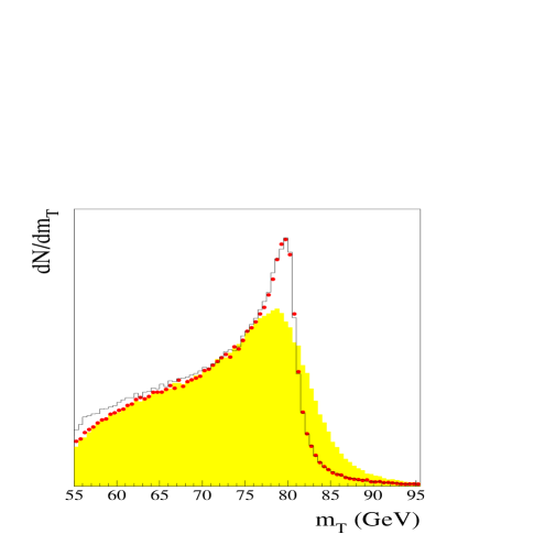
FIG. 3.: The $m_{T}$ spectrum for $W$ bosons with $q_{T}=0$ (——), with the correct $q_{T}$ distribution ($\bullet$), and with detector resolutions (shaded).

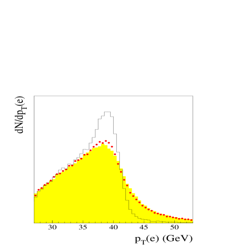
FIG. 4.: The $p_{T}(e)$ spectrum for $W$ bosons with $q_{T}=0$ (——), with the correct $q_{T}$ distribution ($\bullet$), and with detector resolutions (shaded).

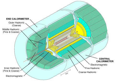
FIG. 5.: A cutaway view of the DØ calorimeter and tracking system.

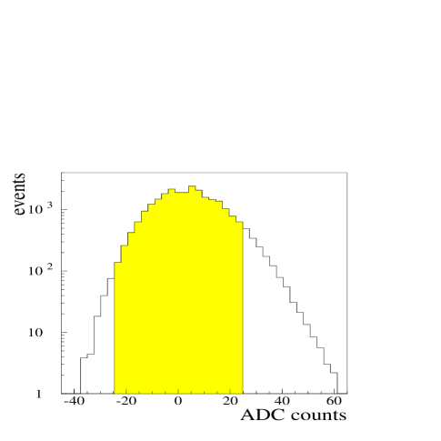
FIG. 6.: The pedestal spectrum of a central calorimeter cell, where the mean pedestal has been subtracted. The shaded region are the events removed by the zero-suppression.

FIG. 7.: The response of the liquid argon in the central calorimeter as monitored by $\alpha$ and $\beta$ sources.

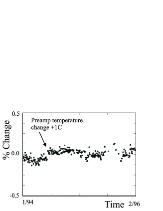
FIG. 8.: The percentage change in the central calorimeter gains over the course of the run.

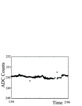
FIG. 9.: The change in the central calorimeter pedestals over the course of the run.

FIG. 10.: The fractional deviation of the reconstructed electron energy from the beam momentum from beam tests of a CC-EM module.

FIG. 11.: The fractional electron energy resolution measured in beam tests of a CC-EM module for the data ($\bullet$) and the parameterization (—–).

FIG. 12.: The relative efficiency of the Level 2 electron filter for a threshold of 20 GeV. The arrow indicates the cut applied in the final event selection.

FIG. 13.: The efficiency of a 15 GeV Level 2 $\hbox to0.0pt{\kern 1.00006pt/\hss}p_{T}$ requirement. The arrow indicates the cut applied in the final event selection.

FIG. 14.: Illustration of momentum vectors in the transverse plane for $Z\to ee$ candidates. The vectors drawn with thick lines are directly measured.

FIG. 15.: Illustration of momentum vectors in the transverse plane for $W\to e\nu$  candidates. The vectors drawn with thick lines are directly measured.

FIG. 16.: Distributions of the electron identification variables. The arrows indicate the cut values.

FIG. 17.: The luminosity distribution of the $W$ (——) and the $Z$ ($\bullet$) samples.

FIG. 18.: Polarization of the $W$ produced in $p\overline{p}$ collisions if the quark comes from the proton (left) and if the antiquark comes from the proton (right). The thick arrows indicate the orientation of the particle spins.

FIG. 19.: The calculations of $\alpha_{1}$(—–) and $\alpha_{2}$(- - -) as a function of the transverse momentum of the $W$ boson.

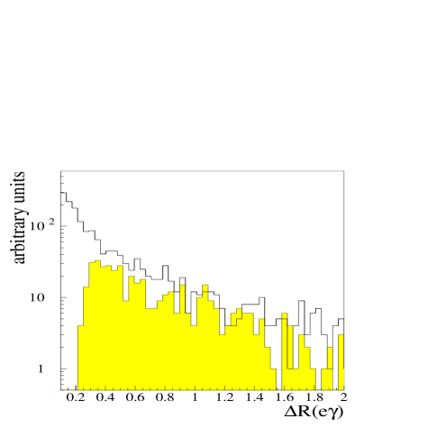
FIG. 20.: The distribution of $\Delta R(e\gamma)$ of photons from $W\to e\nu\gamma$ decays that are reconstructed as separate objects (shaded) and those that are not, either because they are too close to the electron or too low in energy (——).

FIG. 21.: The distribution of $z_{\rm vtx}(e_{1})-z_{\rm vtx}(e_{2})$ for the $Z\to ee$ sample ($\bullet$) and the fast Monte Carlo simulation (——).

FIG. 22.: The transverse energy flow into 1$\times$5 tower segments as a function of azimuthal separation from the electron in the $W$ sample.

FIG. 23.: The distribution of $\Delta u_{\parallel}$ in the $W$ signal sample.

FIG. 24.: The luminosity dependence of $\langle\Delta u_{\parallel}\rangle$.

FIG. 25.: The variation of $\langle\Delta u_{\parallel}\rangle$ as a function of $u_{\parallel}$. The region between the arrows is populated by the $W$ sample.

FIG. 26.: The transverse energy flow into 1$\times$5 tower segments as a function of the azimuthal separation from the electron for the electrons from $W\to e\nu$ decays ($\bullet$) and the superimposed Monte Carlo electron sample (——).

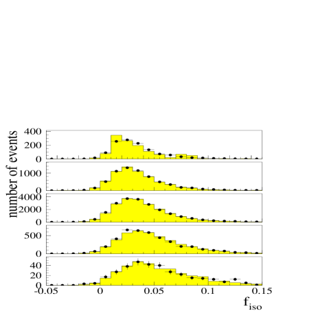
FIG. 27.: The isolation spectrum for five different $u_{\parallel}$ regions, $u_{\parallel}<-15$, $-15<u_{\parallel}<-5$, $-5<u_{\parallel}<5$, $5<u_{\parallel}<15$, $u_{\parallel}>15$ GeV (from top to bottom), for the electrons from $W\to e\nu$ decays ($\bullet$) and the superimposed electron sample (shaded).

FIG. 28.: The mean isolation versus $u_{\parallel}$ for the $W$ electron sample ($\circ$) and the superimposed Monte Carlo electron sample ($\bullet$).

FIG. 29.: The electron selection efficiency as a function of $u_{\parallel}$.

FIG. 30.: The background-subtracted $m_{\rm sym}$ distribution. The superimposed curve shows the Monte Carlo simulation.

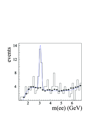
FIG. 31.: The dielectron invariant mass spectrum for the $J/\psi\to ee$ sample (histogram) and the background sample ($\bullet$). The smooth curve is a fit to the data.

FIG. 32.: The dielectron mass spectrum for the background data sample to the CC/CC $Z$ sample. The fit is an exponential.

FIG. 33.: The distribution of $m(ee)$ versus $f_{Z}$ for the CC-CC $Z\to ee$ sample.

FIG. 34.: The 68% confidence level contours in $\alpha_{\rm EM}$ and $\delta_{\rm EM}$ from the $J/\psi$, $\pi^{0}$, and $Z$ data. The inset shows an expanded view of the region where the $\chi^{2}$ is minimized.

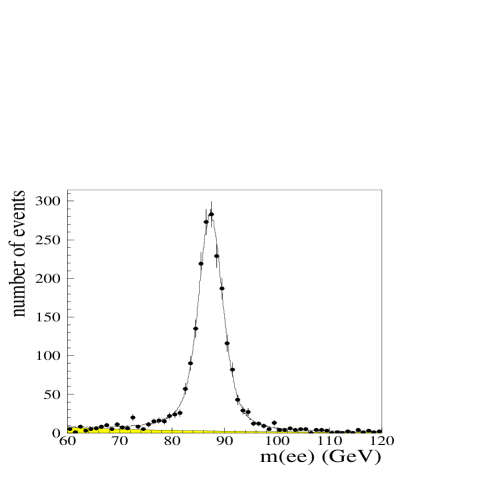
FIG. 35.: The dielectron mass spectrum from the CC-CC $Z$ sample. The superimposed curve shows the maximum likelihood fit and the shaded region the fitted background.

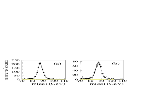
FIG. 36.: The dielectron mass spectra from (a) the tight/tight and (b) the tight/loose CC-CC $Z$ samples. The curves show the fitted Monte Carlo spectra.

FIG. 37.: The dielectron mass resolution versus the constant term $c_{\rm EM}$.

FIG. 38.: The recoil momentum response in the Monte Carlo $Z$ sample as a function of $q_{T}$.

FIG. 39.: The average $p_{\eta}(ee)+u_{\eta}$ versus $p_{\eta}(ee)$ for the $Z$ data ($\bullet$) and the fast Monte Carlo simulation ($\circ$) .

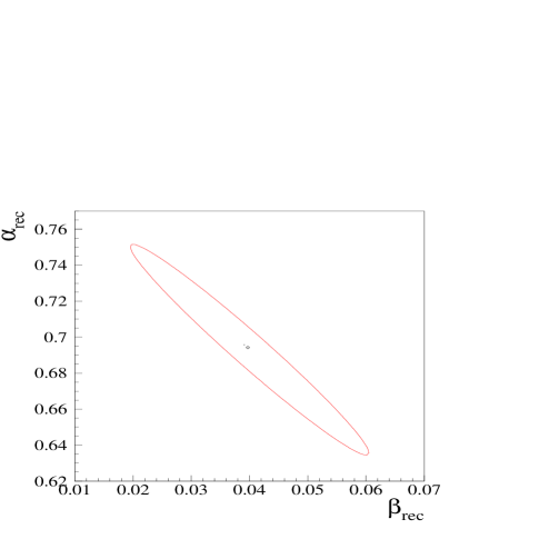
FIG. 40.: The $\chi^{2}_{0}+1$ contour for the recoil momentum response parameters.

FIG. 41.: The width of the $\eta$-balance distribution versus $p_{\eta}(ee)$ for the $Z$ data ($\bullet$) and the fast Monte Carlo simulation ($\circ$).

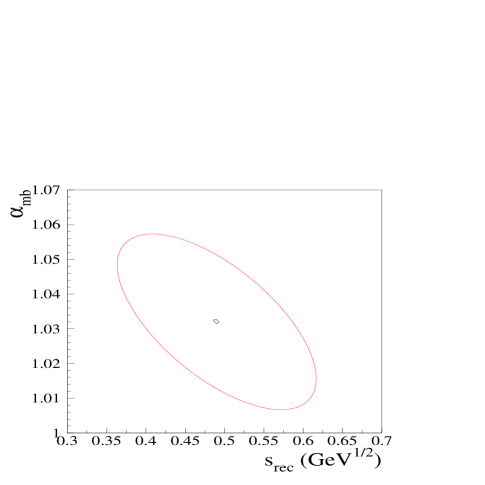
FIG. 42.: The $\chi_{0}^{2}+1$ contour for the recoil resolution parameters $\alpha_{\rm mb}$ and $s_{\rm rec}$.

FIG. 43.: The $\eta$-balance distribution for the $Z$ data ($\bullet$) and the fast Monte Carlo simulation (—–).

FIG. 44.: The $\xi$-balance distribution for the $Z$ data ($\bullet$) and the fast Monte Carlo simulation (—–).

FIG. 45.: The transverse energy flow in the $W$ ($\bullet$) and $Z$ (—–) data.

FIG. 46.: The resolution for transverse momentum balance, $\sigma_{T}$, versus the transverse energy flow, $S_{T}$, for minimum bias events ($\bullet$). The smooth curve is a fit (Eq. 52).

FIG. 47.: The $u_{\parallel}$ spectrum for the $W$ data ($\bullet$) and the Monte Carlo simulation (—–).

FIG. 48.: The $u_{\perp}$ spectrum for the $W$ data ($\bullet$) and the Monte Carlo simulation (—–).

FIG. 49.: The recoil momentum ($u_{T}$) spectrum for the $W$ data ($\bullet$) and the Monte Carlo simulation (—–). The arrow shows the location of the cut.

FIG. 50.: The azimuthal difference between electron and recoil directions for the $W$ data ($\bullet$) and the Monte Carlo simulation (—–).

FIG. 51.: Comparison of the $p_{T}(ee)$ data ($\bullet$) and simulation (—–) for the best fit $g_{2}$ using MRSA^′ parton distribution functions.

FIG. 52.: The background parameterizations for the $p_{T}(ee)$ spectrum.

FIG. 53.: The predicted $p_{T}(ee)$ spectra after detector simulation using MRSA^′ parton distribution functions and $g_{2}=0.18$, 0.58, and 0.98 GeV².

FIG. 54.: The $\hbox to0.0pt{\kern 1.00006pt/\hss}p_{T}$ spectra of a sample of events passing electron identification cuts (——) and a sample of events failing the cuts ($\bullet$).

FIG. 55.: The fraction of hadron background as a function of luminosity.

FIG. 56.: Shape of $m_{T}$, $p_{T}(e)$, and $p_{T}(\nu)$ spectra from hadron (——), $Z$ (- - -), and $\tau\to$hadron backgrounds ($\cdot\cdot\cdot\cdot\cdot$) with the proper relative normalization.

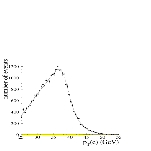
FIG. 57.: Spectrum of $p_{T}(e)$ from the $W$ data. The superimposed curve shows the maximum likelihood fit and the shaded region the estimated background.

FIG. 58.: The $\chi$ distribution for the fit to the $p_{T}(e)$ spectrum.

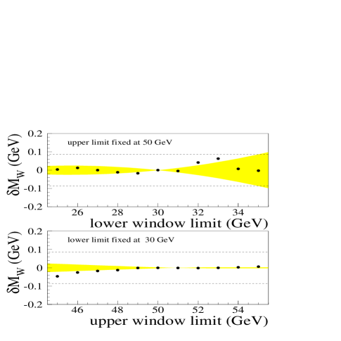
FIG. 59.: Variation of the fitted mass with the $p_{T}(e)$ fit window limits. See text for details.

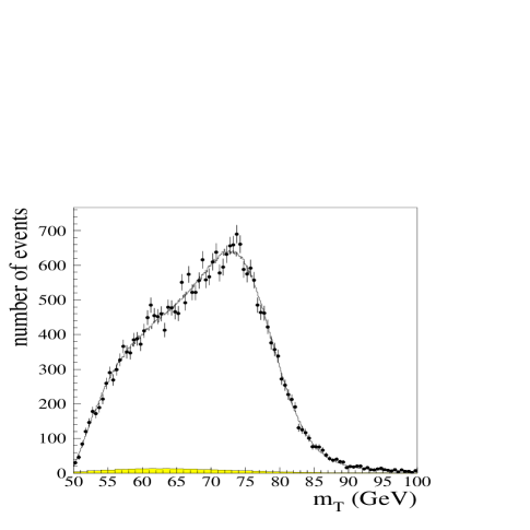
FIG. 60.: Spectrum of $m_{T}$ from the $W$ data. The superimposed curve shows the maximum likelihood fit and the shaded region shows the estimated background.

FIG. 61.: The likelihood function for the $m_{T}$ fit.

FIG. 62.: The $\chi$ distribution for the fit to the $m_{T}$ spectrum.

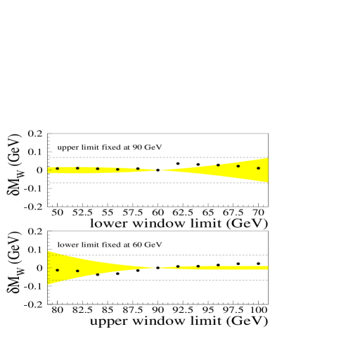
FIG. 63.: Variation of the fitted mass with the $m_{T}$ fit window limits. See text for details.

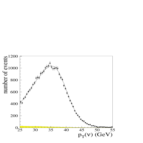
FIG. 64.: Spectrum of $p_{T}(\nu)$ from the $W$ data. The superimposed curve shows the maximum likelihood fit and the shaded region shows the estimated background.

FIG. 65.: The $\chi$ distribution for the fit to the $p_{T}(\nu)$ spectrum.

FIG. 66.: The fitted $W$ boson masses (a) in bins of luminosity from the $m_{T}$ ($\bullet$), $p_{T}(e)$ ($\circ$), and $p_{T}(\nu)$ ($\ast$) fits (the points are offset for clarity) and the fitted $Z$ boson masses (b). The solid line is the central value for the $m_{T}$ and $m(ee)$ mass fits respectively over the entire luminosity range and the dashed lines are the statistical errors.

FIG. 67.: Spectra of $m_{T}$ from $W$ data with $u_{\parallel}<0$ ($\circ$) and $u_{\parallel}>0$ ($\bullet$) compared to Monte Carlo simulations (——).

FIG. 68.: Spectra of $p_{T}(e)$ from $W$ data with $u_{\parallel}<0$ ($\circ$) and $u_{\parallel}>0$ ($\bullet$) compared to Monte Carlo simulations (——).

FIG. 69.: Spectra of $p_{T}(\nu)$ from $W$ data with $u_{\parallel}<0$ ($\circ$) and $u_{\parallel}>0$ ($\bullet$) compared to Monte Carlo simulations (——).

FIG. 70.: The variation in the $W$ mass from the $m_{T}$ fit as a function of $\phi(R)$.

FIG. 71.: The variation in the $W$ mass from the $m_{T}$ fit as a function of $\phi(e)$.

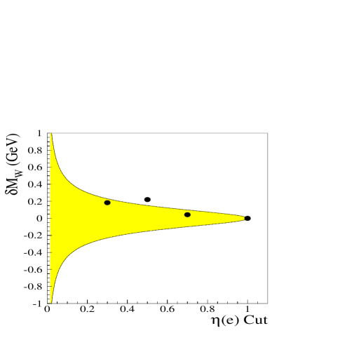
FIG. 72.: The variation in the $W$ mass versus the $\eta(e)$ cut. The shaded region is the expected statistical variation.

FIG. 73.: Value of $g_{2}$ as a function of $\Lambda_{\rm QCD}$. The error bar indicates the uncertainty in $g_{2}$ for fixed $\Lambda_{\rm QCD}$.

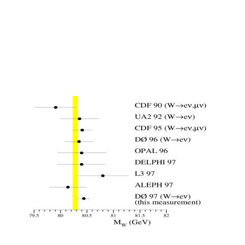
FIG. 74.: A comparison of this measurement with previously published $W$ mass measurements (Table XV). The shaded region indicates the predicted $W$ mass value from global fits to the $Z$ lineshape data [9].

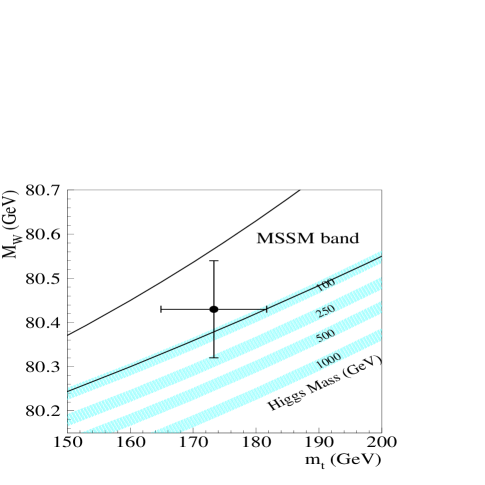
FIG. 75.: A comparison of the $W$ and top quark mass measurements by the DØ collaboration with the Standard Model predictions for different Higgs boson masses [53]. The width of the bands for each Higgs boson mass value indicates the uncertainty due to the error in $\alpha(M_{Z}^{2})$. Also shown is the range allowed by the MSSM [21].

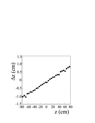
FIG. 76.: The difference between the predicted and the actual $z$-positions of the track center of gravity.

FIG. 77.: The $\chi^{2}$ versus $\alpha_{\rm CDC}$ value. The arrows indicate the statistical error on the fit.

TABLE I.: Electron selection criteria.

variable	CC (loose)	CC (tight)	EC (tight)
fiducial cuts	$|\Delta\phi|>0.02$	$|\Delta\phi|>0.02$	—
	$|z_{\rm cal}|<108$ cm	$|z_{\rm cal}|<108$ cm	$15\leq|i_{\eta}|\leq 25$
	—	$|z_{\rm trk}|<80$ cm	—
shower shape	$\chi^{2}<100$	$\chi^{2}<100$	$\chi^{2}<100$
isolation	$f_{\rm iso}<0.15$	$f_{\rm iso}<0.15$	$f_{\rm iso}<0.15$
track match	—	$\sigma_{\rm trk}<5$	$\sigma_{\rm trk}<10$

TABLE II.: Number of $W$ and $Z$ candidate events.

channel	$Z\to ee$			$W\to e\nu$
fiducial region of electrons	CC/CC	CC/CC	CC/EC	CC
$e$ quality (t=tight, l=loose)	t/l	t/t	t/t	t
pass Main Ring Veto	537	1225	1116	28323
fail Main Ring Veto	107	310	268	—

TABLE III.: Parton luminosity slope $\beta$ and fraction of sea-sea interactions $f_{\rm ss}$ in the $W$ and $Z$ production model. The $\beta$ value is given for $W\to e\nu$ decays with the electron in CC and for $Z\to ee$ decays with both electrons in CC.

	$Z$ production	$W$ production
	$\beta$ (GeV-1)	$\beta$ (GeV-1)	$f_{\rm ss}$
MRSA′ [35]	$3.6\times 10^{-3}$	$8.6\times 10^{-3}$	0.207
CTEQ3M [42]	$3.3\times 10^{-3}$	$8.7\times 10^{-3}$	0.203
CTEQ2M [43]	—	$8.8\times 10^{-3}$	0.203
MRSD$-^{\prime}$ [44]	$3.8\times 10^{-3}$	$9.6\times 10^{-3}$	0.201

TABLE IV.: $\Delta u_{\parallel}$ for the $W$ and $Z$ event samples.

Event Sample	$\sum E_{1\times 5}/\cosh\eta(e)$ (MeV)	$\Delta u_{\parallel}$ (MeV)
$W$	95.8$\pm$0.4	479$\pm$2$\pm$6
$Z$	93.6$\pm$1.3	468$\pm$7$\pm$6

TABLE V.: Fitted values of $g_{2}$ for different parton distribution functions. Uncertainties are statistical only.

	$p_{T}(ee)<15$ GeV	$\Delta\phi(ee)$
MRSA′	0.59$\pm$0.10 GeV2	0.64$\pm$0.14 GeV2
MRSD$-^{\prime}$	0.61$\pm$0.10 GeV2	0.70$\pm$0.15 GeV2
CTEQ3M	0.54$\pm$0.10 GeV2	0.57$\pm$0.13 GeV2
CTEQ2M	0.61$\pm$0.10 GeV2	0.67$\pm$0.14 GeV2

TABLE VI.: The results of the Monte Carlo ensemble tests fitting the $M_{W}$ mass for 105 samples of 28,323 events.

	mean	rms	correlation matrix
			$m_{T}$	$p_{T}(e)$	$p_{T}(\nu)$
	(GeV)	(GeV)
$m_{T}$	80.404	0.067	1	0.669	0.630
$p_{T}(e)$	80.415	0.091	0.669	1	0.180
$p_{T}(\nu)$	80.389	0.105	0.630	0.180	1

TABLE VII.: The confidence levels from Kolmogorov- Smirnov tests comparing collider data to Monte Carlo predictions for $M_{W}$=80.44 GeV.

	$m_{T}$	$p_{T}(e)$	$p_{T}(\nu)$
interval	60–90 GeV	30–50 GeV	30–50 GeV
$u_{T}<15$ GeV	0.25	0.81	0.20
$u_{\parallel}<0$	0.19	0.78	0.25
$u_{\parallel}>0$	0.61	0.80	0.48
$u_{T}<30$ GeV	0.55	0.99	0.58
interval	50–100 GeV	25–55 GeV	25–55 GeV
$u_{T}<15$ GeV	0.84	0.83	0.69
$u_{\parallel}<0$	0.77	0.67	0.62
$u_{\parallel}>0$	0.60	0.66	0.73
$u_{T}<30$ GeV	0.92	0.80	0.28

TABLE VIII.: Uncertainties in the $W$ mass measurement due to finite sample sizes.

	$m_{T}$ fit	$p_{T}(e)$ fit	$p_{T}(\nu)$ fit
$W$ sample	70 MeV	85 MeV	105 MeV
$Z$ sample	65 MeV	65 MeV	65 MeV
total	95 MeV	105 MeV	125 MeV

TABLE IX.: Uncertainties in the $W$ mass measurement due to $W$ production and decay model.

	$m_{T}$ fit	$p_{T}(e)$ fit	$p_{T}(\nu)$ fit
$p_{T}(W)$ spectrum	10 MeV	50 MeV	25 MeV
parton distribution functions	20 MeV	50 MeV	30 MeV
parton luminosity $\beta$	10 MeV	10 MeV	10 MeV
radiative decays	15 MeV	15 MeV	15 MeV
$W$ width	10 MeV	10 MeV	10 MeV
total	30 MeV	75 MeV	45 MeV

TABLE X.: Variation of fitted $W$ mass with choice of parton distribution function.

	$m_{T}$ fit	$p_{T}(e)$ fit	$p_{T}(\nu)$ fit
MRSA′	0	0	0
MRSD$-^{\prime}$	$20$ MeV	$19$ MeV	$20$ MeV
CTEQ3M	$5$ MeV	$48$ MeV	$22$ MeV
CTEQ2M	$-21$ MeV	$-17$ MeV	$-30$ MeV

TABLE XI.: Changes in fitted $W$ and $Z$ masses if radiative effects are varied.

variation	$m_{T}$ fit	$p_{T}(e)$ fit	$p_{T}(\nu)$ fit	$m(ee)$ fit
no radiative effects	50 MeV	43 MeV	30 MeV	143 MeV
vary $R_{0}$ by$\pm 0.1$	3 MeV	4 MeV	0 MeV	19 MeV

TABLE XII.: Uncertainties in the $W$ mass measurement due to detector model parameters.

	$m_{T}$ fit	$p_{T}(e)$ fit	$p_{T}(\nu)$ fit
calorimeter linearity	20 MeV	20 MeV	20 MeV
calorimeter uniformity	10 MeV	10 MeV	10 MeV
electron resolution	25 MeV	15 MeV	30 MeV
electron angle calibration	30 MeV	30 MeV	30 MeV
electron removal	15 MeV	15 MeV	20 MeV
selection bias	5 MeV	10 MeV	20 MeV
recoil resolution	25 MeV	10 MeV	90 MeV
recoil response	20 MeV	15 MeV	45 MeV
total	60 MeV	50 MeV	115 MeV

TABLE XIII.: Uncertainties in the $W$ mass measurement due to backgrounds.

	$m_{T}$ fit	$p_{T}(e)$ fit	$p_{T}(\nu)$ fit
hadrons	10 MeV	15 MeV	20 MeV
$Z\to ee$	5 MeV	10 MeV	5 MeV
$W\to\tau\nu$	negligible
cosmic rays	negligible
total	10 MeV	20 MeV	20 MeV

TABLE XIV.: Summary of results from the 1992–1993 and 1994–1995 data sets with the common and uncorrelated errors.

	1992–1993	1994–1995	common
$M_{W}$ from $m_{T}$ fit	80.35 GeV	80.44 GeV
$W$ statistics	140 MeV	70 MeV
$Z$ statistics	160 MeV	65 MeV
calorimeter linearity			20 MeV
calorimeter uniformity			10 MeV
electron resolution	70 MeV	20 MeV
electron angle calibration			30 MeV
recoil resolution	90 MeV	25 MeV
recoil response	50 MeV	20 MeV
electron removal	35 MeV	15 MeV
selection bias	30 MeV	5 MeV
backgrounds	35 MeV	10 MeV
$W$ production/decay			30 MeV
total uncertainty	255 MeV	105 MeV	50 MeV

TABLE XV.: Previously published measurements of the $W$ boson mass.

measurement	$M_{W}$ (GeV)	reference
CDF 90	79.91$\pm$0.39	[52]
UA2 92	80.36$\pm$0.37	[10]
CDF 95	80.41$\pm$0.18	[11]
DØ 96	80.35$\pm$0.27	[12]
OPAL 96	$80.40^{+0.45}_{-0.42}$	[13]
DELPHI 97	80.40$\pm$0.45	[14]
L3 97	$80.80^{+0.48}_{-0.42}$	[15]
ALEPH 97	80.14$\pm$0.35	[16]

REFERENCES

- [1] Visitor from Universidad San Francisco de Quito, Quito, Ecuador.
- [2] Visitor from IHEP, Beijing, China.
-
[1]
I. Adam, Ph.D. thesis,
Columbia University, 1997 (unpublished), Nevis Report #294,
http://www-d0.fnal.gov/publications_talks/ thesis/adam/ian_thesis_all.ps. -
[2]
E. Flattum, Ph.D. thesis,
Michigan State University, 1996 (unpublished),
http://www-d0.fnal.gov/publications_talks/ thesis/flattum/eric_thesis.ps. - [3] B. Abbott et al. (DØ Collaboration), FERMILAB-Pub-97/423-E, submitted to Phys. Rev. Lett.
- [4] G. Arnison et al. (UA1 Collaboration), Phys. Lett. B 122, 103 (1983).
- [5] M. Banner et al. (UA2 Collaboration), Phys. Lett. B 122, 476 (1983).
- [6] G. Arnison et al. (UA1 Collaboration), Phys. Lett. B 126, 398 (1983);
- [7] P. Bagnaia et al. (UA2 Collaboration), Phys. Lett. B 129, 130 (1983).
- [8] S.L. Glashow, Nucl. Phys. 22, 579 (1961); S. Weinberg, Phys. Rev. Lett. 19, 1264 (1967); A. Salam, Proceedings of the 8th Nobel Symposium, ed. N. Svartholm (Almqvist and Wiksells, Stockholm 1968), p. 367.
- [9] The LEP collaborations, the LEP Electroweak Working Group and the SLD Heavy Flavour Group, CERN-PPE/96-183 (unpublished).
- [10] J. Alitti et al. (UA2 Collaboration), Phys. Lett. B 276, 354 (1992). The value quoted in Table XV uses from Eq. 3.
- [11] F. Abe et al. (CDF Collaboration), Phys. Rev. Lett. 75, 11 (1995) and Phys. Rev. D 52, 4784 (1995).
- [12] S. Abachi et al. (DØ Collaboration), Phys. Rev. Lett. 77, 3309 (1996); B. Abbott et al. (DØ Collaboration), FERMILAB-Pub-97/328-E, submitted to Phys. Rev. D.
- [13] K. Ackerstaff et al. (OPAL Collaboration), Phys. Lett. B 389, 416 (1996).
- [14] P. Abreu et al. (Delphi Collaboration), Phys. Lett. B 397, 158 (1997).
- [15] M. Acciarri et al. (L3 Collaboration), Phys. Lett. B 398, 223 (1997).
- [16] R. Barate et al. (ALEPH Collaboration), Phys. Lett. B 401, 347 (1997).
- [17] A. Sirlin, Phys. Rev. D 22, 971 (1980); W. Marciano and A. Sirlin, Phys. Rev. D 22, 2695 (1980) and erratum-ibid. D 31, 213 (1985).
- [18] R.M. Barnett et al., Phys. Rev. D 54, 1 (1996).
- [19] S. Eidelmann and F. Jegerlehner, Z. Phys. C 67, 585 (1995).
- [20] S. Abachi et al. (DØ Collaboration), Phys. Rev. Lett. 79, 1197 (1997) and references therein.
- [21] P. Chankowski et al., Nucl. Phys. B 417, 101 (1994); D. Garcia and J. Sola, Mod. Phys. Lett. A 9, 211 (1994); A. Dabelstein, W. Hollik and W. Mosle, Perspectives for Electroweak Interactions in Collisions, ed. by B. A. Kniehl (World Scientific, Singapore, 1995) p345; D. Pierce et al., Nucl. Phys. B 491, 3 (1997).
- [22] H.T. Edwards, Annual Review of Nuclear and Particle Science, ed. J.D. Jackson et al., Vol. 35, p. 605 (1985).
- [23] S. Abachi et al. (DØ Collaboration), Nucl. Instrum. Methods in Phys. Res. A 338, 185 (1994).
- [24] M. Abolins et al. (DØ Collaboration), Nucl. Instrum. Methods in Phys. Res. A 280, 36 (1989); S. Abachi et al. (DØ Collaboration), Nucl. Instrum. Methods in Phys. Res. A 324, 53 (1993); H. Aihara et al. (DØ Collaboration), Nucl. Instrum. Methods in Phys. Res. A 325, 393 (1993).
-
[25]
Q. Zhu, Ph.D. thesis,
New York University, 1994 (unpublished),
http://www-d0.fnal.gov/publications_talks/ thesis/zhu/thesis_1side.ps. -
[26]
T.C. Heuring, Ph.D. thesis,
State University of New York at Stony Brook, 1993 (unpublished),
http://www-d0.fnal.gov/publications_talks/ thesis/heuring/thesis2s.ps. - [27] J.W.T. McKinley, Ph.D. thesis, Michigan State University, 1996 (unpublished).
- [28] F. Carminati et al., geantUsers Guide, CERN Program Library W5013, 1991 (unpublished).
- [29] S. Abachi et al. (DØ Collaboration), Phys. Rev. D 52, 4877 (1995).
- [30] G.A. Ladinsky and C.P. Yuan, Phys. Rev. D 50, 4239 (1994).
- [31] P.B. Arnold and R.P. Kauffman, Nucl. Phys. B 349, 381 (1991).
- [32] P.B. Arnold and M.H. Reno, Nucl. Phys. B 319, 37 (1989) and erratum-ibid. B 330, 284 (1990).
- [33] J. Collins and D. Soper, Nucl. Phys. B 193, 381 (1981) and erratum-ibid. B 213, 545 (1983); J. Collins, D. Soper, and G. Sterman, Nucl. Phys. B 250, 199 (1985).
- [34] G. Altarelli et al., Nucl. Phys. B 246, 12 (1984).
- [35] A.D. Martin, W.J. Stirling, and R.G. Roberts, Phys. Rev. D 50, 6734 (1994) and Phys. Rev. D 51, 4756 (1995).
- [36] S. Abachi et al. (DØ Collaboration), Phys. Rev. Lett. 75, 1456 (1995).
- [37] G. Marchesini et al., Comput. Phys. Commun. 67 465 (1992), release 5.7.
- [38] H. Plotow-Besch, CERN-PPE W5051 (1997), release 7.02.
- [39] E. Mirkes, Nucl. Phys. B 387, 3 (1992).
- [40] J. Collins and D. Soper, Phys. Rev. D 16, 2219 (1977).
- [41] F.A. Berends and R. Kleiss, Z. Phys. C 27, 365 (1985); F.A. Berends et al., Z. Phys. C 27, 155 (1985).
- [42] H.L. Lai et al., Phys. Rev. D 51, 4763 (1995).
- [43] J. Botts et al., Phys. Lett. B 304, 159 (1993).
- [44] A.D. Martin, W.J. Stirling, and R.G. Roberts, Phys. Lett. B 306, 145 (1993) and erratum-ibid. B 309, 492 (1993).
-
[45]
T. Taylor Thomas, Ph.D. thesis,
Northwestern University, 1997 (unpublished),
http://www-d0.fnal.gov/publications_talks/ thesis/thomas/thesis_2side.ps. - [46] This test returns a confidence level that is uniformly distributed between 0 and 1 if the two spectra derive from the same parent distribution. See e.g. A.G. Frodesen, O. Skjeggestad, and H. Tøfte, Probability and Statistics in Particle Physics, Columbia University Press (1979).
- [47] D. Casey, Ph.D. thesis, University of Rochester, 1997 (unpublished).
- [48] These unpublished fits were made available by the CTEQ collaboration.
- [49] S. Abachi et al. (DØ Collaboration), Phys. Rev. Lett. 79, 1203 (1997).
- [50] F. Abe et al. (CDF Collaboration), Phys. Rev. Lett. 74, 850 (1995).
- [51] U. Baur et al., Phys. Rev. D 56, 140 (1997); U. Baur et al., Proceedings of the 1996 DPF/DPB Summer Study on High Energy Physics, edited by D.G. Cassel, L. Trindle Gennari, R.H. Siemann (Stanford Linear Accelerator Center, 1997), Vol. 1, p. 514; U. Baur, S. Keller, and D. Wackeroth ibid., Vol. 1, p. 517; U. Baur, S. Keller, and W.K. Sakumoto, FERMILAB-Pub-97/221-T (to be published in Phys. Rev. D).
- [52] F. Abe et al. (CDF Collaboration), Phys. Rev. Lett. 65, 2243 (1990) and Phys. Rev. D 43, 2070 (1991).
- [53] G. Degrassi et al. CERN-TH-97-197, to be published in Phys. Lett.; G. Degrassi, P. Gambino, and A. Sirlin, Phys. Lett. B 394, 188 (1997).