Search for Lepton Flavor Violation
in $ep$ Collisions at 300 GeV
Center of Mass Energy

Using the ZEUS detector at the HERA electron-proton collider, we have searched for lepton flavor violation in $ep$ collisions at a center–of–mass energy ($\sqrt{s}$) of 300 GeV. Events of the type $e+p\to{\ell}+X$ with a final–state lepton of high transverse momentum, ${\ell}=\mu$ or $\tau$, were sought. No evidence was found for lepton flavor violation in the combined 1993 and 1994 data samples, for which the integrated luminosities were 0.84 $pb^{-1}$ for $e^{-}p$ collisions and 2.94 $pb^{-1}$ for $e^{+}p$ collisions. Limits on coupling vs. mass are provided for leptoquarks and $R$–parity violating squarks. For flavor violating couplings of electromagnetic strength, we set 95% confidence level lower limits on leptoquark masses between 207 GeV and 272 GeV, depending on the leptoquark species and final–state lepton. For leptoquark masses larger than 300 GeV, limits on flavor–changing couplings are determined, many of which supersede prior limits from rare decay processes.

DESY 96-161 ISSN 0418-9833

The ZEUS Collaboration

M. Derrick, D. Krakauer, S. Magill, D. Mikunas, B. Musgrave, J.R. Okrasiński, J. Repond, R. Stanek, R.L. Talaga, H. Zhang
Argonne National Laboratory, Argonne, IL, USA ^p

M.C.K. Mattingly
Andrews University, Berrien Springs, MI, USA

F. Anselmo, P. Antonioli, G. Bari, M. Basile, L. Bellagamba, D. Boscherini, A. Bruni, G. Bruni, P. Bruni, G. Cara Romeo, G. Castellini¹, L. Cifarelli², F. Cindolo, A. Contin, M. Corradi, I. Gialas, P. Giusti, G. Iacobucci, G. Laurenti, G. Levi, A. Margotti, T. Massam, R. Nania, F. Palmonari, A. Pesci, A. Polini, G. Sartorelli, Y. Zamora Garcia³, A. Zichichi
University and INFN Bologna, Bologna, Italy ^f

C. Amelung, A. Bornheim, J. Crittenden, R. Deffner, M. Eckert, L. Feld, A. Frey⁴, M. Geerts⁵, M. Grothe, H. Hartmann, K. Heinloth, L. Heinz, E. Hilger, H.-P. Jakob, U.F. Katz, S. Mengel⁶, E. Paul, M. Pfeiffer, Ch. Rembser, D. Schramm⁷, J. Stamm, R. Wedemeyer
Physikalisches Institut der Universität Bonn, Bonn, Germany ^c

S. Campbell-Robson, A. Cassidy, W.N. Cottingham, N. Dyce, B. Foster, S. George, M.E. Hayes, G.P. Heath, H.F. Heath, D. Piccioni, D.G. Roff, R.J. Tapper, R. Yoshida
H.H. Wills Physics Laboratory, University of Bristol, Bristol, U.K. ^o

M. Arneodo⁸, R. Ayad, M. Capua, A. Garfagnini, L. Iannotti, M. Schioppa, G. Susinno
Calabria University, Physics Dept.and INFN, Cosenza, Italy ^f

A. Caldwell⁹, N. Cartiglia, Z. Jing, W. Liu, J.A. Parsons, S. Ritz¹⁰, F. Sciulli, P.B. Straub, L. Wai¹¹, S. Yang¹², Q. Zhu
Columbia University, Nevis Labs., Irvington on Hudson, N.Y., USA ^q

P. Borzemski, J. Chwastowski, A. Eskreys, Z. Jakubowski, M.B. Przybycień, M. Zachara, L. Zawiejski
Inst. of Nuclear Physics, Cracow, Poland ^j

L. Adamczyk, B. Bednarek, K. Jeleń, D. Kisielewska, T. Kowalski, M. Przybycień, E. Rulikowska-Zarȩbska, L. Suszycki, J. Zaja̧c
Faculty of Physics and Nuclear Techniques, Academy of Mining and Metallurgy, Cracow, Poland ^j

Z. Duliński, A. Kotański
Jagellonian Univ., Dept. of Physics, Cracow, Poland ^k

G. Abbiendi¹³, L.A.T. Bauerdick, U. Behrens, H. Beier, J.K. Bienlein, G. Cases, O. Deppe, K. Desler, G. Drews, M. Flasiński¹⁴, D.J. Gilkinson, C. Glasman, P. Göttlicher, J. Große-Knetter, T. Haas, W. Hain, D. Hasell, H. Heßling, Y. Iga, K.F. Johnson¹⁵, P. Joos, M. Kasemann, R. Klanner, W. Koch, U. Kötz, H. Kowalski, J. Labs, A. Ladage, B. Löhr, M. Löwe, D. Lüke, J. Mainusch¹⁶, O. Mańczak, J. Milewski, T. Monteiro¹⁷, J.S.T. Ng, D. Notz, K. Ohrenberg, K. Piotrzkowski, M. Roco, M. Rohde, J. Roldán, U. Schneekloth, W. Schulz, F. Selonke, B. Surrow, E. Tassi, T. Voß, D. Westphal, G. Wolf, U. Wollmer, C. Youngman, W. Zeuner
Deutsches Elektronen-Synchrotron DESY, Hamburg, Germany

H.J. Grabosch, S.M. Mari¹⁸, A. Meyer, S. Schlenstedt
DESY-IfH Zeuthen, Zeuthen, Germany

G. Barbagli, E. Gallo, P. Pelfer
University and INFN, Florence, Italy ^f

G. Maccarrone, S. De Pasquale, L. Votano
INFN, Laboratori Nazionali di Frascati, Frascati, Italy ^f

A. Bamberger, S. Eisenhardt, T. Trefzger¹⁹, S. Wölfle
Fakultät für Physik der Universität Freiburg i.Br., Freiburg i.Br., Germany ^c

J.T. Bromley, N.H. Brook, P.J. Bussey, A.T. Doyle, D.H. Saxon, L.E. Sinclair, E. Strickland, M.L. Utley, R. Waugh, A.S. Wilson
Dept. of Physics and Astronomy, University of Glasgow, Glasgow, U.K. ^o

A. Dannemann²⁰, U. Holm, D. Horstmann, R. Sinkus²¹, K. Wick
Hamburg University, I. Institute of Exp. Physics, Hamburg, Germany ^c

B.D. Burow²², L. Hagge¹⁶, E. Lohrmann, G. Poelz, W. Schott, F. Zetsche
Hamburg University, II. Institute of Exp. Physics, Hamburg, Germany ^c

T.C. Bacon, N. Brümmer, I. Butterworth, V.L. Harris, G. Howell, B.H.Y. Hung, L. Lamberti²³, K.R. Long, D.B. Miller, N. Pavel, A. Prinias²⁴, J.K. Sedgbeer, D. Sideris, A.F. Whitfield
Imperial College London, High Energy Nuclear Physics Group, London, U.K. ^o

U. Mallik, M.Z. Wang, S.M. Wang, J.T. Wu
University of Iowa, Physics and Astronomy Dept., Iowa City, USA ^p

P. Cloth, D. Filges
Forschungszentrum Jülich, Institut für Kernphysik, Jülich, Germany

S.H. An, G.H. Cho, B.J. Ko, S.B. Lee, S.W. Nam, H.S. Park, S.K. Park
Korea University, Seoul, Korea ^h

S. Kartik, H.-J. Kim, R.R. McNeil, W. Metcalf, V.K. Nadendla
Louisiana State University, Dept. of Physics and Astronomy, Baton Rouge, LA, USA ^p

F. Barreiro, J.P. Fernandez, R. Graciani, J.M. Hernández, L. Hervás, L. Labarga, M. Martinez, J. del Peso, J. Puga, J. Terron, J.F. de Trocóniz
Univer. Autónoma Madrid, Depto de Física Teóríca, Madrid, Spain ⁿ

F. Corriveau, D.S. Hanna, J. Hartmann, L.W. Hung, J.N. Lim, C.G. Matthews²⁵, W.N. Murray, A. Ochs, P.M. Patel, M. Riveline, D.G. Stairs, M. St-Laurent, R. Ullmann, G. Zacek²⁵
McGill University, Dept. of Physics, Montréal, Québec, Canada ${}^{a},$  ^b

T. Tsurugai
Meiji Gakuin University, Faculty of General Education, Yokohama, Japan

V. Bashkirov, B.A. Dolgoshein, A. Stifutkin
Moscow Engineering Physics Institute, Mosocw, Russia ^l

G.L. Bashindzhagyan²⁶, P.F. Ermolov, L.K. Gladilin, Yu.A. Golubkov, V.D. Kobrin, I.A. Korzhavina, V.A. Kuzmin, O.Yu. Lukina, A.S. Proskuryakov, A.A. Savin, L.M. Shcheglova, A.N. Solomin, N.P. Zotov
Moscow State University, Institute of Nuclear Physics, Moscow, Russia ^m

M. Botje, F. Chlebana, J. Engelen, M. de Kamps, P. Kooijman, A. Kruse, A. van Sighem, H. Tiecke, W. Verkerke, J. Vossebeld, M. Vreeswijk, L. Wiggers, E. de Wolf, R. van Woudenberg²⁷
NIKHEF and University of Amsterdam, Netherlands ⁱ

D. Acosta, B. Bylsma, L.S. Durkin, J. Gilmore, C.M. Ginsburg, C.L. Kim, C. Li, T.Y. Ling, P. Nylander, I.H. Park, T.A. Romanowski²⁸
Ohio State University, Physics Department, Columbus, Ohio, USA ^p

D.S. Bailey, R.J. Cashmore²⁹, A.M. Cooper-Sarkar, R.C.E. Devenish, N. Harnew, M. Lancaster³⁰,
L. Lindemann, J.D. McFall, C. Nath, V.A. Noyes²⁴, A. Quadt, J.R. Tickner, H. Uijterwaal, R. Walczak, D.S. Waters, F.F. Wilson, T. Yip
Department of Physics, University of Oxford, Oxford, U.K. ^o

A. Bertolin, R. Brugnera, R. Carlin, F. Dal Corso, M. De Giorgi, U. Dosselli, S. Limentani, M. Morandin, M. Posocco, L. Stanco, R. Stroili, C. Voci, F. Zuin
Dipartimento di Fisica dell’ Universita and INFN, Padova, Italy ^f

J. Bulmahn, R.G. Feild³¹, B.Y. Oh, J.J. Whitmore
Pennsylvania State University, Dept. of Physics, University Park, PA, USA ^q

G. D’Agostini, G. Marini, A. Nigro
Dipartimento di Fisica, Univ. ’La Sapienza’ and INFN, Rome, Italy ${}^{f}~{}$

J.C. Hart, N.A. McCubbin, T.P. Shah
Rutherford Appleton Laboratory, Chilton, Didcot, Oxon, U.K. ^o

E. Barberis, T. Dubbs, C. Heusch, M. Van Hook, W. Lockman, J.T. Rahn, H.F.-W. Sadrozinski, A. Seiden, D.C. Williams
University of California, Santa Cruz, CA, USA ^p

J. Biltzinger, R.J. Seifert, O. Schwarzer, A.H. Walenta
Fachbereich Physik der Universität-Gesamthochschule Siegen, Germany ^c

H. Abramowicz, G. Briskin, S. Dagan³², T. Doeker³², A. Levy²⁶
Raymond and Beverly Sackler Faculty of Exact Sciences, School of Physics, Tel-Aviv University, Tel-Aviv, Israel ^e

J.I. Fleck³³, M. Inuzuka, T. Ishii, M. Kuze, S. Mine, M. Nakao, I. Suzuki, K. Tokushuku,
K. Umemori, S. Yamada, Y. Yamazaki
Institute for Nuclear Study, University of Tokyo, Tokyo, Japan ^g

M. Chiba, R. Hamatsu, T. Hirose, K. Homma, S. Kitamura³⁴, T. Matsushita, K. Yamauchi
Tokyo Metropolitan University, Dept. of Physics, Tokyo, Japan ^g

R. Cirio, M. Costa, M.I. Ferrero, S. Maselli, C. Peroni, R. Sacchi, A. Solano, A. Staiano
Universita di Torino, Dipartimento di Fisica Sperimentale and INFN, Torino, Italy ^f

M. Dardo
II Faculty of Sciences, Torino University and INFN - Alessandria, Italy ^f

D.C. Bailey, F. Benard, M. Brkic, C.-P. Fagerstroem, G.F. Hartner, K.K. Joo, G.M. Levman, J.F. Martin, R.S. Orr, S. Polenz, C.R. Sampson, D. Simmons, R.J. Teuscher
University of Toronto, Dept. of Physics, Toronto, Ont., Canada ^a

J.M. Butterworth, C.D. Catterall, T.W. Jones, P.B. Kaziewicz, J.B. Lane, R.L. Saunders, J. Shulman, M.R. Sutton
University College London, Physics and Astronomy Dept., London, U.K. ^o

B. Lu, L.W. Mo
Virginia Polytechnic Inst. and State University, Physics Dept., Blacksburg, VA, USA ^q

W. Bogusz, J. Ciborowski, J. Gajewski, G. Grzelak³⁵, M. Kasprzak, M. Krzyżanowski,
K. Muchorowski³⁶, R.J. Nowak, J.M. Pawlak, T. Tymieniecka, A.K. Wróblewski, J.A. Zakrzewski, A.F. Żarnecki
Warsaw University, Institute of Experimental Physics, Warsaw, Poland ^j

M. Adamus
Institute for Nuclear Studies, Warsaw, Poland ^j

C. Coldewey, Y. Eisenberg³², D. Hochman, U. Karshon³², D. Revel³², D. Zer-Zion
Weizmann Institute, Nuclear Physics Dept., Rehovot, Israel ^d

W.F. Badgett, J. Breitweg, D. Chapin, R. Cross, S. Dasu, C. Foudas, R.J. Loveless, S. Mattingly, D.D. Reeder, S. Silverstein, W.H. Smith, A. Vaiciulis, M. Wodarczyk
University of Wisconsin, Dept. of Physics, Madison, WI, USA ^p

S. Bhadra, M.L. Cardy³⁷, W.R. Frisken, M. Khakzad, W.B. Schmidke
York University, Dept. of Physics, North York, Ont., Canada ^a

¹ also at IROE Florence, Italy
² now at Univ. of Salerno and INFN Napoli, Italy
³ supported by Worldlab, Lausanne, Switzerland
⁴ now at Univ. of California, Santa Cruz
⁵ now a self-employed consultant
⁶ now at VDI-Technologiezentrum Düsseldorf
⁷ now at Commasoft, Bonn
⁸ also at University of Torino and Alexander von Humboldt Fellow
⁹ Alexander von Humboldt Fellow
¹⁰ Alfred P. Sloan Foundation Fellow
¹¹ now at University of Washington, Seattle
¹² now at California Institute of Technology, Los Angeles
¹³ supported by an EC fellowship number ERBFMBICT 950172
¹⁴ now at Inst. of Computer Science, Jagellonian Univ., Cracow
¹⁵ visitor from Florida State University
¹⁶ now at DESY Computer Center
¹⁷ supported by European Community Program PRAXIS XXI
¹⁸ present address: Dipartimento di Fisica, Univ. “La Sapienza”, Rome
¹⁹ now at ATLAS Collaboration, Univ. of Munich
²⁰ now at Star Division Entwicklungs- und Vertriebs-GmbH, Hamburg
²¹ now at Philips Medizin Systeme, Hamburg
²² also supported by NSERC, Canada
²³ supported by an EC fellowship
²⁴ PPARC Post-doctoral Fellow
²⁵ now at Park Medical Systems Inc., Lachine, Canada
²⁶ partially supported by DESY
²⁷ now at Philips Natlab, Eindhoven, NL
²⁸ now at Department of Energy, Washington
²⁹ also at University of Hamburg, Alexander von Humboldt Research Award
³⁰ now at Lawrence Berkeley Laboratory, Berkeley
³¹ now at Yale University, New Haven, CT
³² supported by a MINERVA Fellowship
³³ supported by the Japan Society for the Promotion of Science (JSPS)
³⁴ present address: Tokyo Metropolitan College of Allied Medical Sciences, Tokyo 116, Japan
³⁵ supported by the Polish State Committee for Scientific Research, grant No. 2P03B09308
³⁶ supported by the Polish State Committee for Scientific Research, grant No. 2P03B09208
³⁷ now at TECMAR Incorporated, Toronto

a	supported by the Natural Sciences and Engineering Research Council of Canada (NSERC)
b	supported by the FCAR of Québec, Canada
c	supported by the German Federal Ministry for Education and Science, Research and Technology (BMBF), under contract numbers 057BN19P, 057FR19P, 057HH19P, 057HH29P, 057SI75I
d	supported by the MINERVA Gesellschaft für Forschung GmbH, the Israel Academy of Science and the U.S.-Israel Binational Science Foundation
e	supported by the German Israeli Foundation, and by the Israel Academy of Science
f	supported by the Italian National Institute for Nuclear Physics (INFN)
g	supported by the Japanese Ministry of Education, Science and Culture (the Monbusho) and its grants for Scientific Research
h	supported by the Korean Ministry of Education and Korea Science and Engineering Foundation
i	supported by the Netherlands Foundation for Research on Matter (FOM)
j	supported by the Polish State Committee for Scientific Research, grants No. 115/E-343/SPUB/P03/109/95, 2P03B 244 08p02, p03, p04 and p05, and the Foundation for Polish-German Collaboration (proj. No. 506/92)
k	supported by the Polish State Committee for Scientific Research (grant No. 2 P03B 083 08) and Foundation for Polish-German Collaboration
l	partially supported by the German Federal Ministry for Education and Science, Research and Technology (BMBF)
m	supported by the German Federal Ministry for Education and Science, Research and Technology (BMBF), and the Fund of Fundamental Research of Russian Ministry of Science and Education and by INTAS-Grant No. 93-63
n	supported by the Spanish Ministry of Education and Science through funds provided by CICYT
o	supported by the Particle Physics and Astronomy Research Council
p	supported by the US Department of Energy
q	supported by the US National Science Foundation

1 Introduction

Lepton flavor is conserved in all interactions of the Standard Model (SM); discovery of lepton–flavor violation (LFV) in any form would be evidence for physics beyond our principal particle physics paradigm. Many searches for specific reactions which violate lepton flavor have been performed. The most sensitive include searches for $\mu+N\to e+N$ using very low–energy muons[1], for the forbidden muon decay $\mu\to e\gamma$ [2], and for forbidden leptonic kaon decays[3]. The limits from these processes are sensitive to $e\leftrightarrow\mu$ flavor change, but not to $e\leftrightarrow\tau$. Also, each of these processes involves specific quark flavors: in the first case, only first generation quarks participate; in the second case, for mechanisms which involve virtual quarks, the same quark flavor must couple to both $e$ and $\mu$; in the last case, strange quarks must be involved. Since lepton flavor change could involve the $\tau$-lepton or could be accompanied by quark flavor change, there may be LFV reactions which would be invisible to these very sensitive experiments. Hence, we have no a priori reason to assume that flavor violation, should it exist, will be visible through these specific reactions. Therefore, though less sensitive in an absolute sense, other manifestations of flavor violation, like forbidden leptonic decays of $B$– and $D$–mesons and of $\tau$–leptons, are being investigated [4].

We report here a search for LFV carried out by the ZEUS collaboration at the HERA $ep$ collider where we have sought instances of the reaction

$$e+p\rightarrow{\ell}+X,$$ (1)

where ${\ell}$ represents an isolated final–state $\mu$ or $\tau$ with large transverse momentum and $X$ represents the hadronic final state. Processes with such topologies can be found in ZEUS with good efficiency and with little background. It should be emphasized that any reaction of the type (1) in which a final–state high–energy $\mu$ or $\tau$ replaces the incident electron would be direct evidence for physics beyond the Standard Model, independent of the underlying mechanism. Furthermore, this reaction should occur at some level for a wide range of possible LFV mechanisms. LFV mechanisms which also involve a quark flavor change, or which are stronger for heavier quarks [5] may be seen more readily at HERA, where the sensitivity is largely independent of quark flavor, than in low–energy experiments.

The lepton–flavor violating reaction (1) could occur via $s$–, $u$–, or $t$–channel exchanges as shown in figure  1. For the $s$– and $u$–channel processes the exchanged particle has the quantum numbers of a leptoquark (or an $R$–parity violating squark). The cross sections depend on the leptoquark species and mass, and on the couplings, $\lambda_{eq_{1}}$ and $\lambda_{{\ell}q_{2}}$ shown in figure 1. For the case of $t$–channel exchange, the process would be mediated by a flavor–changing neutral boson.

For definiteness, we will describe reaction (1) with leptoquarks as the carrier of the LFV force, treating separately the cases of direct leptoquark production and the virtual effects of leptoquarks with masses above 300 GeV. The similarity of production formulae between $R$–parity–violating squarks and certain leptoquarks permits us to relate the couplings implied by the two mechanisms for a specified cross section. Results on flavor violation induced by leptogluons or by flavor–changing neutral bosons as well as details of the technique used in this analysis are also available [6]. The H1 collaboration [7] has also searched for direct production of leptoquarks with flavor–violating couplings using similar methods.

This analysis is based on an integrated luminosity of 0.84 $pb^{-1}$ (2.94 $pb^{-1}$ ) of $e^{-}p$ ($e^{+}p$) data taken during the 1993 and 1994 running periods. Beam energies at HERA were 26.7 GeV (27.5 GeV) for the electron beam in 1993 (1994) and 820 GeV for the proton beam. The resulting center–of–mass energy of 296 GeV (300 GeV) is an order of magnitude higher than for fixed–target lepton–nucleon scattering experiments.

2 Scenarios of Lepton Flavor Violation

2.1 Leptoquarks

A leptoquark (LQ) is a hypothetical color triplet boson with fractional electric charge, and non–zero lepton and baryon numbers. Such particles are often invoked in extensions of the SM, e.g. in grand unified theories and technicolor models [8]. It is possible, indeed desirable in some models, that a LQ couple to multiple lepton and/or quark flavors, thereby providing a mechanism for flavor violation.

The simplest models involving a flavor–violating leptoquark would be characterized by three parameters: the leptoquark mass, and the coupling at each lepton–quark–leptoquark vertex. In order to avoid models which would involve additional parameters, we have assumed the following four points:

1. the LQ has ${\mbox{\rm SU}}(3)_{C}\times{\mbox{\rm SU}}(2)_{L}\times{\mbox{\rm U}}(1)_{Y}$ invariant couplings,

2. the LQ has either left– or right–handed couplings, but not both (i.e. $\lambda_{L}\lambda_{R}=0$),

3. the members of each weak–isospin multiplet are degenerate in mass,

4. one LQ species dominates the production process.

There are fourteen species of leptoquarks which satisfy these conditions [9]. For fermion number $F\equiv L+3B$ ($L$ and $B$ denote lepton and baryon number) equal to zero, the species are denoted [8] $S_{1/2}^{L}$, $S_{1/2}^{R}$, ${\tilde{S}}_{1/2}^{L}$, $V_{0}^{L}$, $V_{0}^{R}$, ${\tilde{V}}_{0}^{R}$, and $V_{1}^{L}$. For $F=2$, they are $S_{0}^{L}$, $S_{0}^{R}$, ${\tilde{S}}_{0}^{R}$, $S_{1}^{L}$, $V_{1/2}^{L}$, $V_{1/2}^{R}$, and ${\tilde{V}}_{1/2}^{L}$. Here $S$ and $V$ indicate scalar and vector leptoquarks respectively, which couple to left– ($L$) or right–handed ($R$) leptons as indicated by the superscript. The subscript gives the weak isospin of the LQ. In $s$-channel reactions, $F=0$ LQ cross sections are higher in $e^{+}p$ collisions, where they are produced via $e^{+}q$ fusion, than in $e^{-}p$ collisions where $e^{-}{\overline{q}}$ fusion occurs. The reverse is true for an $F=2$ leptoquark.

A LQ scenario is defined by the leptoquark species, by the generations of the quarks which couple to the electron and to the final–state lepton, and by the final–state lepton flavor. Hence there are $14\times 3\times 3\times 2=252$ different LQ scenarios, each characterized by two dimensionless couplings, $\lambda_{eq_{1}}$ and $\lambda_{{\ell}q_{2}}$, defined in figure 1, which could induce flavor violation. Such LQs would also mediate flavor–conserving interactions with a final–state $e$ or $\nu_{e}$, which are not considered in this paper.

As an illustration, we show in figure 2 the present limits [10] on $\lambda_{eq_{1}}\lambda_{{\ell}q_{2}}$ versus LQ mass, $M_{\scriptscriptstyle LQ}$, for reactions which could proceed through the left–handed scalar isosinglet LQ, $S_{0}^{L}$. Note that each of the limits assumes that specific quark flavors couple to $e$ and $\mu$. For example, the most sensitive limit, from $\mu N\to eN$, applies only for first–generation quarks in both initial and final states. Also in this figure are the results of direct searches for leptoquark pair production. Searches in $e^{+}e^{-}$ collisions at LEP[11] exclude scalar leptoquarks lighter than about 45 GeV which couple to $e$, $\mu$, $\tau$, or any neutrino. For leptoquarks with couplings of electromagnetic strength, masses below 73 GeV are excluded. While the LEP experiments did not search for flavor violation, their non-observation of $e{\overline{e}}q{\overline{q}}$, $\mu{\overline{\mu}}q{\overline{q}}$, $\tau{\overline{\tau}}q{\overline{q}}$, or $\nu{\overline{\nu}}q{\overline{q}}$ final states kinematically consistent with leptoquark pair production imply flavor–violating leptoquark mass limits which are weaker by at most a few GeV. At the Tevatron [12], searches in $p{\overline{p}}$ collisions have excluded scalar leptoquarks lighter than 131 GeV (96 GeV) for an assumed branching fraction to $q\mu$ of 100% (50%). These limits on $M_{\scriptscriptstyle LQ}$ are independent of the LQ couplings in most models.

The LQ–induced cross sections for reaction (1), given in detail in the appendix, depend on the initial quark density, the couplings, and the species of LQ involved in the reaction, as well as on the kinematic event variables $x$ (the Bjorken scaling variable) and $y$ (the inelasticity). Here $x$ is defined as $x=-q^{2}/(2q\cdot P)$ and $y$ as $y=(q\cdot P)/(k\cdot P)$, where $k$, $k^{\prime}$, and $P$ are the four–momenta of the initial–state electron, the final–state lepton and the proton respectively, and $q=k-k^{\prime}$. The square of the center–of–mass energies of the electron–proton and the electron–quark systems are given by $s=(k+P)^{2}$ and $\mbox{${\hat{s}}$}=xs$ respectively. The remaining Mandelstam variables are given by $t=-sxy$ and $u=-sx(1-y)$.

For a given coupling, the cross section is largest when the LQ mass, $M_{\scriptscriptstyle LQ}$, is less than $\sqrt{s}$. In this case, the LQ is produced in the $s$–channel, as indicated in figure 1a. Such a leptoquark will appear as a narrow resonance in the $x$–distribution peaked at $x_{0}\equiv\mbox{$M_{\scriptscriptstyle LQ}^{2}$}/s$. In the narrow–width approximation described in the appendix, the cross section for this process using unpolarized beams can be written

$$\sigma_{eq_{1}\rightarrow{\ell}q_{2}}=\frac{\pi}{4s}\,\lambda_{eq_{1}}^{2}B_{{\ell}q_{2}}\,q_{1}(x_{0},\mbox{$M_{\scriptscriptstyle LQ}^{2}$})\,\int dyf(y),\\$$ (2)

$${\mbox{\rm where}}\;f(y)=\left\{\begin{array}[]{lc}1&{\mbox{\rm scalar\, LQ}}\\ 6(1-y)^{2}&{\mbox{\rm vector\, LQ}},\end{array}\right.$$

and $q_{1}(x,\mbox{$M_{\scriptscriptstyle LQ}^{2}$})$ is the quark density in the proton for the initial–state quark (or antiquark) flavor $q_{1}$, $\lambda_{eq_{1}}$ is the coupling at the LQ production vertex and $B_{{\ell}q_{2}}$ is the branching fraction of the LQ to lepton ${\ell}$ and quark flavor $q_{2}$. In this process, the final state lepton will have a transverse momentum (${P}_{t}^{\ell}$) of order $\mbox{$M_{\scriptscriptstyle LQ}$}/2$.

For resonant $s$–channel production, the cross section for flavor–violating events is proportional to $\lambda_{eq_{1}}^{2}B_{{\ell}q_{2}}$. We will set limits on this quantity as a function of $M_{\scriptscriptstyle LQ}$.

For the case $\mbox{$M_{\scriptscriptstyle LQ}$}\gg\sqrt{s}$, either or both $s$– and $u$–channel contributions may be important. The corresponding cross sections can be written as

$$\sigma_{eq_{1}\rightarrow lq_{2}} ={\displaystyle{s\over 32\pi}}\left[{\displaystyle{{\lambda_{eq_{1}}\lambda_{{\ell}q_{2}}}\over{\mbox{$M_{\scriptscriptstyle LQ}^{2}$}}}}\right]^{2} \int dx\,dy\,xq_{1}(x,\mbox{${\hat{s}}$})f(y),$$ (3)

$$\sigma_{eq_{2}\rightarrow lq_{1}} ={\displaystyle{s\over 32\pi}}\left[{\displaystyle{{\lambda_{eq_{1}}\lambda_{{\ell}q_{2}}}\over{\mbox{$M_{\scriptscriptstyle LQ}^{2}$}}}}\right]^{2} \int dx\,dy\,xq_{2}(x,-u)f(y),$$ (4)

$${\mbox{\rm where}}\;f(y)=\left\{\begin{array}[]{lc}\frac{1}{2}&s{\mbox{\rm-channel\, scalar\, LQ}}\\ \frac{1}{2}(1-y)^{2}&u{\mbox{\rm-channel\, scalar\, LQ}}\\ 2(1-y)^{2}&s{\mbox{\rm-channel\, vector\, LQ}}\\ 2&u{\mbox{\rm-channel\, vector\, LQ}},\\ \end{array}\right.$$

and the indices $q_{1}$ and $q_{2}$ specify the quark flavors which couple to the electron and the final–state lepton, respectively. Here the final–state lepton again will have large transverse momentum with ${\mbox{${P}_{t}^{\ell}$}}\approx\sqrt{\mbox{${\hat{s}}$}}/2$.

Notice that in the high–mass case, all information about the leptoquark mass and couplings is contained in the quantity ${\lambda_{eq_{1}}\lambda_{{\ell}q_{2}}}/{\mbox{$M_{\scriptscriptstyle LQ}^{2}$}}$, which is the quantity on which we set limits. As might be anticipated, other LFV processes mediated by leptoquarks, such as flavor violating meson decays, are sensitive to exactly this quantity. Hence, our results may be compared directly with prior LFV searches. This is done in section 5.

2.2 $R$–Parity Violating Squarks

Squarks ($\tilde{q}$) are the hypothesized supersymmetric partners of quarks. In supersymmetry (SUSY), $R$–parity is defined as $R_{P}=(-1)^{3B+L+2S}$ where $B$, $L$, and $S$ denote baryon and lepton numbers and spin respectively. This implies that $R_{P}=+1$ for SM particles and $R_{P}=-1$ for SUSY particles. If $R$–parity were conserved, SUSY particles would be produced in pairs and ultimately decay into the lightest supersymmetric particle (LSP), which would be stable and neutral. We refer here to this LSP as the photino ($\widetilde{\gamma}$). In a model with $R$–parity violation, denoted ${\not{R}_{P}}$, single SUSY particle production would occur and the LSP would decay into SM particles. Of particular interest for $ep$ collisions are $R$–parity violating superpotential terms of the form [13] $\lambda^{\prime}_{ijk}L^{i}_{L}Q^{j}_{L}{\overline{D}}^{k}_{R}$. Here $L_{L}$, $Q_{L}$, and ${\overline{D}}_{R}$ denote left–handed lepton and quark doublets and the right handed $d$-quark singlet chiral superfields respectively, and the indices $i$, $j$, and $k$ label their respective generations. Expanded into four-component Dirac notation, the corresponding terms of the Lagrangian are

$${\cal L}=\lambda^{\prime}_{ijk}\left[{\tilde{\nu}}^{i}_{L}{\overline{d}}^{k}_{R}d^{j}_{L}+{\tilde{d}}^{j}_{L}{\overline{d}}^{k}_{R}\nu^{i}_{L}+({\tilde{d}}^{k}_{R})^{*}({\overline{\nu}}^{i}_{L})^{c}d^{j}_{L}-{\tilde{e}}^{i}_{L}{\overline{d}}^{k}_{R}u^{j}_{L}-{\tilde{u}}^{j}_{L}{\overline{d}}^{k}_{R}e^{i}_{L}-({\tilde{d}}^{k}_{R})^{*}({\overline{e}}^{i}_{L})^{c}u^{j}_{L}\right]+{\mbox{\rm h.~{}c.}}$$ (5)

For $i=1$, the last two terms will result in ${\tilde{u}}$ and ${\tilde{d}}$ production in $ep$ collisions. Identical terms are found in the Lagrangians for the scalar leptoquarks $\tilde{S}_{1/2}$ and $S_{0}$, respectively [14].

Lepton–flavor violating $ep$ interactions would occur in a model with two non-zero couplings $\lambda^{\prime}_{ijk}$ which involve different lepton generations. For example, the process ${\overline{e}}d\to\tilde{u}^{j}\to{\overline{\mu}}d^{k}$ shown in figure 3a involves the couplings $\lambda^{\prime}_{1j1}$ and $\lambda^{\prime}_{2jk}$. Similarly, non–zero values for $\lambda^{\prime}_{11k}$ and $\lambda^{\prime}_{3jk}$ would lead to the reaction $eu\to\tilde{d}^{k}\to\tau u^{j}$ shown in figure 3b. Down–type squarks have the additional decay ${\tilde{d}}^{k}\to\nu^{i}d^{j}$, a mode unavailable to up–type squarks.

The difference between mechanisms involving $R$–parity violating squarks and leptoquarks is that the squarks may have additional $R$-parity conserving decay modes with final–state neutralinos, such as ${\tilde{q}}\to q{\tilde{\gamma}}$ (shown in figure 3c) or with final–state charginos, as in ${\tilde{u}}\to d{\tilde{\chi}}^{+}$. The branching ratios $B_{q{\tilde{\gamma}}}$ for the $R_{P}$–conserving decay $\tilde{q}\to q{\tilde{\gamma}}$ and $B_{ijk}^{\prime}$ for any ${\not{R}_{P}}$ decay mode are related [14] by

$${{B_{ijk}^{\prime}}\over{(\lambda_{ijk}^{\prime})^{2}}}={{B_{q{\tilde{\gamma}}}}\over{8\pi\alpha}e_{\tilde{q}}^{2}(1-{m_{\tilde{\gamma}}^{2}}/{m_{\tilde{q}}^{2})^{2}}},$$ (6)

where $\lambda_{ijk}^{\prime}$ is the ${\not{R}_{P}}$ coupling at the decay vertex, $\alpha$ is the electromagnetic coupling, $e_{\tilde{q}}$ is the squark charge in units of the electron charge and the photino and squark masses are $m_{{\tilde{\gamma}}}$ and $m_{\tilde{q}}$, respectively.

Coupling limits for LFV decays of an $S_{0}^{L}$ leptoquark can be interpreted as ${\tilde{d}}^{k}$ coupling limits through the correspondence $\lambda_{eq_{1}}\sqrt{B_{{\ell}q_{2}}}=\lambda_{11k}^{\prime}\sqrt{B_{ijk}^{\prime}}$ where $i$ and $j$ are the generations of the LQ decay products ${\ell}$ and $q_{2}$. Similarly, coupling limits on the $\tilde{S}_{1/2}^{L}$ LQ can be converted to limits on couplings to ${\tilde{u}}^{j}$ via $\lambda_{eq_{1}}\sqrt{B_{{\ell}q_{2}}}=\lambda_{1j1}^{\prime}\sqrt{B_{ijk}^{\prime}}$, where $i$ and $k$ are the generations of ${\ell}$ and $q_{2}$.

If the stop (${\tilde{t}}$) [15] is lighter than the top quark, then the $R_{P}$–conserving decay ${\tilde{t}}\rightarrow t{\tilde{\gamma}}$ (figure 3c) will not exist. In the case of ${\tilde{t}}$, the correspondence with the coupling limit on $\tilde{S}_{1/2}^{L}$ is given by $\lambda_{ed}\sqrt{B_{{\ell}q_{2}}}=\cos\theta_{t}\lambda_{131}^{\prime}\sqrt{B_{i3k}^{\prime}}$ where $\theta_{t}$ is the mixing angle between the SUSY partners of the left– and right–handed top quarks. Over a broad range of possible stop masses, it is expected that $\cos^{2}\theta_{t}\sim 0.5$ [15].

3 The ZEUS Detector and Event Simulation

The main components of the ZEUS detector [16] used for this analysis were the uranium–scintillator calorimeter (CAL) [17] and the central tracking detector (CTD) [18].

The CAL, which covers polar angles between $2.2^{\circ}$ and $176.5^{\circ}$, is divided into forward (FCAL), barrel (BCAL), and rear (RCAL) parts. Each part is further subdivided into towers which are longitudinally segmented into electromagnetic (EMC) and hadronic (HAC) sections. In depth, the EMC is one interaction length; the HAC sections vary from six to three interaction lengths, depending on polar angle. Under test beam conditions [17], the calorimeter has an energy resolution of $\sigma_{E}(\mbox{{\rm Ge}\kern-1.0pt{\rm V}})=0.18\,\sqrt{E(\mbox{{\rm Ge}\kern-1.0pt{\rm V}})}$ for electrons and $\sigma_{E}(\mbox{{\rm Ge}\kern-1.0pt{\rm V}})=0.35\,\sqrt{E(\mbox{{\rm Ge}\kern-1.0pt{\rm V}})}$ for hadrons. In this analysis, only cells with energies above noise suppression thresholds (60 MeV for EMC, 110 MeV for HAC) were used.

A superconducting coil located inside the CAL provides a 1.43 Tesla magnetic field parallel to the beam axis in which the charged particle tracking system operated. The interaction vertex is reconstructed with a resolution of 4 mm (1 mm) along (transverse to) the beam direction. The muon detection system [19] was used to check the efficiencies and the background estimates for the primary muon identification, which used only the CAL and the CTD. The muon detectors are also divided into three sections covering the forward, barrel, and rear regions. In the barrel and rear sections, which were used for this analysis, the detectors consist of eight layers of limited streamer tubes, four layers on each side of the 80 cm thick magnetized iron yoke. Luminosity was measured [20] from the rate of bremsstrahlung events ($ep\rightarrow ep\gamma$) detected by a photon calorimeter (LUMI) located downstream of the main detector. The luminosity is known to 3% for the $e^{-}p$ data and to 2% for the $e^{+}p$ data.

To evaluate detection efficiencies, we have simulated flavor–violating LQ processes using a modified version of pythia [21] and also with lqmgen which is based on the differential LQ cross-sections given in [9]. The calculations included initial state bremsstrahlung.

For background estimation, charged–current (CC) and neutral–current (NC) deep–inelastic scattering (DIS) events with electroweak radiative corrections were simulated using lepto [22] interfaced to heracles [23] via django [24]. The MRSA [25] parton density parameterization was used. The hadronic final state was simulated using ariadne [26] and jetset [21].

Photoproduction processes were simulated using herwig [27], and photoproduction of $c\overline{c}$ and $b\overline{b}$ pairs by pythia and aroma [28]. The processes $\gamma\gamma\to\mu^{+}\mu^{-}$ and $\gamma\gamma\to\tau^{+}\tau^{-}$ were generated using zlpair [29]. Finally, production of $W$ bosons was simulated using epvec [30].

All generated events were passed through a geant [31] based detector simulation which tracked final state particles and their decay and interaction products through the entire detector. The simulated events were processed with the same analysis programs as the data.

4 Trigger and Analysis

The signature of LFV events ($e+p\rightarrow{\ell}+X$) in this experiment is an isolated $\mu$ or $\tau$ of high transverse momentum, ${\mbox{${P}_{t}^{\ell}$}}\sim\sqrt{\mbox{${\hat{s}}$}}/2$, balanced by a jet of hadrons.

4.1 Search Strategy

Our search strategy relies on the fact that the LFV signal events will almost always have a large net transverse momentum $\not{P}_{t}^{cal}$ measured in the calorimeter. We reconstruct $\not{P}_{t}^{cal}$ as ${\mbox{$\not{P}_{t}^{cal}$}}=(P_{X}^{2}+P_{Y}^{2})^{1/2}$. Here $P_{X}=\sum_{i}E_{i}\sin(\theta_{i})\cos(\phi_{i})$ and $P_{Y}=\sum_{i}E_{i}\sin(\theta_{i})\sin(\phi_{i})$ where the sums run over all calorimeter cells and $E_{i}$, $\theta_{i}$, and $\phi_{i}$ are the energy, polar angle and azimuthal angle of cell $i$, calculated using the reconstructed event vertex. We also reconstruct the azimuth of the missing transverse momentum, determined from $\cos\phi\mbox{${}_{\scriptscriptstyle miss}$}=-P_{X}/{\mbox{$\not{P}_{t}^{cal}$}}$ and $\sin\phi\mbox{${}_{\scriptscriptstyle miss}$}=-P_{Y}/{\mbox{$\not{P}_{t}^{cal}$}}$.

A high energy muon is a minimum ionizing particle, typically producing a measured energy of about 2 GeV in the calorimeter. If the much larger muon transverse momentum, $P_{t}^{\mu}$, is balanced by a jet of hadrons, then ${\mbox{$\not{P}_{t}^{cal}$}}\approx P_{t}^{\mu}$. Thus the signature for such an event would be a large $\not{P}_{t}^{cal}$ and a high momentum track which points to an isolated calorimeter cluster with approximately 2 GeV of energy at an azimuthal angle $\phi\mbox{${}_{\scriptscriptstyle miss}$}$.

A final–state $\tau$ decays promptly to a small number of charged particles (1 or 3, 99.9% of the time), zero or more neutral hadrons, and at least one neutrino. Since the $\tau$ mass is small ($m_{\tau}=1.78$ GeV) compared to its transverse momentum, the $\tau$ decay products will be collimated in a cone of opening angle $\sim 0.03$ radians. For events in which the $\tau$ decays via $\tau\rightarrow\mu\nu{\overline{\nu}}$, the experimental signature will be similar to an event with a final state muon except with $P_{t}^{\mu}<{\mbox{$\not{P}_{t}^{cal}$}}$. If the $\tau$ decays via $\tau\rightarrow e\nu{\overline{\nu}}$, the event will be characterized by large $\not{P}_{t}^{cal}$ (due to the undetected neutrinos) and the presence of a high–transverse–momentum electron with azimuth $\phi\mbox{${}_{\scriptscriptstyle miss}$}$. Finally, in the case of a hadronic $\tau$ decay, we would again see a large $\not{P}_{t}^{cal}$ due to the neutrino, and a compact hadronic cluster with 1 or 3 tracks, also at azimuth $\phi\mbox{${}_{\scriptscriptstyle miss}$}$.

4.2 Trigger

Data were collected with a three–level trigger system [16]. Since the signature which we are seeking is one with missing transverse momentum measured in the calorimeter, our triggering scheme was largely calorimeter based. The first–level triggers used net transverse energy, missing transverse energy, as well as EMC energy sums in the calorimeter. The thresholds were well below the offline requirements. The second–level trigger rejected backgrounds (mostly $p$–gas interactions and cosmic rays) for which the calorimeter timing was inconsistent with an $ep$ interaction. Events were accepted if $\not{P}_{t}^{cal}$ exceeded 9 GeV and either a track was found in the CTD or at least 10 GeV was deposited in the FCAL. The latter alternative was intended to accept events with jets which are too forward for the tracks to be observed in the CTD. The third–level trigger applied stricter timing cuts and also pattern recognition algorithms to reject cosmic rays.

4.3 Leptoquark Mass Reconstruction

For $\mbox{$M_{\scriptscriptstyle LQ}$}<300$ GeV, the leptoquark is produced as an $s$-channel resonance and consequently, the invariant mass distribution of the $q{\ell}$ final state is sharply peaked at $M_{\scriptscriptstyle LQ}$. When searching for a leptoquark of a given mass, the expected background can be reduced by requiring the reconstructed $q{\ell}$ mass to be consistent with $M_{\scriptscriptstyle LQ}$.

We reconstruct the leptoquark mass as follows using a simple ansatz based on three approximations: 1) the four–momentum of all final state muons and neutrinos can be represented by a single massless pseudoparticle; 2) the contribution of the proton remnant to the reconstructed mass can be ignored; and 3) no energy escapes through the rear beam hole.

The four–momentum of the invisible pseudoparticle, $P^{\scriptscriptstyle invis}$, is related to the net four–momentum $P=(E,P_{X},P_{Y},P_{Z})$ measured in the calorimeter as $P_{X}^{\scriptscriptstyle invis}=-P_{X}$, $P_{Y}^{\scriptscriptstyle invis}=-P_{Y}$, and $E-P_{Z}+E^{\scriptscriptstyle invis}-P_{Z}^{\scriptscriptstyle invis}=2E_{e}$ where $E_{e}$ is the electron beam energy. The reconstructed leptoquark mass is given by $(M_{\scriptscriptstyle LQ}^{\scriptscriptstyle rec})^{2}=(P+P^{\scriptscriptstyle invis})^{2}$.

We have applied this mass reconstruction to simulated LFV events and determined two functions, $\mbox{$\mu_{\scriptscriptstyle LQ}^{\scriptscriptstyle rec}$}(\mbox{$M_{\scriptscriptstyle LQ}$})$ and $\mbox{$\sigma_{\scriptscriptstyle LQ}^{\scriptscriptstyle rec}$}(\mbox{$M_{\scriptscriptstyle LQ}$})$ which give the mean and the standard deviation of a Gaussian fit to the reconstructed mass distribution as a function of the true $M_{\scriptscriptstyle LQ}$. Studies of simulated LQ signals indicate that the mass resolution improves from about 13% at $\mbox{$M_{\scriptscriptstyle LQ}$}=100$ GeV, to about 6% at $\mbox{$M_{\scriptscriptstyle LQ}$}=250$ GeV.

4.4 Event Selection

The most important offline selection requires that $\not{P}_{t}^{cal}$ exceed 12 GeV. The initial event selection is designed to accept all $ep$ collisions which meet this condition, while efficiently rejecting the high–rate backgrounds from cosmic rays, proton–gas interactions, off–beam protons, and beam–halo muons. Triggers from these backgrounds usually do not have a reconstructed vertex. In cases where a spurious vertex is reconstructed, it typically is made from a small number of low–momentum spiraling tracks which do not intersect with the beam line. Unlike $ep$ collisions, for which the distribution of $Z$ vertex position is centered at $Z=0$ with an r. m. s. width of 12 cm, the spurious vertices have a $Z$ distribution which is roughly uniform. In cases of protons colliding with residual gas in the beam pipe, or with the beam–pipe itself, the low–multiplicity spurious vertex is accompanied by a large number (10 to 100) of tracks which are not correlated with the vertex. Occasionally a cosmic ray or a beam–halo muon will coincide with an $ep$ interaction which provides the reconstructed vertex. In these cases the vertex tracks are typically of quite low momentum (${\cal O}(100$ MeV)).

In order to remove such backgrounds, we require that a vertex is reconstructed and that it lie within 50 cm of the nominal interaction point. We define $N_{trk}$ to be the total number of reconstructed tracks, $N_{good}$ to be the number of tracks with transverse momentum $P_{t}>300$ MeV and a distance of closest approach to the beam–line of less than 1.5 cm, and $N_{vtx}$ to be the number of tracks forming the vertex. We require $N_{good}\geq 1$ and $N_{good}\geq 0.05N_{trk}$. In order to reject proton–induced background, for which the energy deposited in the calorimeter is concentrated at small polar angles, we remove events with $P_{Z}/E>0.8(0.94)$ if $N_{trk}-N_{vtx}\geq 80$ (20). In addition, we require the timing of each calorimeter cluster with energy above 2 GeV to be consistent with an $ep$ interaction. To reduce the cosmic ray background, we apply an algorithm which rejects events in which the pattern of calorimeter energy deposits is consistent with a single penetrating particle traversing the detector.

The 175 events which passed these cuts were visually examined and 29 events clearly initiated by cosmic rays, muons in the beam halo, or anomalous photomultiplier discharges were removed, leaving 146 $ep$ collision events. These events were divided into two classes: those for which no isolated electron with energy $E_{e}>10$ GeV was found in the calorimeter (class $\not e$); and those for which such an electron was found (class $e$). The following selection cuts, which were developed in Monte Carlo studies, were applied to each sample in order to eliminate SM backgrounds.

$\not e$:

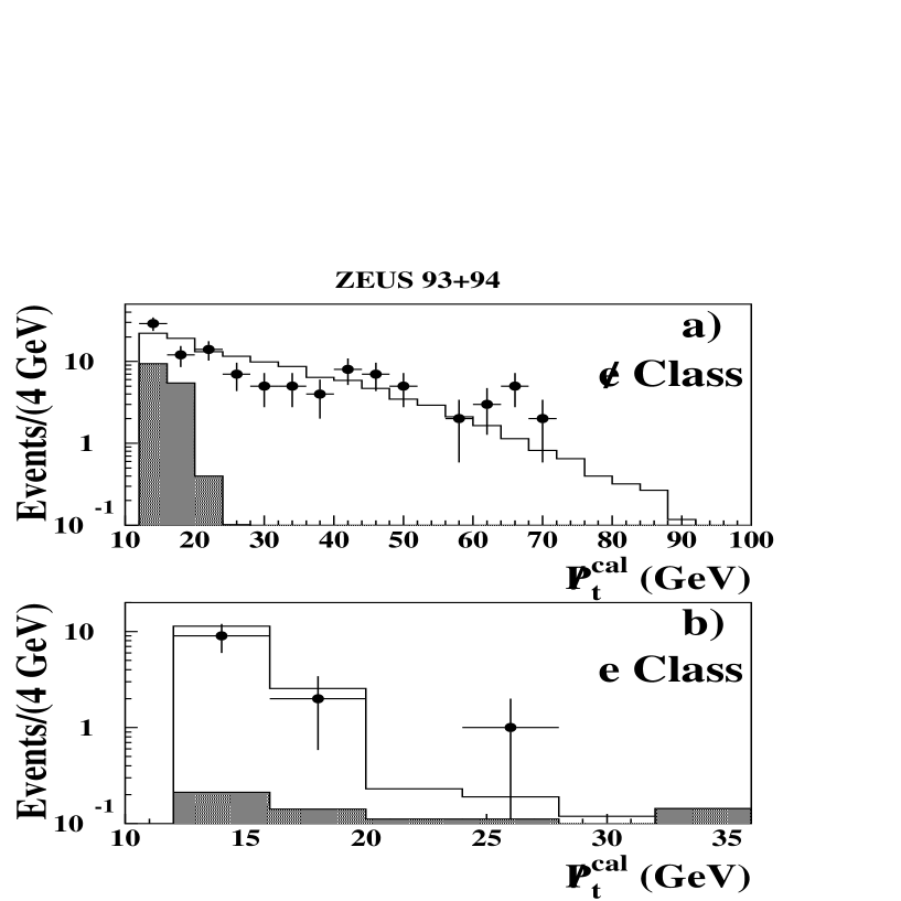
Figure 4: Net transverse momentum ($\not{P}_{t}^{cal}$) distribution of events in the class $\not e$ sample (a) and the class $e$ sample (b). The points represent the data. The solid lines show the Monte Carlo prediction, which includes CC DIS, NC DIS, resolved and direct photoproduction and $\gamma\gamma$ interactions. In the top plot, the shaded region shows the Monte Carlo prediction for all processes except CC DIS. In the bottom plot, the shaded region shows the Monte Carlo prediction for all processes except NC DIS.

There were 114 events with no isolated electron. Six events were rejected because an electron of more than 5 GeV was observed in the luminosity electron calorimeter and they were thus recognized to be background due to photon–proton ($\gamma p$) collisions. This left 108 $\not e$ events, which agrees well with the Monte Carlo estimates of 100 CC DIS events and 15 $\gamma p$ and $\gamma\gamma$ events. The $\not{P}_{t}^{cal}$ distribution of this $\not e$ sample is compared with the Monte Carlo prediction in figure 4a. The $\not e$ sample serves as the source of flavor violation candidates with a muon in the final state, as well as of candidates with final–state $\tau$’s which subsequently decay via $\tau\rightarrow\mu\overline{\nu}\nu$ or $\tau\rightarrow\nu+$hadrons.

$e$:

There were 32 events which contained an isolated electron. In order to reject NC DIS background, for which the electrons are concentrated at large polar angles, we required the electron polar angle to be less than 100^∘. After this cut, 12 events remained in the $e$ sample, compatible with the Monte Carlo prediction of 14 NC DIS events. The $\not{P}_{t}^{cal}$ distribution of these remaining events is compared with the Monte Carlo prediction in figure 4b. LFV candidates with a final–state $\tau$ which decays via $\tau\rightarrow e\overline{\nu}\nu$ (18% branching fraction) were sought in this sample.

The final cuts rely on a clustering algorithm which assigns each calorimeter cell above noise threshold to one and only one cluster. Each cluster is characterized by its energy, $E\mbox{${}_{\scriptscriptstyle clu}$}$, as well as the energy–weighted mean azimuth, $\phi\mbox{${}_{\scriptscriptstyle clu}$}$, and pseudorapidity, $\eta\mbox{${}_{\scriptscriptstyle clu}$}=-\ln[\tan(\theta\mbox{${}_{\scriptscriptstyle clu}$}/2)]$. We expect the final–state lepton in a LFV event to produce a single isolated cluster. To decide if a cluster is isolated, we examine the set of all calorimeter cells which are within 0.8 units in $\eta\phi$ of the cluster ($[(\phi\mbox{${}_{\scriptscriptstyle clu}$}-\phi_{cell})^{2}+(\eta\mbox{${}_{\scriptscriptstyle clu}$}-\eta_{cell})^{2}]^{1/2}<0.8$). A cluster is defined to be isolated if the summed energy of all calorimeter cells in this set which do not belong to the cluster is below 2 GeV. For each cluster, we also compute ${\overline{\phi\mbox{${}_{\scriptscriptstyle clu}$}}}$, which is defined as the energy weighted mean azimuth of all cells in the entire calorimeter, except for those assigned to the cluster. Note that for LFV events ${\overline{\phi\mbox{${}_{\scriptscriptstyle clu}$}}}$ differs only slightly from $\phi\mbox{${}_{\scriptscriptstyle miss}$}$ which is computed using all calorimeter cells. A cluster is said to be $\not{P}_{t}^{cal}$–aligned if it satisfies the inequality: $\cos(\phi\mbox{${}_{\scriptscriptstyle clu}$}-\mbox{${\overline{\phi\mbox{${}_{\scriptscriptstyle clu}$}}}$})<\cos 170^{\circ}$. This ensures that the isolated cluster is opposite in azimuth to the rest of the energy in the calorimeter.

To enter the final sample for $\mu q$ or $\tau q$ final states, an event must satisfy the criteria of one of four selections, described below.

$\mu$ or $\tau\rightarrow\mu$:

In a class $\not e$ event, there must exist an isolated $\not{P}_{t}^{cal}$–aligned cluster with energy 0.5 GeV $<E\mbox{${}_{\scriptscriptstyle clu}$}<6$ GeV and at most 80% of its energy in the electromagnetic layer of the calorimeter. It must have exactly one matching track and that track must have momentum exceeding 20 GeV. The efficiency to satisfy these cuts for scalar (vector) leptoquarks which decay to $\mu q$ decreases with LQ mass from 74% (78%) at $\mbox{$M_{\scriptscriptstyle LQ}$}=80$ GeV to 31% (50%) at $\mbox{$M_{\scriptscriptstyle LQ}$}=260$ GeV. The background estimate for the $\mu$ selection was 0.1 events from the inelastic process $\gamma\gamma\rightarrow\mu^{+}\mu^{-}$. Zero events were observed in the data.

To check the efficiency of the muon selection, we performed an independent event selection which did not use the CAL, but required a track in the barrel or rear muon chambers which was matched to a CTD track with a transverse momentum of at least 5 GeV. In order to select events with isolated muons, we rejected events which had an electron found in the calorimeter or had more than three tracks fitted to the vertex. A total of 15 events, which contained 17 CTD–matched muon chamber tracks passed these cuts. This number agrees with the Monte Carlo estimate of 20 events from $\gamma\gamma\rightarrow\mu^{+}\mu^{-}$. All 17 tracks were matched to an isolated calorimeter cluster which passed the cuts described above (except for the $\not{P}_{t}^{cal}$-alignment).

$\tau\rightarrow e$:

In a class $e$ event, the isolated electron must be $\not{P}_{t}^{cal}$–aligned. The efficiency to satisfy these cuts for scalar (vector) leptoquarks with final–state $\tau q$, and the subsequent decay $\tau\rightarrow e\overline{\nu}\nu$, rises with LQ mass from 23% (17%) at $\mbox{$M_{\scriptscriptstyle LQ}$}=80$ GeV to 75% (75%) at $\mbox{$M_{\scriptscriptstyle LQ}$}=260$ GeV. The background estimate for the $\tau\rightarrow e$ selection was 0.2 events from NC DIS. Zero events were observed in the data.

$\tau\rightarrow$ hadrons:

In a class $\not e$ event, there must exist an isolated $\not{P}_{t}^{cal}$–aligned cluster with $E\mbox{${}_{\scriptscriptstyle clu}$}>10$ GeV, which has either 1 or 3 matching tracks. At least one track must have a momentum exceeding 5 GeV. The efficiency to satisfy these cuts for scalar (vector) leptoquarks with final–state $\tau q$ and hadronic $\tau$ decay rises with leptoquark mass from 15% (12%) at $\mbox{$M_{\scriptscriptstyle LQ}$}=80$ GeV to 39% (47%) at $\mbox{$M_{\scriptscriptstyle LQ}$}=260$ GeV. We estimated a background of 0.4 events for this selection coming from CC DIS (0.2 event), $\gamma\gamma\rightarrow\mu^{+}\mu^{-}$ (0.1 event), and $c{\overline{c}}$ production (0.1 event). We observed zero events.

${\mbox{$\not{P}_{t}^{cal}$}}>80$ GeV:

Leptoquarks with mass in the range 200 GeV$<\mbox{$M_{\scriptscriptstyle LQ}$}<300$ GeV would be strongly boosted in the forward direction so that the final state $\mu$ or $\tau$ would often have polar angle less than 10^∘. In such cases, the final–state lepton would be outside the CTD acceptance and would consequently fail the track matching cuts. In order to maintain high efficiency at these masses, we accept any event from either class $e$ or class $\not e$ for which ${\mbox{$\not{P}_{t}^{cal}$}}>80$ GeV. For 240 GeV leptoquarks which decay to $\mu q$, accepting events with ${\mbox{$\not{P}_{t}^{cal}$}}>80$ GeV increases the overall acceptance from 36% to 69% for scalars, and from 53% to 76% for vectors. For the ${\mbox{$\not{P}_{t}^{cal}$}}>80$ GeV selection, we estimated a background of 1.0 events from CC DIS and we observed zero events.

For the low–mass leptoquark search ($\mbox{$M_{\scriptscriptstyle LQ}$}<300$ GeV), one additional cut was applied, which, in contrast to all cuts described above, depends on $M_{\scriptscriptstyle LQ}$, the mass of the LQ being searched for. The leptoquark mass was reconstructed using the method described in 4.3 and we required that the reconstructed mass must lie within $3\mbox{$\sigma_{\scriptscriptstyle LQ}^{\scriptscriptstyle rec}$}(\mbox{$M_{\scriptscriptstyle LQ}$})$ of $\mbox{$\mu_{\scriptscriptstyle LQ}^{\scriptscriptstyle rec}$}(\mbox{$M_{\scriptscriptstyle LQ}$})$.

5 Results

With no candidate events for LFV found in either the $e^{-}p$ or $e^{+}p$ data samples with integrated luminosities $\mbox{${\cal L}$}_{e^{-}}=0.84$ $pb^{-1}$ and $\mbox{${\cal L}$}_{e^{+}}=2.94$ $pb^{-1}$ , we set upper limits on the couplings of the various LFV processes described in section 2. The upper limit on the coupling $\lambda$ is obtained from the relation $N=\sum_{i=e^{+},e^{-}}\mbox{${\cal L}$}_{i}\epsilon_{i}\sigma_{i}(\lambda)$, where $\epsilon$ is the efficiency, $\sigma(\lambda)$ is the cross section for a coupling $\lambda$, and $N$ is the Poisson 95% confidence level (CL) upper limit [32] on the number of events. The signal efficiencies and background estimates were determined by Monte Carlo studies. We estimate the systematic uncertainties in the efficiencies to be 5%. Cross sections were calculated using the formulae given in the appendix and the GRV–HO [33] parton density parameterization. Cross sections calculated using the MRSH [34] parameterization differ in magnitude by less than 12% for $u$, $d$, $s$, or $c$ quarks in the initial state, and by less than 19% for initial–state $b$ quarks.

5.1 Low-Mass Leptoquark Limits ($M_{LQ}<300$ GeV)

In the case of low–mass leptoquarks, we calculate upper limits on $\lambda_{eq_{1}}^{2}B_{{\ell}q_{2}}$ using equation 2. Since our limits are largely independent of the final state quark type (as long as the top quark is not involved), we show in figures 5 and 6 the upper limits on $\lambda_{eq_{1}}\sqrt{B_{{\ell}q_{2}}}$, for scalar and vector leptoquarks where $q_{1}$ is a first–generation quark and $q_{2}$ is the final–state quark of any generation (except top). The limits for ${\ell}=\mu$ and for ${\ell}=\tau$ are shown separately as a function of LQ mass for the various scalar and vector LQ species. We note that for several LQ species, we probe coupling strengths as small as $\lambda_{eq_{1}}^{2}/4\pi\approx 10^{-3}\alpha$ for $\mbox{$M_{\scriptscriptstyle LQ}$}=100$ GeV and $B_{{\ell}q_{2}}=0.5$.

In figure 7 we compare these limits on LFV with those from previous searches for two representative LQ species, $\tilde{S}_{0}^{R}$ and $V_{0}^{R}$. Assuming that $B_{{\ell}q_{2}}=0.5$, we plot as a solid curve the upper limit on $\lambda_{eq_{1}}$ as a function of the LQ mass. Curves are shown for both $\mu$ (upper plots) and $\tau$ (lower plots) final states. In contrast with many other limits on LFV, the coupling limits from this experiment apply to final–state quarks of any generation (except top). The various broken curves are low–energy limits quoted from reference [10]. For each of these curves, the pairs of numbers in parentheses denote the generations of quarks which couple to $e$ and ${\ell}$. Coupling limits for $B_{{\ell}q}\neq 0.5$ can be obtained by multiplying the limit on $\lambda_{eq_{1}}$ plotted in figure 7 by $\sqrt{0.5/B_{{\ell}q}}$. We emphasize two important implications of figure 7:

1. The ZEUS limits on $ed\rightarrow\mu b$ via $\tilde{S}_{0}^{R}$ ($V_{0}^{R}$) for $\mbox{$M_{\scriptscriptstyle LQ}$}<\sqrt{s}$ supersede previous upper bounds [37] from $B\rightarrow\mu\overline{e}$, for $M_{\scriptscriptstyle LQ}$ below 200 GeV (220 GeV). On the other hand, the limits from $\mu$ conversion in titanium [1] and from forbidden $K$ decays [3] which involve only first and second generation quarks are much stronger than the corresponding ZEUS limits.

2. For $M_{\scriptscriptstyle LQ}$ below 200 GeV, the ZEUS limits on $ed\rightarrow\tau q_{2}$ through $\tilde{S}_{0}^{R}$ and $V_{0}^{R}$ supersede previous limits from $\tau\rightarrow\pi e$ [35], $\tau\rightarrow Ke$ [36], and $B\rightarrow\tau eX$ [37], for $q_{2}=d,s,$ and $b$, respectively.

Figure 7 illustrates examples in which the existing low–energy limits, though less stringent than the ZEUS limits at low $M_{\scriptscriptstyle LQ}$, become more stringent at higher masses. As described in the next section, this is not always the case.

An alternative approach to setting limits, which was employed in reference [7] is to assume that the branching ratio $B_{{\ell}q_{2}}$ is given by $\lambda_{{\ell}q_{2}}^{2}/(\lambda_{eq_{1}}^{2}+\lambda_{{\ell}q_{2}}^{2})$, and to set limits on $\lambda_{{\ell}q_{2}}$ for a fixed value of $\lambda_{eq_{1}}$. Such limits are shown in figure 8. For $F=0$ LQs, our limits are similar to those of reference [7], while for $F=2$ LQs, the ZEUS limits are stronger due to inclusion of $e^{-}p$ data.

Finally, a third way to illustrate the sensitivity is to assume that the LQ couplings have electromagnetic strength ($\lambda_{eq_{1}}^{2}=\lambda_{\mu q_{2}}^{2}=4\pi\alpha$ for LQs which couple to $e$ and $\mu$) and to determine a lower limit on the allowed LQ mass. Such limits are shown in table 1. For scalar leptoquarks, lower mass limits between 207 GeV and 259 GeV are set. Somewhat stronger mass limits, between 219 GeV and 272 GeV, are set on vector leptoquarks for which both the production cross section and detection efficiency are higher.

5.2 High–Mass Leptoquark Limits ($M_{LQ}\gg 300$ GeV)

For high–mass leptoquarks, the cross section is proportional to the square of $\Psi_{eq_{1}{\ell}q_{2}}\equiv\lambda_{eq_{1}}\lambda_{{\ell}q_{2}}/{\mbox{$M_{\scriptscriptstyle LQ}^{2}$}}$, and a factor which does not depend on either the leptoquark couplings or mass (see equations 3 and 4). This is also true of rates for lower energy forbidden processes [10]. For a given limit on $\Psi_{eq_{1}{\ell}q_{2}}$, the limit on the product $\lambda_{eq_{1}}\lambda_{{\ell}q_{2}}$ is proportional to $M_{\scriptscriptstyle LQ}^{2}$. As $M_{\scriptscriptstyle LQ}$ increases, the upper limit on the product of the couplings eventually exceeds unity and the perturbation expansion, on which the formulae in the appendix are based, breaks down. Even so, the parameter $\Psi_{eq_{1}{\ell}q_{2}}$ serves as a reasonable figure of merit for experimental comparisons.

Tables 2, 3, 4 and 5 summarize the 95% CL upper bounds on $\Psi_{eq_{1}{\ell}q_{2}}$, in units of $10^{-4}$ GeV^-2 from this experiment and also from previous experiments [10]. Here $q_{1}$ and $q_{2}$ are the generation indices of the quarks which couple to $e$ and to ${\ell}$ respectively. Two important characteristics of these tables are summarized below.

1. In the $e\leftrightarrow\mu$ case, for LQ species $V_{1/2}^{L}$, $\widetilde{V}_{1/2}^{L}$, $S_{1/2}^{L}$, or $\widetilde{S}_{1/2}^{L}$, the limits from this experiment supersede prior limits in some cases where heavy quark flavors are involved,

2. For the $e\leftrightarrow\tau$ case, we also improve upon existing limits for the same LQ species as in point 1. In addition, because the existing limits on $e\leftrightarrow\tau$ are much weaker than those for $e\leftrightarrow\mu$, the ZEUS limits are the most stringent for several additional LQs which couple to $c$ or $b$ quarks.

5.3 Limits for ${\not{R}_{P}}$ Squarks

Coupling limits for $S_{0}$ and $\tilde{S}_{1/2}$ leptoquarks were converted to coupling limits on ${\tilde{d}}$, ${\tilde{u}}$, and ${\tilde{t}}$ as described in section 2.2. Figure 9 shows 95% CL limits on coupling vs. mass for ${\not{R}_{P}}$ squarks which decay to $\mu q$ and $\tau q$. Here we assume the couplings at the production vertex ($\lambda_{11k}^{\prime}$ for ${\tilde{d}}^{k}$, $\lambda_{1j1}^{\prime}$ for ${\tilde{u}}^{j}$) and at the decay vertex ($\lambda_{ijk}^{\prime}$) to be equal. The solid curves are the ZEUS limits which are given for two assumptions. The lower curves (and the $\tilde{t}$ limits) assume that all squark decays are $R$-parity violating. The upper curves illustrate the impact of gauge decays on the limits. They assume that a single $R$-parity conserving decay, namely ${\tilde{q}}\rightarrow q{\tilde{\gamma}}$ exists and that the photino is much lighter than the squark. Since our analysis is not sensitive to such decays (for which the branching fraction is given by equation 6) these limits are somewhat weaker. The stop mixing angle is assumed to be $\cos^{2}\theta_{t}=0.5$. The dashed curves are limits from low–energy experiments, adapted from reference [10]. Table 6 gives lower mass limits for $\tilde{d}$, $\tilde{u}$, and $\tilde{t}$ assuming that the couplings at the production and decay vertices are equal to the electromagnetic coupling ($\sqrt{4\pi\alpha}$). As with the low–mass leptoquark case described earlier, the ZEUS limits improve on existing limits in cases where quark flavor change accompanies the lepton flavor change, especially for $e\leftrightarrow\tau$ flavor changes.

6 Conclusions

We have searched for signatures of lepton–flavor violation with the ZEUS detector. Hypothetical exotic particles such as leptoquarks could induce lepton–flavor violation observable at HERA. The tight constraints from sensitive searches for processes such as muon conversion in titanium and rare muon and meson decays do not apply to all possible cases of LFV, many of which could be seen in $ep$ collisions. Using 3.8 $pb^{-1}$ of data taken at HERA during the 1993 and 1994 running periods, we have found no candidate events for LFV. The data permit us to constrain specific leptoquark coupling strengths as small as $10^{-3}\alpha$ and to exclude leptoquark masses as large as 270 GeV (for electromagnetic coupling) with 95% confidence. For $\mbox{$M_{\scriptscriptstyle LQ}$}\gg\sqrt{s}$, we calculate upper limits on the product of lepton flavor violating couplings divided by the square of the leptoquark mass, $\lambda_{eq_{1}}\lambda_{{\ell}q_{2}}/\mbox{$M_{\scriptscriptstyle LQ}^{2}$}$, and directly compare these with existing bounds from rare decays. Especially for $e\leftrightarrow\tau$ flavor changes, ZEUS has improved on existing limits for many flavor–violating scenarios.

7 Acknowledgments

We thank the HERA machine group for the excellent machine operation which made this work possible, the DESY computing and network group for providing the necessary data analysis environment, and the DESY directorate for strong support and encouragement. We wish to thank S. Davidson and H. Dreiner for useful discussions.

8 Appendix

We summarize here the cross section formulae [9] for processes involving leptoquarks which couple only to left–handed or right–handed leptons. Process (1) can be mediated by either $s$-channel or $u$-channel leptoquark exchange. For the $s$-channel process, $eq_{1}\to{\ell}q_{2}$, the differential cross section, for unpolarized beams, can be written as:

$$\frac{d^{2}\sigma}{dxdy}=\frac{1}{32\pi xs}q_{1}(x,\mbox{${\hat{s}}$})\frac{\lambda_{eq_{1}}^{2}\lambda_{{\ell}q_{2}}^{2}s^{2}x^{2}}{(sx-\mbox{$M_{\scriptscriptstyle LQ}^{2}$})^{2}+\mbox{$M_{\scriptscriptstyle LQ}^{2}$}\mbox{$\Gamma_{\scriptscriptstyle LQ}^{2}$}}\times\left\{\begin{array}[]{cc}\frac{1}{2}&\mbox{\rm scalar}\;LQ\\ 2(1-y)^{2}&\mbox{\rm vector}\;LQ,\end{array}\right.$$ (7)

where $q_{1}(x,\mbox{${\hat{s}}$})$ is the parton density for the initial state quark or antiquark, $\lambda_{eq_{1}}$ and $\lambda_{{\ell}q_{2}}$ are the couplings at the production and decay vertices, and $\Gamma_{\scriptscriptstyle LQ}$ is the total width of the leptoquark. The partial width for decay into lepton ${\ell}$, and quark $q_{2}$, is

$$\Gamma_{{\ell}q_{2}}=\mbox{$M_{\scriptscriptstyle LQ}$}\lambda_{{\ell}q_{2}}^{2}\times\left\{\begin{array}[]{cc}\frac{1}{16\pi}&{\mbox{\rm scalar}\;LQ}\\ \frac{1}{24\pi}&{\mbox{\rm vector}\;LQ,}\end{array}\right.$$ (8)

so that the typical LQ sought here has $\mbox{$\Gamma_{\scriptscriptstyle LQ}$}\ll\mbox{$M_{\scriptscriptstyle LQ}$}$. In the narrow width approximation, which holds when the variation of $q_{1}(x)$ is small as $x$ is varied by $\delta x\sim\mbox{$\Gamma_{\scriptscriptstyle LQ}$}/\mbox{$M_{\scriptscriptstyle LQ}$}$, integration of equation (7) leads to the formula 2, with $B_{{\ell}q_{2}}=\Gamma_{{\ell}q_{2}}/\mbox{$\Gamma_{\scriptscriptstyle LQ}$}$.

For the $u$-channel process $eq_{2}\to{\ell}q_{1}$, the differential cross section is given by:

$$\frac{d^{2}\sigma}{dxdy}=\frac{1}{32\pi xs}q_{2}(x,-u)\frac{\lambda_{eq_{2}}^{2}\lambda_{lq_{1}}^{2}\,s^{2}\,x^{2}}{\left[sx(1-y)+\mbox{$M_{\scriptscriptstyle LQ}^{2}$}\right]^{2}}\times\left\{\begin{array}[]{cc}\frac{1}{2}(1-y)^{2}&{\mbox{\rm scalar}\;LQ}\\ 2&{\mbox{\rm vector}\;LQ.}\end{array}\right.$$ (9)

In the limit that $\mbox{$M_{\scriptscriptstyle LQ}^{2}$}\gg s$, integration of equations (7) and (9) lead to equations (3) and (4), which are accurate to better than 10% for $\mbox{$M_{\scriptscriptstyle LQ}$}>500$ GeV.

Note that any leptoquark will take part in both $s$- and $u$- channel interactions. For example an $S_{0}^{R}$ leptoquark will mediate the $s$-channel process $e^{+}{\overline{u}}\rightarrow\mu^{+}{\overline{c}}$ as well as the $u$-channel reaction $e^{+}c\rightarrow\mu^{+}u$.

LQ species $$S_{0}^{L}$$

231 242 214 258 259 234 243

223 236 207 253 254 228 236

LQ species

234 243 264 225 254 252 272

227 237 261 219 248 246 270

Table 1: The $95\%$ confidence level lower limits on the LQ mass (GeV) for nominal electromagnetic coupling. For leptoquarks which couple to $\mu$, we set $\lambda_{eq_{1}}^{2}=\lambda_{\mu q_{2}}^{2}=4\pi\alpha$. For leptoquarks which couple to $\tau$, we set $\lambda_{eq_{1}}^{2}=\lambda_{\tau q_{2}}^{2}=4\pi\alpha$. Limits are shown for all scalar (S) and vector (V) leptoquark species.

$$e\leftrightarrow\mu$$                                   

(11)

0.09 0.09 0.12 0.05 0.05 0.03 0.04

(12)

0.14 0.07

0.12 0.12 0.14 0.06 0.09 0.06 0.08

(13)

0.004 0.01 0.004 0.005 0.005

* 0.15 0.07 0.10 0.10 *

(21)

0.14 0.07

0.12 0.12 0.14 0.06 0.05 0.03 0.04

(22)

0.15

0.24 0.24 0.20 0.09 0.10 0.08 0.13

(23)

0.04

* 0.21 0.11 0.13 0.13 *

(31)

0.004 0.01 0.004 0.005 0.005

* 0.16 0.08 0.05 0.05 *

(32)

0.04

* 0.26 0.13 0.11 0.11 *

(33)

0.01 0.01

* 0.29 0.14 0.15 0.15 *

Table 2: The best upper bounds on $\lambda_{eq_{1}}\lambda_{\mu q_{2}}/\mbox{$M_{\scriptscriptstyle LQ}^{2}$}$ for $F=2$ leptoquarks, in units of $10^{-4}$ GeV^-2. Each column corresponds to a given leptoquark species and each row to the quark flavors $q_{1}$ and $q_{2}$ which couple to $e$ and $\mu$, the generation indices of which are specified in the first column. The top line in each box gives the previous measurement [10] which had obtained the strictest limit. The limit from that experiment is given on the second line in the box and the ZEUS limit, shown on the third line, is printed in boldface if it supersedes the previous limit. The asterisks denote those cases where lepton flavor violation occurs only via processes involving top.

$$e\leftrightarrow\mu$$                                   

(11)

0.07 0.06 0.10 0.06 0.06 0.04 0.02

(12)

0.14 0.07

0.08 0.06 0.10 0.07 0.07 0.06 0.03

(13)

0.01 0.01 0.002 0.005 0.002

* 0.11 0.11 0.08 0.08 * 0.08

(21)

0.14 0.07

0.17 0.12 0.17 0.07 0.07 0.06 0.03

(22)

0.07 0.07

0.24 0.16 0.20 0.10 0.10 0.13 0.05

(23)

* 0.21 0.21 0.13 0.13 * 0.13

(31)

0.01 0.01 0.002 0.005 0.002

* 0.20 0.20 0.07 0.07 * 0.07

(32)

* 0.26 0.26 0.11 0.11 * 0.11

(33)

0.001 0.001 0.001

* 0.29 0.29 0.15 0.15 * 0.15

Table 3: The best upper bounds on $\lambda_{eq_{1}}\lambda_{\mu q_{2}}/\mbox{$M_{\scriptscriptstyle LQ}^{2}$}$ for $F=0$ leptoquarks, in units of $10^{-4}$ GeV^-2. Each column corresponds to a given leptoquark species and each row to the quark flavors $q_{1}$ and $q_{2}$ which couple to $e$ and $\mu$, the generation indices of which are specified in the first column. The top line in each box gives the previous measurement [10] which had obtained the strictest limit. The limit from that experiment is given on the second line in the box and the ZEUS limit, shown on the third line, is printed in boldface if it supersedes the previous limit. The asterisks denote those cases where lepton flavor violation occurs only via processes involving top.

$$e\leftrightarrow\tau$$                                   

(11)

0.003 0.02 0.02 0.003 0.01 0.005 0.01

0.15 0.15 0.23 0.09 0.09 0.05 0.06

(12)

0.05 0.03

0.20 0.20 0.27 0.11 0.19 0.13 0.16

(13)

0.004 0.08 0.004 0.04 0.04

* 0.28 0.14 0.23 0.23 *

(21)

0.05 0.03

0.22 0.22 0.31 0.12 0.09 0.05 0.06

(22)

0.5 0.5 0.3 0.1

0.60 0.60 0.48 0.22 0.25 0.19 0.31

(23)

0.04 0.08 0.04 0.04 0.04

* 0.50 0.25 0.33 0.33 *

(31)

0.04 0.08 0.04 0.04 0.04

* 0.34 0.17 0.10 0.10 *

(32)

0.04 0.08 0.04 0.04 0.04

* 0.65 0.32 0.26 0.26 *

(33)

0.3 0.1

* 0.72 0.36 0.38 0.38 *

Table 4: The best upper bounds on $\lambda_{eq_{1}}\lambda_{\tau q_{2}}/\mbox{$M_{\scriptscriptstyle LQ}^{2}$}$ for $F=2$ leptoquarks, in units of $10^{-4}$ GeV^-2. Each column corresponds to a given leptoquark species and each row to the quark flavors $q_{1}$ and $q_{2}$ which couple to $e$ and $\tau$, the generation indices of which are specified in the first column. The top line in each box gives the previous measurement [10] which had obtained the strictest limit. The limit from that experiment is given on the second line in the box and the ZEUS limit, shown on the third line, is printed in boldface if it supersedes the previous limit. The asterisks denote those cases where lepton flavor violation occurs only via processes involving top.

$$e\leftrightarrow\tau$$                                   

(11)

0.02 0.01 0.02 0.002 0.01 0.01 0.002

0.11 0.09 0.18 0.11 0.11 0.07 0.04

(12)

0.05 0.03 0.03

0.12 0.10 0.18 0.15 0.15 0.10 0.05

(13)

0.08 0.08 0.02 0.04 0.02

* 0.18 0.18 0.16 0.16 * 0.16

(21)

0.05 0.03 0.03

0.34 0.26 0.39 0.14 0.14 0.10 0.05

(22)

0.2 0.2

0.60 0.37 0.48 0.25 0.25 0.31 0.13

(23)

0.08 0.08 0.02 0.04 0.02

* 0.50 0.50 0.33 0.33 * 0.33

(31)

0.08 0.08 0.002 0.04 0.002

* 0.47 0.47 0.15 0.15 * 0.15

(32)

0.08 0.08 0.02 0.04 0.02

* 0.65 0.65 0.26 0.26 * 0.26

(33)

3.4 3.4

* 0.72 0.72 0.38 0.38 * 0.38

Table 5: The best upper bounds on $\lambda_{eq_{1}}\lambda_{\tau q_{2}}/\mbox{$M_{\scriptscriptstyle LQ}^{2}$}$ for $F=0$ leptoquarks, in units of $10^{-4}$ GeV^-2. Each column corresponds to a given leptoquark species and each row to the quark flavors $q_{1}$ and $q_{2}$ which couple to $e$ and $\tau$, the generation indices of which are specified in the first column. The top line in each box gives the previous measurement [10] which had obtained the strictest limit. The limit from that experiment is given on the second line in the box and the ZEUS limit, shown on the third line, is printed in boldface if it supersedes the previous limit. The asterisks denote those cases where lepton flavor violation occurs only via processes involving top.

	$\tilde{d}\rightarrow\mu q$	$\tilde{u}\rightarrow\mu q$	$\tilde{t}\rightarrow\mu q$	$\tilde{d}\rightarrow\tau q$	$\tilde{u}\rightarrow\tau q$	$\tilde{t}\rightarrow\tau q$
50% gauge decays	217	223	-	209	216	-
no gauge decays	231	234	223	223	228	216

Table 6: 95% CL mass limits (GeV) for squarks with ${\not{R}_{P}}$-couplings, of electromagnetic strength ($\lambda_{11k}^{2}=\lambda_{ijk}^{2}=4\pi\alpha=4\pi/128$). The first line gives the mass limits for the case where the total branching fraction for gauge decays is 50%, the second line gives the mass limits for a squark which always has ${\not{R}_{P}}$ decays. The limits which assume 50% gauge decays are weaker because we did not search for the gauge decays. The mixing angle of the stop is assumed to be $\cos^{2}\theta_{t}=0.5$.

Figure 1: The (a) $s$–, (b) $u$–, and (c) $t$–channel Feynman diagrams for LFV. For the $s$–channel and $u$–channel diagrams, we denote the couplings as $\lambda_{{\ell}q}$, where the indices refer to the lepton and quark flavors.

Figure 2: Existing 95% CL limits [10] on the product of the couplings $\lambda_{eq_{1}}\lambda_{{\ell}q_{2}}$ vs. leptoquark mass $M_{\scriptscriptstyle LQ}$ for a $S_{0}^{L}$ leptoquark mediating $e\leftrightarrow\mu$ and $e\leftrightarrow\tau$ transitions accompanied by various quark flavor changes. Each limit curve excludes the region above it. The vertical lines indicate lower limits of allowed leptoquark mass from LEP [11] and the Tevatron [12]. The Tevatron limits apply to any scalar leptoquark which couples to $\mu$ and depend on the branching fractions $B_{\mu}$ to the $\mu q$ final state. The limits are shown for $B_{\mu}$ equal to 0.5 and 1.

Figure 3: $R_{P}$ violating single squark production in $ep$ collisions. Diagrams a) and b) show production of ${\tilde{u}}$ and ${\tilde{d}}$ squarks with leptoquark–like ${\not{R}_{P}}$ decays, where ${\ell}^{i}$ denotes the final–state charged lepton of generation $i$. The indices $j$ and $k$ denote the generations of up–type and down–type (s)quarks respectively. Diagram c) shows ${\tilde{u}}$ production with an $R_{P}$–conserving decay.

Figure 5: The upper limit on the coupling at the production vertex ($\lambda_{eq_{1}}$) times the square root of the branching fraction to the $\mu q$ or $\tau q$ final state ($B_{{\ell}q_{2}}$) vs. leptoquark mass $M_{LQ}$, at $95\%$ CL for scalar leptoquarks. The horizontal line indicates nominal electromagnetic coupling ($\lambda_{eq_{1}}^{2}=4\pi\alpha=4\pi/128$) and $B_{{\ell}q_{2}}=0.5$.

Figure 6: The upper limit on the coupling at the production vertex ($\lambda_{eq_{1}}$) times the square root of the branching fraction to the $\mu q$ or $\tau q$ final state ($B_{{\ell}q_{2}}$) vs. leptoquark mass $M_{LQ}$, at $95\%$ CL for vector leptoquarks. The horizontal line indicates nominal electromagnetic coupling ($\lambda_{eq_{1}}^{2}=4\pi\alpha=4\pi/128$) and $B_{{\ell}q_{2}}=0.5$.

Figure 7: The $95\%$ CL upper limits on $\lambda_{eq_{1}}$ vs. leptoquark mass $M_{LQ}$, for selected LQ species which decay to ${\ell}q$, where ${\ell}=\mu$ (above) or $\tau$ (below), assuming $B_{{\ell}q_{2}}=0.5$. The solid curves are ZEUS results and the various broken curves show existing limits [10]. Paired numbers in parentheses indicate the generations of the quarks which couple to $e$ and ${\ell}$ respectively.

Figure 8: The upper limit on the coupling at the decay vertex ($\lambda_{{\ell}q_{2}}$) vs. leptoquark mass $M_{LQ}$, for several values of the first–generation coupling at the production vertex ($\lambda_{eq_{1}}$). Each curve is labeled by the value of $\lambda_{eq_{1}}$. The dotted curves are for $F=2$ leptoquarks and the solid curves are for $F=0$ leptoquarks.

Figure 9: Limits on the ${\not{R}_{P}}$ coupling $\lambda^{\prime}_{ijk}$ at $95\%$ CL for squarks which decay to $\mu q$ ($i=2$) or $\tau q$ ($i=3$). For ${\tilde{d}}$ limits, we assume that $\lambda_{11k}^{\prime}=\lambda_{ijk}^{\prime}$, while for ${\tilde{u}}$ (including ${\tilde{t}}$) limits, we assume that $\lambda_{1j1}^{\prime}=\lambda_{ijk}^{\prime}$. The lower solid curves give the ZEUS limits for squarks which decay purely via $R$-parity violation. The upper solid curves give the ZEUS limits for the case where, in addition, the gauge decay $\tilde{q}\to q{\tilde{\gamma}}$ exists, and where the photino is much lighter than the squark. In the case of ${\tilde{t}}$, we only consider ${\not{R}_{P}}$ decays and assume that the stop mixing angle is given by $\cos^{2}\theta_{t}=0.5$. The values of $j$ and $k$ for which each limit applies are indicated above the plots. The dashed and dotted curves show the limits from other experiments (adapted from [10]). These limits depend on the generation of the quark which couples to the $\mu$ or $\tau$ as indicated.

References

-
[1]
S. Ahmad et al., Phys. Rev. D38 (1988) 2102 ;
T. Kosmas et al., Nucl. Phys. A570 (1994) 637. - [2] A. van der Schaff, Progress in particle and nuclear physics, 31 (1993) 1.
- [3] L.M. Sehgal, PITHA-94-52 (1994) 1.
- [4] H. Kroha, Mod. Phys. Lett. A8 (1993) 869.
- [5] I.I. Bigi, G. Köpp, and P.M. Zerwas, Phys. Lett. 166B (1986) 238.
- [6] S. Yang, Ph.D. thesis, Columbia University, CU-95-396 (1995).
- [7] H1 Coll., S. Aid et al., Phys. Lett 369B (1996) 173.
- [8] B. Schrempp, Proc. of the 1991 Workshop on Physics at HERA, ed. W. Buchmüller and G. Ingelman, (DESY, Hamburg 1992), p.1034, and references therein.
- [9] W. Buchmüller, R. Rückl, and D. Wyler, Phys. Lett. 191B (1987) 442.
- [10] S. Davidson, D. Bailey, and B. Campbell, Z. Phys. C61 (1994) 613.
-
[11]
L3 Coll., B. Adeva et al., Phys. Lett. 261B (1991) 169;
OPAL Coll., G. Alexander et al., Phys. Lett. 263B (1991) 123;
DELPHI Coll., P. Abreu et al., Phys. Lett. 316B (1993) 620. -
[12]
CDF Coll., F. Abe et al., Phys. Rev. Lett. 75 (1995) 1012;
D0 Coll., S. Abachi et al., Phys. Rev. Lett. 75 (1995) 3618. - [13] V. Barger, G.F. Giudice, and T. Han, Phys. Rev. D40 (1989) 2987.
- [14] J. Butterworth and H. Dreiner, Nucl. Phys. B397 (1993) 3, and references therein.
-
[15]
T. Kon and T. Kobayashi, Phys. Lett. B270 (1991) 81;
T. Kon, T. Kobayashi and K. Nakamura, Proc. of the 1991 Workshop on Physics at HERA, ed. W. Buchmüller and G. Ingleman, (DESY, Hamburg 1992), p.1088. - [16] The ZEUS Detector, Status Report 1993, DESY 1993.
-
[17]
M. Derrick et al., Nucl. Inst. Meth. A309 (1991) 77;
A. Andresen et al., Nucl. Inst. Meth. A309 (1991) 101;
A. Bernstein et al., Nucl. Inst. Meth. A336 (1993) 23;
A. Caldwell et al., Nucl. Inst. Meth. A321 (1992) 356. -
[18]
N.Harnew et al., Nucl. Inst. Meth. A279(1989)290;
B.Foster et al., Nucl. Phys., Proc. Suppl. B32(1993);
B.Foster et al., Nucl. Inst. Meth. A338(1994)254 - [19] G. Abbiendi et al., Nucl. Inst. Meth. A333 (1993) 342.
- [20] J. Andruszków et al., DESY 92–066 (1992).
- [21] PYTHIA 5.6 and JETSET 7.4, H.U. Bengtsson, T. Sjöstrand, Comp. Phys. Comm. 46 (1987) 43.
- [22] LEPTO 6.1, G. Ingelman, Proc. of the 1991 Workshop on Physics at HERA, ed. W. Buchmüller and G. Ingleman, (DESY, Hamburg 1992), p.1366.
- [23] HERACLES 4.1, A. Kwiatkowski, H. Spiesberger and H.J. Möhring, Proc. of the 1991 Workshop on Physics at HERA, ed. W. Buchmüller and G. Ingleman, (DESY, Hamburg 1992), p.1294.
- [24] DJANGO 6.1, G. Schuler et al., Proc. of the 1991 Workshop on Physics at HERA, ed. W. Buchmüller and G. Ingleman, (DESY, Hamburg 1992), p.1419.
- [25] A.D. Martin, W.J. Stirling, and R.G. Roberts, Phys. Rev. D50 (1994) 6734.
-
[26]
ARIADNE 4.03, L. Lönnblad, LU TP–89–10 (1989);
L. Lönnblad, Comp. Phys. Comm. 71 (1992) 15. - [27] HERWIG 5.8, G. Marchesini et al., Comp. Phys. Comm. 67 (1992) 465.
- [28] AROMA 2.1, G. Ingelman and G. Schuler, Proc. of the 1991 Workshop on Physics at HERA, ed. W. Buchmüller and G. Ingleman, (DESY, Hamburg 1992), p.1346.
- [29] A generator based on J.A.M. Vermaseren, Nucl. Phys. B229 (1983) 347.
- [30] U. Baur, J.A.M. Vermaseren, and D. Zeppenfeld, Nucl. Phys. B375 (1992) 3.
- [31] R. Brun et al., CERN DD/EE–84–1 (1987).
- [32] L. Montanet et al., Review of Particle Properties, Phys. Rev. D50 (1994) 1173 (see p. 1281).
- [33] M. Glück, E. Reya, and Vogt, Z. Phys. C53 (1992) 127.
- [34] A.D. Martin, W.J. Stirling, R.G. Roberts, RAL–93–077 (1993).
- [35] Crystal Ball Coll., S. Keh et al., Phys. Lett. B212 (1988) 123.
- [36] K.G. Hayes et al., Phys. Rev. D25 (1982) 2869.
- [37] CLEO Coll., R. Ammar et al., Phys. Rev. D49 (1994) 5701.
- [38] Private communications with S. Davidson.