UR-1494
April, 1997
hep-ex/9704017

STATUS OF WEAK QUARK MIXING^†

Lawrence K. Gibbons

Department of Physics and Astronomy, University of Rochester
Rochester, NY 14627, USA

Abstract

The experimental status of the Cabibbo-Kobayashi-Maskawa matrix is reviewed. Measurements discussed include $B^{0}_{(s)}-\bar{B}^{0}_{(s)}$ mixing and several rare $B$ and $K$ decays with implications for $|V_{td}|$ and $|V_{ts}|$. Extraction of $|V_{cb}|$ and $|V_{ub}|$ from studies of semileptonic $B$ decay is also discussed.

^†Invited talk given at the 28th International Conference on High Energy Physics, Warsaw, Poland, 25-31 July 1996, to appear in the proceedings.

Abstract

The experimental status of the Cabibbo-Kobayashi-Maskawa matrix is reviewed. Measurements discussed include $B^{0}_{(s)}-\bar{B}^{0}_{(s)}$ mixing and several rare $B$ and $K$ decays with implications for $|V_{td}|$ and $|V_{ts}|$. Extraction of $|V_{cb}|$ and $|V_{ub}|$ from studies of semileptonic $B$ decay is also discussed.

1 Introduction

This review summarizes the status of weak quark mixing, focusing on our knowledge of the Cabibbo-Kobayashi-Maskawa (CKM) matrix [1, 2] elements $V_{cb}$, $V_{ub}$, $V_{td}$ and $V_{ts}$. Precise evaluation of these elements is crucial to our understanding of the origins of $CP$ violation — in particular, whether the $CP$–violating phase of the CKM matrix is sufficient to explain the observed rate of the $CP$-violating decay $K_{L}\to\pi\pi$.

The results discussed here are intimately connected with topics covered in more detail in three other talks. To extract the CKM elements, we must understand the dynamics underlying the decays studied; J. Richman [4] and G. Martinelli [5] discuss the dynamics in detail. The elements under discussion are the basic inputs to the “Unitarity Triangle” (UT) analysis to test the hypothesis that the rate of $CP$ violation observed in the neutral kaon system is consistent with arising solely from a $CP$–violating phase in the CKM matrix. A. Buras [6] will present a detailed UT analysis in his talk.

The CKM matrix appears in the weak charged current,

$$J_{\mu}=(\bar{u}\bar{c}\bar{t})_{L}\gamma_{\mu}\left(\!\!\begin{array}[]{rrr}V_{ud}&V_{us}&V_{ub}\\ V_{cd}&V_{cs}&V_{cb}\\ V_{td}&V_{ts}&V_{tb}\end{array}\!\!\right)\left(\!\!\begin{array}[]{c}d\\ s\\ b\end{array}\!\!\right)_{L},$$ (1)

rotating the quark system from the flavor eigenstate basis to the weak eigenstate basis. A convenient parameterization, due to Wolfenstein [3], in which the matrix is expanded in powers of the Cabibbo angle $\lambda=|V_{td}|=0.22$ is

$$V_{\scriptscriptstyle CKM}\approx$$ (6)

$$\!\!\!\left(\!\!\begin{array}[]{ccc}1-\lambda^{2}/2&\lambda&A\lambda^{3}(\rho-i\eta)\\ -\lambda&1-\lambda^{2}/2&A\lambda^{2}\\ A\lambda^{3}(1-\rho-i\eta)&-A\lambda^{2}&1\end{array}\!\!\!\right).$$

Within this approximation, good to order ${\cal O}(\lambda^{3})$, $CP$–violating amplitudes are proportional to the parameter $\eta$. Buras [6] discusses both this parameterization and the unitary triangle that results from the unitary property $\sum V_{ik}V^{*}_{jk}=0$ for $i\neq j$ in some detail.

Section 2 of this review will discuss experimental measurements sensitive to $|V_{td}|$ and $|V_{ts}|$. Section 3 will summarize the determination of $|V_{cb}|$ from inclusive and exclusive $b\to c\ell\nu$ decays, while section 4 will focus on the new determination of $|V_{ub}|$ from exclusive $B\to X_{u}\ell\nu$ studies.

2 $V_{td}$ and $V_{ts}$

The top quark presents an experimental irony. Its large mass and short lifetime make possible an accurate determination of its mass with only a handful of events. In fact, its mass is fractionally among the best determined for any quark. However, the large mass limits us to a total event sample of only a few events, making direct determination of $|V_{td}|$ and $|V_{ts}|$ impossible at this time. We must therefore resort to indirect means of determining those CKM elements.

Weak processes that contain a virtual top quark in a loop provide such a means. Because the amplitudes are roughly proportional to the square of the large top quark mass, such processes can have accessible rates. In fact, the large rate observed in the initial $B^{0}-\bar{B}^{0}$ mixing measurements [7] was the first hint that the top quark was unusually heavy. Figure 1 shows a variety of these processes. Electroweak penguin diagrams contribute to the decays $B\to K^{*}\gamma$, $B\to\rho\gamma$ and $K^{+}\to\pi^{+}\nu\bar{\nu}$. The box diagram, a second order weak process, also contributes to the decay $K^{+}\to\pi^{+}\nu\bar{\nu}$, as well as to $B^{0}-\bar{B}^{0}$ and $B^{0}_{s}-\bar{B}^{0}_{s}$ mixing. The experimental status for these four different processes follows, with a summary of the implications for $|V_{td}|$ and $|V_{ts}|$ at the end of this section.

Figure 1: Diagrams for processes from which information about $V_{td}$ and $V_{ts}$ can be inferred: $K^{+}\to\pi^{+}\nu\bar{\nu}$ (left), $B\to K^{*}(\rho)\gamma$ (top right), and $B^{0}-\bar{B}^{0}$ mixing (bottom right).

2.1 $K^{+}\to\pi^{+}\nu\bar{\nu}$

Theoretically, one of the cleanest avenues for the extraction of $|V_{ts}|$ is the semileptonic decay $K^{+}\to\pi^{+}\nu\bar{\nu}$. Long distance corrections have been found to be negligible [8, 9] compared to the short distance contribution from diagrams like those in Figure 1. Uncertainties in the hadronic current can be eliminated by normalizing to the related semileptonic decay $K^{+}\to\pi^{0}e^{+}\nu$. For this decay, while the amplitudes of diagrams containing the top quark are enhanced by its large mass, they also contain the factor $V_{ts}^{*}V_{td}$, of order $\lambda^{5}$. On the other hand, the amplitudes from analogous diagrams with a charm quark in the loop contain the factor $V_{cs}^{*}V_{cd}$, of order $\lambda$, making the charmed loops competitive with the top. The charm quark contribution still accounts for the largest theoretical uncertainty, though that uncertainty has recently been greatly reduced to about 4% by a next-to-leading order calculation of Buchalla and Buras [10]. Within the standard model, predictions [6] for this decay rate lie in the range $(0.6-1.2)\times 10^{-10}$.

Figure 2: Schematic of the upgraded E787 detector.

The Brookhaven experiment E787 has been searching for this decay with an elegant detector, shown in its current upgraded form in Figure 2. A high intensity beam from the AGS delivers $K^{+}$ mesons, which are tagged in a Čerenkov counter, slowed and then stopped in an active segmented target. Charged particles from the target are tracked in a drift chamber and range out in a segmented range stack of plastic scintillator layers. Having instrumented all active channels with transient digitizers, E787 can suppress background from $K^{+}\to\mu^{+}\nu$ decays (63% branching fraction) by identifying the complete decay sequence $\pi^{+}\to\mu^{+}\to e^{+}$. Photon vetos suppress $\pi^{+}\pi^{0}$ decays (21% branching fraction). Candidate $\pi^{+}$ are selected in a momentum range between the two peaks from $\mu^{+}\nu$ and $\pi^{+}\pi^{0}$ decays. The final data distribution [11] in range ($R$) versus kinetic energy ($T$) measured in the range stack is shown in Figure 3 for the 1989-1991 runs. No events are observed in the signal region. From this data E787 has set the 90% C.L. upper limit ${\cal B}(K^{+}\to\pi^{+}\nu\bar{\nu})<2.4\times 10^{-9}$.

Figure 3: Range ($R_{\pi}$) versus kinetic energy ($T_{\pi}$) for events satisfying the E787 selection criteria and $211\leq p_{\pi}\leq 243$ MeV/$c$. The box indicates the $K^{+}\to\pi^{+}\nu\bar{\nu}$ search region. $K^{+}\to\pi^{+}\pi^{0}$ background populates the lower left region; $K^{+}\to\mu^{+}\nu$ populates the upper right.

The E787 experiment has been accumulating more data with its upgraded detector. The upgrade has resulted in a detector with lower mass and better light collection, and hence with better $\pi/\mu$ separation in both $T$ and $R$ and with improved photon vetoing. After initial runs in 1995 and 1996, E787 estimates a factor of six improvement in reach over their previous data set. After completing their planned 1997 run, they expect a final sensitivity of about $2\times 10^{-10}$. The theoretical uncertainties in this mode are small enough that a signal at this level would be a strong indication of physics beyond the standard model.

2.2 $B\to K^{*}\gamma$, $B\to\rho\gamma$

Study of the exclusive radiative penguin decays $B\to K^{*}\gamma$ and $B\to\rho\gamma$ can play several roles in constraining CKM elements. Foremost is the extraction of the ratio $|V_{td}/V_{ts}|$ from the ratio of branching fractions $R\equiv{\cal B}(B\to\rho\gamma)/{\cal B}(B\to K^{*}\gamma)$, though one must correct for differences in phase space, $SU(3)$-breaking, and, particularly for $\rho\gamma$, long distance (LD) contributions

Recent estimates have indicated that the long distance contributions may be manageable: of order [12, 13] 10% for $B^{-}\to\rho^{-}\gamma$, and a few percent [14] or less for $B^{0}\to\rho^{0}/\omega\gamma$. The question, however, is still under active investitarion. The phase space correction [15] is small, $1.02\pm 0.02$. The $SU(3)$-breaking correction $\xi$ is model-dependent, but this dependence should be smaller than for predictions of the individual $\rho\gamma$ and $K^{*}\gamma$ rates. Calculations [15, 16, 17] of $\xi$ range from 0.58 to 0.90.

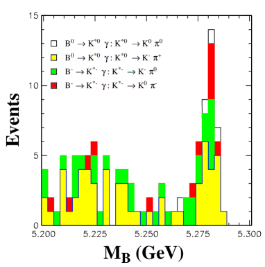
Figure 4: Reconstructed mass distribution of $B\to K^{*}\gamma$ candidates in the four modes studied at CLEO.

CLEO [18] has recently updated its measurements of $B\to K^{*}\gamma$ and placed new upper limits on $B^{-}\to\rho^{-}\gamma$ and $B^{0}\to\rho^{0}/\omega\gamma$. A strong signal can be seen in the sum of the four $K^{*}\gamma$ modes examined (Figure 4), and combined they yield ${\cal B}(B\to K^{*}\gamma)=(4.2\pm 0.8\pm 0.6)\times 10^{-5}$. CLEO sees no evidence for a signal in any of the three $b\to d\gamma$ modes studied. Combining the $K^{*}\gamma$ measurement with these three modes under the assumption that $\Gamma(B^{-}\to\rho^{-}\gamma)=2\Gamma(B^{0}\to\rho^{0}/\omega\gamma)$, CLEO obtains the 90% C.L. upper limit $R<0.19$. Assuming no long distance contribution to any of the $b\to d\gamma$ modes, but correcting for phase space and $SU(3)$–breaking, this limit implies $|V_{td}/V_{ts}|<0.45-0.56$, where the range comes from the different predictions for $\xi$. Allowing for a 10% long distance amplitude for $B^{-}\to\rho^{-}\gamma$ that, to be conservative, interferes destructively, the limit’s upper range would change to $|V_{td}/V_{ts}|<0.59$.

2.3 $B^{0}-\bar{B}^{0}$ mixing

The formalism for mixing of neutral $B$ mesons, either $B_{s}$ or $B_{d}$, is completely analogous to that of neutral $K$ mesons. The weak eigenstates are a mixture of the flavor $\left|B^{0}\right>$ and $\left|\bar{B}^{0}\right>$ eigenstates:

$$\left|B_{S}\right> = p\left|B^{0}\right>+q\left|\bar{B}^{0}\right>,$$

$$\left|B_{L}\right> = p\left|B^{0}\right>-q\left|\bar{B}^{0}\right>,$$ (7)

with the complex amplitudes $p$ and $q$ normalized such that $|p|^{2}+|q|^{2}=1$. The labeling of the weak neutral $B$ eigenstates analogously to their kaon counterparts is somewhat of a misnomer. For a neutral meson $H$, the only contribution to the lifetime difference of the weak eigenstates comes from final states that are common to both $H^{0}$ and $\bar{H}^{0}$. In the case of the kaon, the $\pi\pi$ final states are by far the dominant final state, and their contribution leads to a $K_{L}$ lifetime about 580 times larger than the $K_{S}$ lifetime. In the case of the $B$ mesons [19], the branching fractions of final states common to both the $B^{0}$ and $\bar{B}^{0}$ are only of order $10^{-3}$, and different final states will contribute to the width with different signs. Hence the lifetime difference $\Delta\Gamma=\Gamma_{L}-\Gamma_{S}$ is expected to be quite small, with $|\Delta\Gamma|/\Gamma$ of order a few percent or less.

In the $B^{0}_{d}-\bar{B}^{0}_{d}$ system, where the branching fractions for a large number of decay modes have been measured, the common final states do have small branching fractions. This is expected to be the case in the $B^{0}_{s}-\bar{B}^{0}_{s}$ system as well. I will assume that $\Delta\Gamma=0$, as the experiments do, which implies [19] that the ratio $|p/q|=1$.

Processes such as the box diagrams in Figure 1 do generate a mass difference, $\Delta m\equiv M_{B_{L}}-M_{B_{S}}$, just as in the neutral kaon system. Given this mass difference, an initially pure $B^{0}$ or $\bar{B}^{0}$ state evolves as a function of proper time according to

$$\left|B^{0}(t)\right>=e^{-t(\frac{\Gamma}{2}+iM)}\times$$

$$\left[\cos(\frac{\Delta mt}{2})\left|B^{0}\right>+\frac{iq}{p}\sin(\frac{\Delta mt}{2})\left|\bar{B}^{0}\right>\right]$$

$$\left|\bar{B}^{0}(t)\right>=e^{-t(\frac{\Gamma}{2}+iM)}\times$$

$$\left[\cos(\frac{\Delta mt}{2})\left|\bar{B}^{0}\right>+\frac{ip}{q}\sin(\frac{\Delta mt}{2})\left|B^{0}\right>\right],$$

where $M\equiv(M_{L}+M_{S})/2$. The probability as a function of proper time that an initially pure $B^{0}$ or $\bar{B}^{0}$ state decay as the opposite, or “mixed”, state is

$${\cal P}_{m}(t)=\frac{\Gamma}{2}e^{-\Gamma t}[1-\cos(\Delta mt)]$$ (9)

and as the same, unmixed state is

$${\cal P}_{u}(t)=\frac{\Gamma}{2}e^{-\Gamma t}[1+\cos(\Delta mt)].$$ (10)

These forms result when $\Delta\Gamma=0$, and hence $|p/q|=1$, without assuming strict $CP$-conservation. Integrated over time, the total fraction $\chi_{q}$ of mixed decays from an initially pure $B_{q}$ state is given by

$$\chi_{q}=\int_{0}^{\infty}{\cal P}_{m}(t)\,dt=\frac{x_{q}^{2}}{2(1+x_{q}^{2})},$$ (11)

where $x_{q}=\Delta m_{q}/\Gamma_{q}$.

The ultimate experimental goal is a precise determination of the mass differences $\Delta m_{d}$ and $\Delta m_{s}$, from which we can obtain information concerning $V_{td}$ and $V_{ts}$. Within the Standard Model, the box diagrams with a top quark in the internal loop dominate the contribution to the mass difference. Their evaluation for either the $B_{d}$ ($q=d$) or $B_{s}$ ($q=s$) system yields [20]

$$\Delta m_{q}=\frac{G_{F}^{2}}{6\pi^{2}}B_{B_{q}}f_{B_{q}}^{2}M_{B_{q}}m_{t}^{2}|V_{tb}^{*}V_{tq}|^{2}\eta_{B}\frac{S(x_{t})}{x_{t}},$$ (12)

where $x_{t}=(m_{t}/M_{W})^{2}$ and $S(x_{t})$ is the Inami-Lim function that results from evaluation of the box diagrams with internal top quarks [21]. A good working approximation [23] to $S(x_{t})$ is

$$S(x_{t})=0.784\,x_{t}^{0.76}.$$ (13)

Buras et al. [22] have evaluated the QCD correction factor $\eta_{B}=0.55$, which is the same for $B_{d}$ and $B_{s}$ mixing [23]. They also stress that the running top mass $\bar{m}_{t}(m_{t})$, not the pole mass, should be used in the evaluation of (12). From the precise determination [24] of $m_{t}=175\pm 6$ by CDF and D0, Buras obtains [6] $\bar{m}_{t}(m_{t})=167\pm 6$ GeV.

With the top quark mass now so well known, the largest uncertainties in the evaluation of (12) arise from the dearth of precise knowledge about $f_{B}$, the $B$ decay constant, and $B_{B}$, the nonperturbative correction factor. Flynn [25] has summarized the lattice calculations of both quantities for the $B_{d}$ system. I will use Buras’ evaluation [26] of results from lattice, QCD sum rule and QCD dispersion relation calculations:

$$f_{B_{d}}\sqrt{B_{B_{d}}}=200\pm 40\,\,{\rm MeV}.$$ (14)

Many of the calculational uncertainties are reduced if one considers the ratio

$$\xi=\frac{f_{B_{s}}\sqrt{B_{B_{s}}}}{f_{B_{d}}\sqrt{B_{B_{d}}}}.$$ (15)

Thus the ratio

$$\frac{\Delta m_{s}}{\Delta m_{d}}=\xi^{2}\frac{M_{B_{s}}}{M_{B_{d}}}\left|\frac{V_{ts}}{V_{td}}\right|^{2}$$ (16)

provides a powerful way to obtain $|V_{ts}/V_{td}|$. Both quenched lattice calculations, summarized here by Flynn [25], and QCD sum rule calculations [27, 28] are consistent with $\xi=1.15\pm 0.05$. With this precision, we shall see that even the current limit on $\Delta m_{s}$ begins to provide interesting constraints in Unitary Triangle analyses. One word of caution, however. Flynn does note that the unquenching of lattice calculations is likely to increase $\xi$, perhaps by as much as 10%. Values as large as 1.25-1.30 can not be discounted.

Figure 5: Probability distributions ${\cal P}_{u}(t)$ (solid) and ${\cal P}_{m}(t)$ (dashed) for an initially pure $B^{0}_{d}$ or $\bar{B}^{0}_{d}$ state and for a state that does not mix (dotted). Inset: the fraction of decays from the mixed state as a function of proper time.

This review focuses on measurements that are sensitive to the time dependence of ${\cal P}_{m}(t)$, and hence extract $\Delta m$ directly from the observed time-dependence. Figure 5 illustrates the behavior of the $B_{d}$ system; the time-dependent measurements examine variables proportional to the fraction of mixed events as a function of proper time. Because $x_{d}=\Delta m_{d}/\Gamma_{d}\sim 0.75$, measurements are sensitive to roughly the end of the first $1/2$ cycle (about 6.5 ps), where the decay rate has decreased by a factor of 65.

For the $B_{s}$ system, the lower limits on $\Delta m_{s}$ imply that $\chi_{s}$ will be very close to the limit $0.5$. Hence, accurate determination of $x_{s}$ from measurement of the total mixed fraction $\chi_{s}$ is not practical. A large $\Delta m_{s}$ means a rapid oscillation frequency — for $\Delta m_{s}\sim 10\,\hbar\,{\rm ps}^{-1}$, the half cycle would be about $0.3{\rm\,ps}$. This is about the current experimental time resolution, making determination of $\Delta m_{s}$ a challenge on all fronts!

2.3.1 $B_{d}-\bar{B}_{d}$ mixing

The LEP experiments have done an extraordinary job of determining $\Delta m_{d}$. The techniques will be described briefly, with note to novel features of new analyses from SLAC and CDF. Wu [29] has reviewed the LEP measurement techniques in greater detail than possible here.

For a time-dependent mixing measurement one must measure the $B$ proper time $t=LM_{B}/p_{B}$. The large boosts of the $B$ mesons and the silicon vertex detectors at the LEP experiments, at SLD and at CDF make the measurement of the decay length $L$ with the requisite precision possible.

Generally, the decay length $L$ is reconstructed by (i) reconstructing a tertiary charm vertex, either inclusively (eg., with a topological algorithm) or via an exclusive $D$ channel, (ii) extrapolating the reconstructed $D$ back to form a vertex with a track, such as a high $p_{t}$ lepton, or tracks that are candidate $B$ daughters, and (iii) comparing this secondary vertex to the primary event vertex. Depending on the experiment and the type of silicon detector, either the vertexing is done in the transverse plane and corrected to a 3 dimensional distance, or via true three dimensional vertexing. The resolution on the decay length $L$ in the central core of the distributions (about 50% of the area) range from about 90 microns at CDF and 170 microns at SLD to 250-400 microns at LEP. Tails on the distributions can be parameterized as a Gaussian with widths ranging from 500 microns to about 1 mm.

Most $\Delta m_{d}$ analyses convert the $B$ decay length $L$ back to a proper time using an estimate of the $B$ momentum. The sophistication of the estimate ranges from simply taking a fixed fraction of the beam energy [30, 31] to using the sum of all the $B$ decay products, including estimates of the neutral energy contributions and, for semileptonic modes, an estimate of the neutrino momentum via missing energy constraints [30, 32, 33]. Resolutions range from 10% to 20%.

With the decay length and $B$ momentum measurements combined, the proper time resolutions vary from 0.2 ps to 0.3 ps, better than 20% of the $B_{d}$ or $B_{s}$ lifetime.

To determine the mixing fraction we must tag the flavor of the $B$ meson at the time of production (the “production tag”) and at the time of its decay (the “decay tag”). The purity of the $B^{0}$ content and of the production and decay flavor tags is quite important. For example, the statistics of the samples for the different combinations of decay-tag-method/production-tag-method vary from a high of about 60,000 events for the most inclusive method ($\ell/Q_{J}$, explained below) to about 5000 events ($\ell/\ell$) to a low of several hundred events ($D+\ell/Q_{J}$). The most inclusive, high statistics samples also have the lowest $B^{0}$ purities and highest mistag probabilities, which dilute their statistical power. The final $\Delta m_{d}$ sensitivities of the different tagging techniques are remarkably comparable in the end.

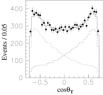
Figure 6: The $\cos\theta_{T}$ distribution observed at SLD (points), with the Monte Carlo prediction of the distributions for $b$ quarks (dashed), $\bar{b}$ quarks (dotted) and their sum (solid) overlayed.

The new measurements by the SLD collaboration [34, 35, 36] provide another example of the power of clean tagging and $b$ purity. While their sample of $Z^{0}$ decays is 20 times smaller than the individual LEP experiments, the $\Delta m_{d}$ sensitivity of an individual measurement is within a factor of two of individual LEP measurements. SLD takes advantage of the polarized beams at SLC, which produce a forward-backward asymmetry

$$\tilde{A}_{FB}=2A_{b}\frac{A_{e}+P_{e}}{1+A_{e}P_{e}}\frac{cos\theta_{T}}{1+\cos^{2}\theta_{T}},$$ (17)

in $Z^{0}\to b\bar{b}$ decays, where $A_{e}=0.155$ and $A_{b}=0.94$ specify the parity violation at the $Ze^{+}e^{-}$ and $Zb\bar{b}$ vertices, respectively, $P_{e}$ is the beam polarization, and $\theta_{T}$ is the angle between the thrust axis and the electron beam direction. The observed thrust angle distribution, with the expected asymmetric $b$ and $\bar{b}$ distributions superimposed, is shown in Figure 6. By combining the $\cos\theta_{T}$ information with other tag methods, SLD has increased the purity of their production flavor tag.

SLD has also boosted its $b$-quark purity to 93% in samples with inclusively reconstructed secondary vertices by requiring the mass $M$ and the transverse momentum $P_{T}$ of the vertex to satisfy

$$M_{P_{T}}=\sqrt{M^{2}+P_{T}^{2}}+\left|P_{T}\right|>2\,\,{\rm GeV}.$$ (18)

The decaying hadron’s mass must be at least $M_{P_{T}}$ to produce a vertex with the observed mass and $P_{T}$. They have also increased the $B^{0}$ purity of their samples by examining the total vertex charge. Use of these techniques has made these first SLD measurements competitive, with more data still to come.

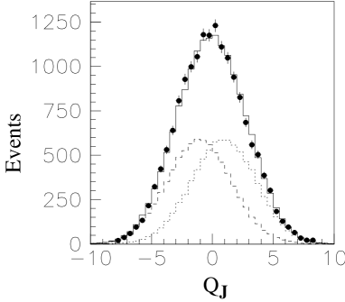
Figure 7: The jet charge $Q_{J}^{\rm\scriptsize opp}$ distribution observed at SLD (points), with the Monte Carlo prediction of the distributions for $b$ quarks (dashed), $\bar{b}$ quarks (dotted) and their sum (solid) overlayed.

Most production flavor tags rely primarily on the fact that the quarks are produced in $b\bar{b}$ pairs, and tag with variables sensitive to the $b$ quark flavor in the hemisphere (or jet) opposite that of the decaying $B$ candidate. Other production tags are based on fragmentation particles in the same hemisphere as the decaying $B$, which retain some information about the initial $b$ quark charge. A summary of the production tags follows:

• The jet charge is a weighted sum over the charges of the $n_{J}$ tracks within a hemisphere: $Q_{J}\sim\sum_{i=1}^{n_{J}}q_{i}|\vec{p}_{i}\cdot\hat{e}|^{\kappa}$, where $q_{i}$ and $\vec{p}_{i}$ are the charge and momentum of track $i$, and $\hat{e}$ is an estimate of the jet direction. For the jet charge $Q_{J}^{\rm\scriptsize opp}$ of the opposite hemisphere, the weight $\kappa$ is chosen near $0.5$ for ALEPH, DELPHI and SLD, and at 1 for OPAL. This tends to weight the charge of $B$ decay products most heavily (wanted when there is a charged $B$ in the opposite hemisphere), while still retaining the information content of the fragmentation particles (needed when the opposite $B$ is neutral). The SLD $Q_{J}^{\rm\scriptsize opp}$ distribution is shown in Figure 7. For the jet charge $Q_{J}^{\rm\scriptsize same}$ of the hemisphere containing the decaying $B$, experiments take $\kappa=0$. Neutral $B$’s contribute zero net charge, so the sum reduces to a sum of the fragmentation particles and the production tag is not biased by the decay flavor. Some analyses use $Q_{J}=Q_{J}^{\rm\scriptsize opp}-\alpha Q_{J}^{\rm\scriptsize same}$, with a weight $\alpha$ optimized with Monte Carlo. Jet charge tagging purities are on the order of 65% to 70%.

• A lepton in the opposite jet with large $p_{t}$ relative to the jet axis tags the charge of the $b$ quark. Such leptons preferentially select $B$ mesons, enhancing sample purity.

• A candidate leading fragmentation particle is chosen based on momentum and direction to the $B$. For $B^{0}$ candidates, a $\pi^{+}$ is favored as the leading fragmentation particle, since the $\bar{b}$ quark “pairs” with the $d$-quark from a $d\bar{d}$ pair, with the $\bar{d}$ left to form a $\pi^{+}$. The same sign correlation is expected from $B^{**}$ decays. CDF [37] finds an excess of correct-sign tags over wrong-sign tags of about 22% in their sample. For $B_{s}$ mixing, the sign of the leading charged kaon in the fragmentation products tags the production flavor.

• As discussed above, SLD can use their forward backward asymmetry to enhance tagging purity. The measurement is independent of the $Q_{J}$ measurement, and they combine the two to obtain a production tagging purity of 84%.

Some analyses use a combination of several tags to determine the production flavor.

The $b$ quark flavor at the time of decay is determined by examining the charge of one or more of the decay products. The various decay tags include

• As above.

• $D^{*\pm}$ mesons are fully reconstructed and their charge used to tag the decay flavor.

• $D^{*\pm}X\ell^{-}\nu$ are partially reconstructed using the lepton and the slow charged pion ($\pi^{*}$) from the $D^{*\pm}$ decay.

• The sign of charged kaons from the decay chain $b\to c\to s$ tags the decay flavor.

• For neutral $B$ decays involving a $D^{\pm}$, the $D^{\pm}$ lifetime induces a charge separation between the $B$ decay vertex and the $D^{\pm}$ vertex. The sign of the dipole moment evaluated along $B$ flight direction tags the production flavor.

Again, the decay tag sometimes consists of a combination of several methods.

Figure 8: The mixed event fraction $R$ as a function of proper time for the OPAL $D^{*\pm}+\ell/Q_{J}$ analysis. The curve is the result of the fit.

Based on the production and decay flavor tags, the fraction of mixed events as a function of proper time is determined. The resulting distribution for the OPAL $D^{*\pm}+\ell/Q_{J}$ analysis [38] is shown in Figure 8. The first half cycle, with the statistical precision degraded by the end, is clearly visible. These distributions are fit to a signal (mixing) term governed by ${\cal P}_{m}(t)$ (Eq. 9) convoluted with a resolution function, plus background terms for non-$B^{0}$ contributions and mistagging. The $\Delta m_{d}$ results from the time dependent measurements of ALEPH [32], DELPHI [30], L3 [31], OPAL [33, 38, 39], SLD [34, 35, 36] and CDF [37, 40] at the time of the conference are summarized in Figure 9. The results based on measurements of $\chi_{d}$ at the $\Upsilon(4S)$ [41, 42] and the averages for each experiment are also shown. The world average is $\Delta m_{d}=0.466\pm 0.012\pm 0.013\,\hbar\,{\rm ps}^{-1}$. The precision is under 4%.

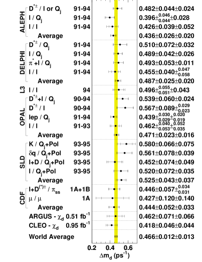
Figure 9: Summary of $\Delta m_{d}$ measurements. The grey band indicates the world average. Method and data sample are listed at left, the results at right.

In the averaging, correlated systematic errors must be addressed. Ignoring all correlations is unrealistic; assuming that similar techniques have fully correlated systematics will probably overestimate the correlations, and will miss correlations that exist between the other measurements. For each technique, only a subset of the errors categorized by all experiments has been considered in the individual measurements. To compensate for this somewhat, I have made coarse categories of correlated categories:

• Lifetimes of $B^{0}$, $B^{+}$, $B_{s}$, and $b$ baryons. Contributions from different lifetimes within a $\Delta m_{d}$ measurement are added in quadrature and this total error is taken as the correlated error when comparing measurements.

• Similarly for $D$ lifetimes.

• The fraction of $b$ baryons produced in $b\bar{b}$ hadronization.

• The fraction of $B_{s}$ produced in $b\bar{b}$ hadronization.

• The $c\bar{c}$ fraction of $Z^{0}$ decays.

• Similarly for the total fraction of $usd$.

• The average $B$ momentum at the $Z^{0}$, ie., $<p_{B}>/E_{\rm\scriptsize beam}\sim 70\%$ at LEP.

• For leptons from $b$, the fraction $f_{bc}$ from the cascade $b\to c\to l$.

• In the cascade $b\to c\to l$, the fraction from $B_{d}$ and from charged $B$’s.

• Uncertainties from the fraction of $D^{**}$’s in $B$ decays, and for analyses that reconstruct $D^{*}$’s, the fraction contributed by $B^{+}$.

• $\Delta m_{s}$.

• Uncertainty in the charged and neutral $B$ production fraction in the $\chi_{d}$ measurements at the $\Upsilon(4S)$.

The total systematic for each measurement in each category is shown in Table 1. If an experiment has already combined some or all of their measurements, I have listed the systematic for that combined measurement.

Were the correlations ignored, the systematic error would have dropped to $0.009\,\hbar\,{\rm ps}^{-1}$. Even though the correlated errors considered are relatively minor, they increase the error by 50%!. A LEP group has formed to perform a more systematic averaging of $\Delta m_{d}$. These results indicate that for individual measurements, a systematic uncertainty can be neglected only if small on the scale of the statistical error of that world average, not if it is small only on the scale of the uncertainty in that particular measurement.

Table 1: The correlated systematic on $\Delta m_{d}$ in each of the 12 categories for the different experiments (or measurements). The total systematic is shown for comparison. The units are $10^{-3}\,\hbar\,{\rm ps}^{-1}$.

Experiment	Method	Total	Systematic in Correlated Category
		systematic	1	2	3	4	5	6	7	8	9	10	11	12
ALEPH	$D^{\pm}$/$\ell$ or $Q_{J}$	24	3	2	0	0	0	0	7	0	0	18	0	0
ALEPH	$\ell$/$Q_{J}$,$\ell$/$\ell$	30	16	0	5	5	0	0	0	21	3	0	4	0
DELPHI	Comb.	20	6	0	5	9	1	0	4	10	3	6	0	0
L3	$\ell$/$\ell$	43	4	0	17	37	1	1	15	0	0	0	1	0
OPAL	$D^{\pm}$+$\ell$/$Q_{J}$	24	7	0	0	0	0	0	0	0	0	19	0	0
OPAL	$D^{\pm}$/$\ell$	${}^{+29}_{-23}$	7	0	0	8	14	0	0	0	0	9	0	0
OPAL	$\ell$/$Q_{J}$	19	5	0	5	4	0	0	0	2	0	0	0	0
OPAL	$\ell$/$\ell$)	${}^{+52}_{-35}$	22	0	12	28	0	0	0	0	11	8	6	0
SLD	Comb.	37	9	7	10	10	0	0	10	5	3	2	4	0
CDF	$D^{\pm}$+$\ell$/$\pi_{ss}$	${}^{+34}_{-31}$	3	0	0	0	0	0	0	0	0	29	0	0
CDF	$\mu/\mu$	140	0	0	0	0	0	0	0	0	113	0	0	0
ARGUS	$\chi_{d}$	66	15	0	0	0	0	0	0	0	0	0	0	20
CLEO	$\chi_{d}$	44	13	0	0	0	0	0	0	0	0	0	0	20

2.3.2 $B_{s}-\bar{B}_{s}$ mixing

Over the past year there have been two significant developments in the effort to determine $\Delta m_{s}$. The oscillations have not yet been observed, but the lower limit on $\Delta m_{s}$ has improved significantly.

First, the analyses themselves have improved. The older analysis techniques were based on the same $\ell/\ell$ and $\ell/Q_{J}$ samples used in the $\Delta m_{d}$ analyses. While these inclusive samples have high statistics, the $B_{s}$ content was low (10%) and the $\Delta m_{s}$ bounds were sensitive to the fraction $f_{B_{s}}$ of $b$ quarks that hadronize to form a $B_{s}$. The $B_{s}$ samples have been enriched by using reconstructed $D_{s}$ or $\phi$ mesons in conjunction with a high $p_{t}$ lepton (or high momentum hadron) to tag the decay flavor. These analyses have a $B_{s}$ content ranging from 25% up to as high as 60%. In addition, because of the exclusively reconstructed final state, the proper time resolution has improved, which is crucial for observing the rapid oscillation of the $B_{s}$ system.

The second breakthrough is a new technique for extracting the lower $\Delta m_{s}$ limit. Previously, the limits were determined from the likelihood difference curves obtained from fitting to the mixed event fraction: $-\Delta\log{\cal L}(\Delta m_{s})=\log{\cal L}(\Delta m_{s}^{\rm\scriptsize max})-\log{\cal L}(\Delta m_{s})$, where $\Delta m_{s}^{\rm\scriptsize max}$ is the mass difference that maximizes the likelihood. If the oscillation period is small relative to the proper time resolution, the value of $\Delta m_{s}^{\rm\scriptsize max}$ tends to be biased [47] towards a frequency at which the true amplitude is comparable to the statistical noise, so the likelihood function must be “calibrated” to determine the correct 95% C.L. limit. This has been done for each measurement by studying many toy experiments generated from a fast MC to determine the likelihood change that encompasses 95% of the experiments at a given $\Delta m_{s}$.

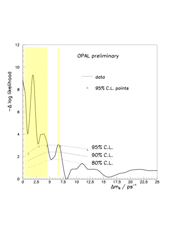
Figure 10: The OPAL combined likelihood curve (solid) as a function of $\Delta m_{s}$ for their three $\Delta m_{s}$ analyses, and the Monte Carlo calibration curves for the confidence levels 95%,90% and 80%. The shaded regions indicate $\Delta m_{s}$ values excluded at 95% C.L..

Combining the $-\Delta\log{\cal L}$ curves from different measurements is difficult. The resolutions involved are non-Gaussian; the systematics are correlated between measurements; the curve from each measurement has local minima and maxima. Under these conditions, there is not a well-defined procedure for combining the different curves. Furthermore, the combined likelihood itself must be recalibrated before a lower limit can be obtained, which offers a severe impediment to the combination of results from different experiments. The OPAL collaboration has, however, done a beautiful job of combining [48] their three $\Delta m_{s}$ likelihood curves [38, 39, 48]. The resulting likelihood and MC calibration are shown in Figure 10.

An alternative technique for extracting $\Delta m_{s}$ has been developed [47, 50] for ALEPH by Moser and Roussarie. Rather than extracting a likelihood as a function of $\Delta m_{s}$, their procedure, the “amplitude method”, is essentially a Fourier-transform. In their fit function, they replace the mixed decay probability ${\cal P}_{m}$ of Eq. 9 with

$${\cal P}_{m}(t)=\frac{\Gamma}{2}e^{-\Gamma t}[1-A\cos(\nu t)].$$ (19)

The frequency $\nu$ is fixed, and one fits for the amplitude $A$ of that frequency component in the data. For frequencies $\nu$ far from the true value of $\Delta m_{s}$, the amplitude should be zero. As $\nu$ approaches $\Delta m_{s}$, $A\to 1$. The distribution of $A$ should be the Fourier-transform of (9), a Breit-Wigner with a width of $2/\tau_{B_{s}}\approx 1.3\,{\rm ps}^{-1}$. One scans over values of $\nu$, fitting for the frequency components $A(\nu)$. $\Delta m_{s}$ is excluded from frequency ranges over which the amplitudes are less than one at the 95% C.L., ie. where $A(\nu)+1.645\sigma_{A}(\nu)<1$. Both ALEPH [49] and DELPHI [43] have evaluated their $\Delta m_{s}$ limits using this technique.

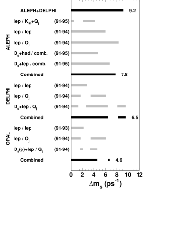
Figure 11: The $\Delta m_{s}$ regions excluded at the 95% C.L. by the ALEPH, DELPHI and OPAL measurements (grey bands). Also shown are the excluded regions from the combined measurements (black bands) of ALEPH+DELPHI (amplitude method – a.m.), ALEPH (a.m.), DELPHI (a.m.) and OPAL ($-\Delta\log{\cal L}$), with the 95% lower $\Delta m_{s}$ limit in each case.

The results of the ALEPH, DELPHI and OPAL $\Delta m_{s}$ analyses are summarized in Figure 11. The amplitudes extracted from different measurements are simple to combine — $A(\nu)$ at a given frequency is a physical measurement with a well-defined uncertainty. ALEPH and DELPHI have combined all of their measurements in this fashion to obtain improved lower limits. Combining $A(\nu)$ from both experiments yields the data shown in Figure 12, from which the lower bound $\Delta m_{s}>9.2\,\hbar\,{\rm ps}^{-1}$ is obtained. The amplitude error provides an estimate of the sensitivity to $\Delta m_{s}$. For the combined results the estimated sensitivity is $10.1\,\hbar\,{\rm ps}^{-1}$, larger than the lower bound.

Figure 12: $A(\Delta m_{s})$ versus $\Delta m_{s}$ for the combined ALEPH and DELPHI measurements (solid circles). The solid curve represents $A+1.645\sigma_{A}$; its intersection with 1 (open circle) determines the 95% C.L. lower bound. The dotted curve shows $1.645\sigma_{A}$; its intersection with 1 (open square) indicates the $\Delta m_{s}$ sensitivity of the combined analysis

2.4 Summary of $|V_{td}|$ and $|V_{ts}|$

Figure 13: The one standard deviation bounds (dotted curves) for $|V_{td}/V_{ts}|$ versus $f_{B_{d}}\sqrt{B_{B_{d}}}$ from a recent UT-analysis of Ali and London [51], assuming $V_{ts}=V_{cb}$, which is valid within the Wolfenstein approximation. The solid horizontal line is the upper limit on $|V_{td}/V_{ts}|$ from the $\Delta m_{d}$ and $\Delta m_{s}$ results presented here combined with the 95% C.L. upper limit on $\xi=1.15\pm 0.05$. The dashed line corresponds $\xi=1.3$.

While we now have a precise determination of the mass difference $\Delta m_{d}=0.466\pm 0.018\,\hbar\,{\rm ps}^{-1}$, uncertainty in $f_{B_{d}}\sqrt{B_{B_{d}}}$ currently limits the precision in the value of $|V_{td}|$ that can be extracted from this measurement. Combining this result with (12) and (14), one obtains a range for $|V_{td}|$ of 0.005 to 0.015. However, the 95% C.L. limit $\Delta m_{s}>9.2\,\hbar\,{\rm ps}^{-1}$, combined with this measurement of $\Delta m_{d}$, begins to prove interesting. If we also take a 95% C.L. upper limit on $\xi$ (c.f. (15)) based on $\xi=1.15\pm 0.05$, then Eq. 16 implies $|V_{td}/V_{ts}|<0.29$. This begins to restrict the allowed range of $f_{B_{d}}\sqrt{B_{B_{d}}}$ in UT analyses, as Figure 13 suggests. Even with $\xi$ as high as 1.3, a 95% C.L. limit of $|V_{td}/V_{ts}|<0.30$ is still constraining. SLD and CDF expect to limit $\Delta m_{s}$ with similar sensitivity.

The limits on the rare decay $K^{+}\to\pi^{+}\nu\bar{\nu}$ constrain $V_{td}$ at the ${\cal O}(0.1)$ level only. Data being taken now will significantly improve this limit. Comparison of rare $B$ processes $B\to\rho\gamma/B\to K^{*}\gamma$ yields a limit on $|V_{td}/V_{ts}|$ in the range $0.45-0.6$, depending upon the assumptions made and models used in the extraction of the limit. This is not far from the limit obtained from $\Delta m_{s}$ studies, and there is more data available at CLEO for measuring this ratio. In the long run, both methods should provide valuable information for $V_{td}$, unitary triangle analyses, and the quest for new physics.

3 Determining $|V_{cb}|$

Improving the precision on $|V_{cb}|$ remains a very important goal. $|V_{cb}|$ determines the Wolfenstein parameter $A$ in UT analyses. Since $A$ appears raised to large powers in some of the theoretical constraints, the effect of any uncertainty is magnified. Burchat and Richman [52] point out that even though $|V_{cb}|$ is already known quite precisely, its contribution to the uncertainty in the constraints on $\rho$ and $\eta$ from the $CP$-violating parameter $\varepsilon$ in $K_{L}\to\pi\pi$ decay, relative to the constraints from the $B$ system, rivals the contribution from the nonperturbative correction $B_{K}$.

There are two complementary approaches to the precise determination of $|V_{cb}|$: inclusive measurement of the total semileptonic $b\to c$ branching fraction, and measurement of the $B\to D^{*}\ell\nu$ hadronic form factor ${\cal F}$ at the zero recoil point. Since some of the key inputs that are used to control the theoretical uncertainties remain to be verified experimentally, agreement between the two methods provides a powerful consistency check.

3.1 Inclusive measurements

Extraction of $|V_{cb}|$ through the inclusive measurement of the total $B$ (or $b$) semileptonic branching fraction has the advantage of great statistical power. The semileptonic partial width can be written as

$$\Gamma=\Gamma_{0}\left\{1-a_{1}(\frac{m_{b}^{2}}{m_{c}^{2}})\frac{\alpha_{s}}{\pi}+\frac{a_{\rm np}}{m_{b}^{2}}+{\cal O}(\alpha_{s}^{2},\frac{\alpha_{s}}{m_{b}^{2}},\frac{1}{m_{b}^{3}})\right\},$$ (20)

where the $\Gamma_{0}$ is the tree level rate

$$\Gamma_{0}=\frac{G_{F}^{2}m_{b}^{5}}{192\pi^{3}}|V_{cb}|^{2}z_{0}(\frac{m_{b}^{2}}{m_{c}^{2}}),$$ (21)

$a_{1}$ is the first order perturbative QCD correction, $a_{\rm np}$ is the nonperturbative correction, and $z_{0}$ is a phase space factor. The exact form for these terms can be found elsewhere [53, 54, 55]. The nonperturbative correction is small and known to about 10% of itself, contributing little to the overall uncertainty in the predicted rate. One might expect uncertainty in the $b$ quark mass to introduce large uncertainties in the total rate via the $m_{b}^{5}$ dependence. Recent calculations by Shifman et al. [56] and Ball et al. [57] of $\Gamma/|V_{cb}|^{2}=41.3\pm 4\,{\rm ps}^{-1}$ and $43.2\pm 4.2\,{\rm ps}^{-1}$, respectively, have rather small (10%) uncertainties, though. Two factors appear to mollify the $b$ mass uncertainty. As Uraltsev [64] discusses, the variation of $a_{1}$ with $m_{b}$ tends to cancel the variation of the tree-level rate $\Gamma_{0}$. A significant reduction also comes [56] from constraining the mass difference $m_{b}-m_{c}$ to the heavy quark expansion prediction

$$m_{b}-m_{c}=\bar{M}_{B}-\bar{M}_{D}+\frac{\mu_{\pi}^{2}}{2}(\frac{1}{m_{c}}-\frac{1}{m_{b}})+\cdots,$$ (22)

where the “spin-averaged mass” $\bar{M}_{H}=\frac{1}{4}(M_{H}+3M^{*}_{H})$ and $\mu_{\pi}^{2}$ parameterizes the $b$ quark kinetic energy within the hadron. An agressive uncertainty, on the order of 50 MeV, was adopted for $m_{b}$ by these authors. The validity of these constraints have yet to be tested experimentally. For this review, I will average the two calculations and use the 10% uncertainty estimate, $\Gamma/|V_{cb}|^{2}=(42.3\pm 4.2)\,{\rm ps}^{-1}$.

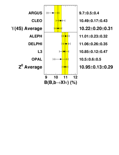
Figure 14: The inclusive branching ratios ${\cal B}(B\to X\ell\nu)$ and ${\cal B}(b\to X\ell\nu)$ measured at the $\Upsilon(4S)$ and the $Z^{0}$, respectively. The grey bands indicate the averages.

Experimentally, the discrepancies between semileptonic rates for the $B$ meson, measured [58, 42, 59] at the $\Upsilon(4S)$, and the $b$ quark, measured [60, 61, 62, 63] at the $Z^{0}$, have decreased. For the $\Upsilon(4S)$ the dilepton measurements are quoted, as preferred by those experiments, since while statistical uncertainties are larger than in the single lepton measurements, the model dependence is much smaller. I quote the lifetime-tagged ALEPH result for the same reason. Figure 14 summarizes the current situation. The lifetime-tagged ALEPH analysis and the new L3 results in particular have helped to alleviate the discrepancy.

Taken at face value, the branching ratios agree within 1.5 standard deviations. However, given the short $b$ baryon lifetimes, one would actually expect the LEP value to be lower than that measured at the $\Upsilon(4S)$, and the real discrepancy is more severe.

It should be noted that these measurements are the combination of the 2 processes $b\to c\ell\nu$ and $b\to u\ell\nu$. Rosner estimates [65] the $b\to u$ fraction to be $(1.85{\rm\ to\ }2.44)|V_{ub}/V_{cb}|^{2}$, or about $(1.5\pm 1.0)$%. While this seems small, it is of the same order as the experimental statistical uncertainties and therefore should be corrected for. After correction, the average $B$ meson and $b$ quark charmed semileptonic branching fractions are $(10.07\pm 0.38)$% and $(10.79\pm 0.33)$%, respectively. The statistical, systematic and $|V_{ub}|$ correction uncertainties have been combined in quadrature.

These measurements, the average lifetimes [66] at the $\Upsilon(4S)$ and $Z^{0}$ of $<\!\tau_{B}\!>\,=1.59\pm 0.04$ ps and $<\tau_{b}>=1.55\pm 0.02$ ps, and the rate prediction combine to give

$\Upsilon(4S)$ : $|V_{cb}|=\,$	$(38.7\pm 0.9\pm 1.9)\times 10^{-3}$
$Z^{0}$ : $|V_{cb}|=\,$	$(40.6\pm 0.7\pm 2.0)\times 10^{-3}$

3.2 $B\to D^{*}\ell\nu$

Measurement of the $B\to D^{*}\ell\nu$ differential decay rate at the zero recoil point currently provides the determination of $|V_{cb}|$ with the least theoretical uncertainty. The experimental techniques have been reviewed in some detail [67, 68, 69, 70]. The measurements are reviewed briefly here, with the focus on an improved averaging procedure that accounts for the correlation between the extracted form factor slopes and $|V_{cb}|$.

The differential decay rate for $B\to D^{*}\ell\nu$ is given by

$$\frac{d\Gamma}{dw}=\frac{G_{F}^{2}}{48\pi^{3}}\kappa(m_{B},m_{D},w)|V_{cb}|^{2}{\cal F}^{2}(w),$$ (23)

where $w=v_{B}\cdot v_{D^{*}}=(m_{B}^{2}+m_{D^{*}}^{2}-q^{2})/2m_{B}m_{D^{*}}$, and is the boost of the $D^{*}$ in the $B$ rest frame, $q^{2}$ is the four-momentum transfer to the leptonic system, and $\kappa$ is a known function. In general, the form factor ${\cal F}(w)$ cannot be calculated in a model-independent fashion.

At the zero-recoil point $w=1$, however, heavy quark effective theory (HQET) allows calculation of ${\cal F}(1)$ with controllable theoretical uncertainties. HQET and experimental tests are discussed in more detail in the talks of Richman [4] and Martinelli [5] and, for example, in various reviews by Neubert [71, 72]. HQET predicts that ${\cal F}(1)\to 1$ for transitions between heavy quarks, with corrections at the level of $1/m_{q}$ or smaller. At this zero recoil point, the heavy quark changes flavor without perturbing its color field, so there is little suppression of the decay rate at that point.

Experimentally, then, one must determine the form factor at $w=1$. Unfortunately, the differential decay rate rate vanishes at $w=1$, so ${\cal F}(w)$ must be measured nearby and extrapolated to $w=1$. Since the true function ${\cal F}(w)$ is unknown, it is expanded around the zero recoil point,

$${\cal F}(w)={\cal F}(1)[1-\hat{\rho}^{2}(w-1)+\hat{c}(w-1)^{2}+\cdots].$$ (24)

While experiments have attempted to extract both the slope and the curvature, they are not yet sufficiently sensitive to constrain $\hat{c}$, and therefore quote results for strictly linear fits. A positive curvature must exist, but only a small bias is introduced from the linear restriction because the physically allowed range for $w$, from 1 to 1.5, is rather small. The bias will be estimated later.

The decay $B\to D^{*}\ell\nu$ is favored over $D\ell\nu$ for several reasons. First of all, as Luke [73] noted, the ${\cal O}(\Lambda_{\rm\scriptsize QCD}/m_{b})$ corrections to ${\cal F}(1)$ vanish for $D^{*}\ell\nu$. The calculations for ${\cal F}(1)$ for $B\to D^{*}\ell\nu$ have also been much more thoroughly scrutinized. Experimentally, the $D^{*}\ell\nu$ mode has the largest branching fraction, and it is not helicity-suppressed near $w=1$, while $D\ell\nu$ is. Hence a more precise and reliable extrapolation to $w=1$ is possible for $D^{*}\ell\nu$.

Figure 15: Reconstructed mass difference for DELPHI inclusive $D^{0}$ $|V_{cb}|$ analysis. (a) Right sign $\ell^{\pm}\pi^{\mp}$ combinations in data (points), background MC (dashed histogram) and signal MC (open histogram). (b) Wrong sign $\ell^{\pm}\pi^{\pm}$ combinations. (c) Data after simulated background subtraction.

Most measurements [42, 74, 75, 76, 77] have used the decays $B^{0}\to D^{*-}\ell^{+}\nu$, $D^{*-}\to\pi^{-}\bar{D}^{0}$, explicitly reconstructing $\bar{D}^{0}\to K^{+}\pi^{-}(n\pi)$. DELPHI [76] has, in additional, inclusively reconstructed the $D^{0}$ meson, to obtain one of the most precise recent measurements of ${\cal F}(1)|V_{cb}|$. While their $D^{0}$ mass resolution of 700 MeV is quite broad, they do see a clear $D^{*}$ signal in the mass difference distribution $\Delta M=M_{D^{0}\pi}-M_{D^{0}}$ (Figure 15). CLEO [75] has used $B^{-}\to D^{*0}\ell^{-}\bar{\nu}$, $D^{*0}\to D^{0}\pi^{0}$ in addition to the neutral $B$ decays.

With an undetected neutrino in the final state, estimating $w$ is challenging. At the $\Upsilon(4S)$, the $B$ mesons are nearly at rest, so $w=E_{D^{*}}/M_{D^{*}}$ is an excellent approximation, yielding a $w$ resolution of about 4% of the total 1-1.5 range. At the $Z^{0}$, the $B$ energy is not known, but with the large boosts, $w$ can be estimated from the $B$ flight direction and missing energy constraints. The resulting $w$ resolutions at LEP are about 15% to 20% of the total range for the exclusive analyses, and about 20% to 40% for the DELPHI inclusive analysis. The reconstructed $w$ distributions are then fit using (23) to obtain ${\cal F}(1)|V_{cb}|^{2}$ and $\hat{\rho}$, properly accounting for the smearing of $w$.

The $\Upsilon(4S)$ and $Z^{0}$ measurements complement each other nicely. Because of the very soft $B$’s at the $\Upsilon(4S)$, the $w$ resolution is excellent and simple lepton momentum and kinematic requirements reduce $D^{**}$ backgrounds to about 5%. On the other hand, the low $B$ momentum means that the charged $\pi$’s from the $D^{*}$ decays are very soft near $w=1$, resulting in poor reconstruction efficiency where the information is most important for the extrapolation to $w=1$. Because of the large boost of the $B$’s at LEP, the $D^{*}$ reconstruction efficiency is good near $w=1$. The $w$ resolution, however, is much worse, and the $D^{**}$ backgrounds are severe – of order 15%. This is unfortunate, since we are now only beginning to obtain reliable information concerning $B$ decays to $D^{**}$.

Table 2: Results from fits to the observed $w$ distributions for $B\to D^{*}\ell\nu$. The parameters $\rho_{\rm\scriptsize stat}$ and $\rho_{\rm\scriptsize sys}$ are the statistical and systematic correlation coefficients between $F(1)|V_{cb}|/10^{-3}$ and $\hat{\rho}$. All intercepts have been scaled to a common set of branching ratios and lifetimes (see text). For the DELPHI-avg, the “statistical’ correlation coefficient listed is the total correlation coefficient for the averaged exclusive and inclusive results, excluding the small (0.04) common systematic. The results for $B\to D\ell\nu$ are also listed.

		$F(1)|V_{cb}|/10^{-3}$	$\hat{\rho}$	$\rho_{\rm\scriptsize stat}$	$\rho_{\rm\scriptsize sys}$
$D^{*}\ell\nu$	ALEPH	$31.0\pm 1.8\pm 2.0$	$0.29\pm 0.18\pm 0.12$	0.921	0.612
	DELPHI-incl	$36.4\pm 2.2\pm 2.6$	$0.74\pm 0.20\pm^{0.18}_{0.16}$	0.96	0.816
	DELPHI-excl	$35.2\pm 3.5\pm 3.0$	$0.77\pm 0.26\pm 0.10$	0.906	0.616
	DELPHI-avg	$36.5\pm 2.1\pm 2.2$	$0.78\pm 0.16\pm 0.10\pm 0.04$	0.869	0.0
	OPAL	$33.9\pm 2.9\pm 2.3$	$0.44\pm 0.24\pm 0.12$	0.95	0.577
	ARGUS	$39.0\pm 3.9\pm 2.8$	$1.17\pm 0.24\pm 0.06$	0.90	0.601
	CLEO	$35.1\pm 1.9\pm 1.8$	$0.84\pm 0.12\pm 0.08$	0.90	0.610
$D\ell\nu$	CLEO - $\nu$	$36.2\pm 5.7\pm 4.2$	$0.73\pm 0.24\pm 0.10$	0.940	0.725
	CLEO - kinem.	$32.7\pm 6.0\pm 5.3$	$0.52\pm 0.29\pm 0.10$	0.972	0.574
	ALEPH	$38.8\pm 6.7\pm 6.9$	$0.00\pm 0.49\pm 0.38$	0.986	0.953

The experimental results are summarized in Table 2. All results have been updated to the following common set of constants:

$R_{b}$ [74] :	$(22.09\pm 0.21)$%
${\cal B}(b\to B^{0})$ [66] :	$(37.8\pm 2.2)$%
$\tau_{B^{0}}$ [78] :	$(1.56\pm 0.05)$ ps
$\tau_{B^{+}}/\tau_{B^{0}}$ [78] :	$1.02\pm 0.04$
${\cal B}(D^{0}\to K^{-}\pi^{+})$ [4] :	$(3.88\pm 0.1)$%

The statistical correlation coefficients from the individual fits are quite large. (Note: ARGUS has not published its coefficients – I have assumed that they are similar to CLEO’s. OPAL did not list the systematic uncertainties on their slope, so $\rho_{\rm\scriptsize sys}$ is estimated to be similar to the other LEP coefficients.) If statistical fluctuations or systematic biases have resulted in a low slope in the fit, the intercept will be lowered as well. Hence the intercepts should not be averaged without regard to the slopes.

The one standard deviation error ellipses are shown for the five experiments in Figure 16. While the intercepts appear consistent, the measured slopes do not — they are consistent only at the 5% confidence level. Note that a precise measurement of the form factors by CLEO [79], for which backgrounds have been highly suppressed, implies that the average slope measured in these analyses should be $\hat{\rho}\approx 0.77\pm 0.22\pm 0.07$. An averaging of the slopes and the intercepts simulataneously with their correlations and also correlated systematic errors between experiments taken into account yields ${\cal F}(1)|V_{cb}|=0.0348\pm 0.0016$. The $\chi^{2}$ is 12.2 for 8 degrees of freedom. Since the errors in $|V_{cb}|$ should reflect the unsettling state of the slopes, I’ve chosen to adopt the Particle Data Group procedure and to scale the error by $\sqrt{12.2/8}$. The final result is then ${\cal F}(1)|V_{cb}|=0.0348\pm 0.0020$ The average slope, also with errors scaled, is $\hat{\rho}=0.75\pm 0.11$.

Figure 16: One standard deviation error ellipses for ${\cal F}(1)|V_{cb}|$ versus the form factor slope $\hat{\rho}^{2}$. The black cross-hatched ellipse is the average.

We must address the bias induced by the linear form factor parameterization in the fits. Patterson [67] and Stone [68] have evaluated the possible shifts in a variety of models, and find that corrections of up to $+4\%$ might be necessary. ALEPH [74] has fit using constraints on the curvature $\hat{c}$ versus $\hat{\rho}$ estimated [81]by Cabrini and Neubert. While their central value does not change, the statistical uncertainty increases by 4%. It seems that an additional uncertainty of 4% is appropriate for the linear bias. For an estimate of the bias, I used the Cabrini–Neubert relationship to find the curvature that would yield on average the slope observed in a linear fit. This procedure implies an average bias in the fits of -2.5%. After a $(2.5\pm^{4}_{2.5})$% correction, ${\cal F}(1)|V_{cb}|=(35.7\pm 2.1\pm^{1.4}_{0.9})\times 10^{-3}$, where the errors are the experimental uncertainty and the bias uncertainty, respectively.

To extract $|V_{cb}|$, we need a prediction for $F(1)=\eta_{A}(1+\delta_{1/m^{2}})$, where $\eta_{A}$ is the perturbative QCD correction, and $\delta_{1/m^{2}}$ incorporates the $1/m_{b}^{2}$ and $1/m_{c}^{2}$ corrections. Recently, Czarnecki [80] has completed a complete two-loop calculation of the perturbative correction, finding $\eta_{A}=0.960\pm 0.007$. Neubert has summarized [71] the work done by various authors [56, 82, 83, 84] for the $1/m^{2}$ correction, finding $\delta_{1/m^{2}}=(-5.5\pm 2.5)$%. The predictions of HQET are now just beginning to be tested, for example through the measurement of the individual form factors in $B\to D^{*}\ell\nu$ decays [79].

The total correction is therefore ${\cal F}(1)=0.91\pm 0.03$, from which we obtain

$$|V_{cb}|=0.0391\pm 0.0027\pm 0.0013,$$ (25)

where the experimental and bias uncertainties have been combined in the first error, and the second error is the uncertainty in ${\cal F}(1)$.

3.3 $B\to D\ell\nu$

Both CLEO [85] and ALEPH [74] have results for similar form factor studies of the decay $B^{0}\to D^{-}\ell^{+}\nu$. CLEO has performed two analyses that have similar sensitivities and largely independent samples, one based on “neutrino-reconstruction” techniques that will be discussed below, and one based on the $D$–$\ell$ kinematics assuming the $B$ mesons produced at the $\Upsilon(4S)$ are at rest. The ALEPH analysis is similar to its $D^{*}\ell\nu$ analysis.

The results, after correcting to the standard branching ratios listed above, are also summarized in Table 2. The error ellipses for both experiments are shown in Figure 17. The CLEO results have been reaveraged with the slope and intercept correlations taken into account along with the common systematic uncertainties. The simultaneous average of the three slope and intercept measurements gives ${\cal F}(1)|V_{cb}|=(36.8\pm 4.0)\times 10^{-3}$ and $\hat{\rho}=0.58\pm 0.20$. For the intercept in particular, it is clear from Figure 17 that a naive average would have resulted in a very biased result — almost a full standard deviation lower than the results obtained here.

Figure 17: One standard deviation error ellipses for ${\cal F}(1)|V_{cb}|$ versus the form factor slope $\hat{\rho}^{2}$ for $B^{0}\to D^{-}\ell^{+}\nu$. The black cross-hatched ellipse is the average.

While the prediction of ${\cal F}(1)$ for $D\ell\nu$ has not received nearly the scrutiny as the $D^{*}\ell\nu$ prediction, a recent calculation predicts [81, 86] ${\cal F}(1)=0.98\pm 0.07$. Taking this calculation, and assuming the same bias from the linear form factor parameterization as in the $D^{*}\ell\nu$ case, we have $|V_{cb}|=0.0385\pm 0.0045\pm 0.0028$.

3.4 Summary

The $V_{cb}$ values obtained from inclusive measurements at the $\Upsilon(4S)$ and at LEP and from the exclusive $B\to D^{(*)}\ell\nu$ decays are shown in Figure 18. The level of agreement between the different inclusive and exclusive measurements is quite good. The theoretical uncertainties in the inclusive and exclusive measurements are quite different, so the agreement is certainly heartening, and suggests that, at least at the 5% level, the theoretical calculations are in reasonable control. However, given the broad range of estimates for the theoretical uncertainties [64, 71], and the infancy of the experimental checks of the theoretical inputs, it seems premature to average the results.

Figure 18: Summary of the $|V_{cb}|$ measurements.

4 Determining $V_{ub}$

Until recently, the sole evidence for $b\to u$ transitions has come from the observation [87, 88] of leptons with momenta in a range accessible to $b\to u\ell\nu$, yet high enough to be reached only rarely in the dominant $b\to c\ell\nu$ process. These studies have yielded the oft-quoted value $|V_{ub}/V_{cb}|=0.08\pm 0.02$. Model dependence dominates the uncertainty — the details of hadronization significantly affect this endpoint region, and the rate into this range cannot be calculated reliably.

Experimentally, the rate measurements themselves show significant variation within a single model. Patterson [89] has re-evaluated those analyses: the discrepancies appear to arise from the procedure used to extract $|V_{ub}/V_{cb}|$ from the observed $b\to u\ell\nu$ rate. This was accomplished using the measured rate for inclusive $b\to c\ell\nu$ decays with leptons in a moderately high momentum range, allowing $|V_{ub}/V_{cb}|$ to be obtained directly. The procedure relied on modeling of both $b\to u\ell\nu$ and $b\to c\ell\nu$. If instead the $B$ lifetime, now known quite precisely, is used to directly extract $|V_{ub}|$, the experimental discrepancies vanish. The new average is compatible with the standard $|V_{ub}/V_{cb}|$ value in use, and the resolution of this problem lends considerable confidence that the the experimental uncertainty is reasonable.

ALEPH has presented [90] first evidence for observation of semileptonic $b\to u$ transitions at LEP. The large $b\to c$ background must be understood at the 1% level for the reliable extraction of $|V_{ub}|$, which seems difficult given our incomplete knowledge of the charm semileptonic decays of $B$ hadrons.

Exclusive charmless semileptonic decays provide an alternate route to $|V_{ub}|$. The theoretical road is still rocky, since the form factors for the exclusive decays must be known both for the determination of detection efficiencies and for the rate predictions needed to extract $|V_{ub}|$. Because these are heavy$\to$light transitions, HQET cannot help as it did for $b\to c\ell\nu$, and we must live with model dependence for now. There is great activity in the calculation of form factors spanning a variety of models and techniques, and consistency among the different technique will help to lend some confidence in the $|V_{ub}|$ extraction.

CLEO [89, 91] has recently extracted $|V_{ub}|$ from the study of the $B\to\pi\ell\nu$ and $B\to\rho/\omega\ell\nu$ decays of both $B^{+}$ and $B^{0}$. To suppress the large backgrounds from the dominant $b\to c\ell\nu$ processes, they use the missing energy $E_{\rm\scriptsize miss}$ and momentum $\vec{P}_{\rm\scriptsize miss}$ in the entire event to infer information about the missing neutrino. Selection requirements — zero observed charge, identically one observed lepton, $M^{2}_{\rm\scriptsize miss}\equiv E_{\rm\scriptsize miss}^{2}-\vec{P}_{\rm\scriptsize miss}^{2}\sim m_{\nu}^{2}=0$ — suppress events in which $\vec{P}_{\rm\scriptsize miss}$ would misrepresent a true primary neutrino. They find resolutions on the neutrino momentum and direction of 110 MeV (roughly 5%) and $6^{\circ}$, respectively. They can then fully reconstruct signal candidates, examining $M_{m\ell\nu}\equiv(E_{\rm\scriptsize beam}^{2}-|\vec{p}_{m}+\vec{p}_{\ell}+\vec{p}_{\nu}|^{2})^{1/2}$, which should peak at the $B$ mass, and $\Delta E\equiv E_{m\ell\nu}-E_{\rm\scriptsize beam}$, which should peak at zero. They see clear evidence for a signal in both variables (Figure 19) in both the $\pi$ modes and the $\rho/\omega$ modes. CLEO extracts branching ratios and $|V_{ub}|$ from fits to data in the region $|\Delta E|<0.75$ GeV and $5.1075\leq M_{m\ell\nu}<5.2875$ GeV.

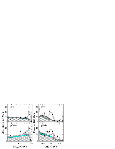
Figure 19: $M_{m\ell\nu}$ (left) and $\Delta E$ (right) distributions in the $\Delta E$ and $M_{m\ell\nu}$ signal bands, respectively. The data (points) have continuum and fake-lepton backgrounds subtracted. The coarse crosshatch, grey and unshaded components are $b\to cX$ background, feed-down background from other $B\to X_{u}\ell\nu$ decays, and signal, respectively. For the $\pi$ ($\rho/\omega$) modes, the fine crosshatch shows the signal mode cross-feed level $\rho/\omega\to\pi$ ($\pi\to\rho/\omega$) and the single hatch, $\pi\to\pi$ ($\rho/\omega\to\rho/\omega$) cross-feed.

CLEO has evaluated their experimental efficiencies using several models [92] that span a variety of calculation techniques. For the branching ratios, the model dependence is moderate because the efficiencies do not depend on the overall normalization of the form factors. CLEO can test the validity of a given model by comparing the measured ratio of branching fractions ${\cal B}(B\to\rho\ell\nu)/{\cal B}(B\to\pi\ell\nu)$, obtained with efficiencies determined from the model, to the ratio predicted by that model. The Körner and Schuler model was only consistent at the $0.5\%$ level, so it was excluded from any model averages. From the remaining models they obtained ${\cal B}(B^{0}\to\pi^{-}\ell^{+}\nu)=(1.8\pm 0.4\pm 0.3\pm 0.2)\times 10^{-4}$ and ${\cal B}(B^{0}\to\rho^{-}\ell^{+}\nu)=(2.5\pm 0.4^{+0.5}_{-0.7}\pm 0.5)\times 10^{-4}$, where the errors are statistical, systematic and the estimated model-dependence, respectively. The asymmetric error in the $\rho$ modes arises from the uncertainty in nonresonant $B\to\pi\pi\ell\nu$ background, which CLEO has limited by studying $\pi^{0}\pi^{0}\ell\nu$.

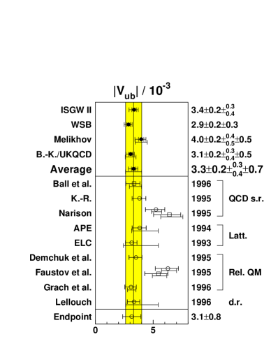
Figure 20: Values for $|V_{ub}|$ extracted from the exclusive CLEO measurements. Top section: Combined $\pi\ell\nu$ and $\rho\ell\nu$ results from models considered by CLEO. Middle section: Results based on CLEO model-averaged branching fractions and predictions from a sampling of other calculations based on QCD sum rules (QCD s.r.), lattice calculations (Latt.), relativistic quark models (rel. QM) and dispersion relations (d.r.). B.–K. refers to Burdman-Kambor; K.-R. refers to Khodjamirian–Rückl. Open circles (squares) are $\pi\ell\nu$ ($\rho\ell\nu$) results. Bottom section: Inclusive endpoint value. The points show the experimental errors. In the middle section, the estimated model dependence is included. An error bar underneath the data point indicates that model’s internal error. The grey band show CLEO’s estimated model dependence.

Extraction of $|V_{ub}|$ has greater model dependence because the absolute form factor normalization must be known. To combine the information from the $\pi$ and $\rho/\omega$ modes within a model, CLEO determines $|V_{ub}|$ by constraining the $\rho/\pi$ ratio to that predicted by the model. The resulting values are shown in the top of Figure 20, from which CLEO estimates $|V_{ub}|=(3.3\pm 0.2^{+0.3}_{-0.4}\pm 0.7)\times 10^{-3}$, where the errors are statistical, systematic, and estimated model dependence, respectively. Comparisons of a larger sampling of recent models [93], from which $|V_{ub}|$ has been extracted using the above branching fractions, are also shown. They generally agree with CLEO’s value, and suggest that the estimated model dependence is reasonable.

This new determination of $|V_{ub}|$ is in excellent agreement with the value obtained from the endpoint analysis, which bolsters confidence in the value used for the past few years. At the moment, it is not clear how to properly average these results, since the errors in both are dominated by theoretical uncertainties, uncertainties that in this case are correlated. The recent CLEO result is perhaps the most robust estimate to date.

5 CPLEAR – $CP$ and $CPT$

This year marks the close of data taking for the CPLEAR experiment. The many results of this beautiful experiment are summarized in these Proceedings by B. Pagels [94]. They have made many precise determinations of the $CP$-violating parameters in the neutral kaon system.

They have also made significant contributions to tests of $CPT$ conservation. There had been a long-standing two standard deviation discrepancy between the world average of $\phi_{+-}$ (the phase of the $CP$-violating parameter $\eta_{+-}$ in $K_{L}\to\pi^{+}\pi^{-}$ decay) and the “superweak phase” $\phi_{\rm\scriptsize sw}\equiv\tan^{-1}(\frac{2\Delta m}{\Gamma_{S}-\Gamma_{L}})$. Such a discrepancy would signal $CPT$ violation. Measurements by the FNAL E731 experiment [95] indicated that the problem lay with a high world average of the $K_{L}-K_{S}$ mass difference, $\Delta m$, with which $\phi_{+-}$ measurements are highly correlated. Among CPLEAR’s measurements are $\Delta m=(529.2\pm 1.8\pm 1.5)\times 10^{-7}\,\hbar\,{\rm s}^{-1}$, the most precise to date, and $\phi_{+-}=43.5^{\circ}\pm 0.5^{\circ}\pm 0.5^{\circ}\pm 0.4^{\circ}$. These measurements, along with other recent results [96], have confirmed this suggestion, and $CPT$ invariance is alive and well.

CPLEAR also has an indication of a $T$-violating asymmetry in $K$ semileptonic decay based on a fraction of their data, with the assumption that $CPT$ is conserved in the semileptonic decay amplitudes. Such an asymmetry is expected to accompany the known $CP$-violation in the neutral $K$ system. It will be exciting to see the results of this analysis from the full data sample.

6 Conclusion

In summary, the year has continued to benefit from the ingenuity brought to bear on weak quark mixing. We now know $\Delta m_{d}$ with outstanding precision. I look forward to improved calculations of $f_{B}$ and $B_{B}$ from the lattice and elsewhere. Limits on $\Delta m_{s}$ are beginning to provide useful constraints in unitary triangle analyses, and improved statistics for $\Delta m_{s}$ and for rare $B$ and $K$ decays hold great promise.

Values of $|V_{cb}|$ show excellent agreement in results obtained from inclusive and exclusive studies. Extraction of $|V_{cb}|$ from $D^{*}\ell\nu$ decays remains the most reliable determination. This method is currently statistically limited, and improvements should be seen soon. With the improving precision, proper handling of correlations is necessary, and understanding the experimental discrepancies in the form factor slopes is crucial. The unknown form factor curvatures could soon become a limiting factor in the precision.

Studies of $|V_{ub}|$ have entered a new era with the first determination from exclusive channels. These have bolstered our confidence in the inclusive determination, and provide a testing ground for exclusive models. This will help, in turn, reduce uncertainties in the inclusive determination.

Impressive as the precision of the measurements is becoming, the Standard Model remains unscathed. The next few years, as analyses of current experiments finish and as high luminosity $B$ experiments begin data-taking, hold the promise of much excitement.

References

References

- [1] N. Cabibbo, Phys. Rev. Lett. 10, 531 (1963).
- [2] M. Kobayashi and T. Maskawa, Prog. Theor. Phys. 49, 652 (1973)
- [3] L. Wolfenstein, Phys. Rev. Lett. 51, 1945 (1983).
- [4] J.R. Richman, these proceedings.
- [5] G. Martinelli, these proceedings.
- [6] A.J. Buras, these proceedings.
- [7] H. Albrecht et al. (ARGUS), Phys. Lett. B 192, 245 (1987).
- [8] D. Rein and L.M. Seghal, Phys. Rev. D 39, 3325 (1989).
- [9] J.S. Hagelin and L.S. Littenburg, Prog. Part. Nucl. Phys. 23, 1 (1989).
- [10] G.Buchalla and A.J. Buras, Nucl. Phys. B 412, 106 (1994).
- [11] S. Adler et al. (BNL E787), Phys. Rev. Lett. 76, 1421 (1996).
- [12] A. Khodjamirian, G. Stoll and D. Wyler Phys. Lett. B 358, 129 (1995)
- [13] A. Ali and V.M. Braun Phys. Lett. B 359, 223 (1995)
- [14] A. Ali, Proceedings of the XXXth Rencontres de Moriond “Electroweak Interactions and Unified Theories”, Moriond, France, March, 1995.
- [15] A. Ali, V.M. Braun, and H. Simma, Z. Phys. C 63, 437 (1994)
- [16] S. Narison, Phys. Lett. B 327, 354 (1994)
- [17] J.M. Soares, Z. Phys. C 63, 437 (1994)
- [18] S. Anderson et al. (CLEO), CLEO-CONF-96-06, ICHEP96 pa05-96, July, 1996.
- [19] I.I. Bigi, V.A. Khoze, N.G. Uraltsev, A.I. Sanda, in Violation, C. Jarlskog, ed., World Scientific, Singapore, 1989.
- [20] A.J. Buras, W. Slominski and H. Steger, Nucl. Phys. B 245, 369 (1984).
- [21] T. Inami and C.S. Lim, Prog. Theor. Phys. 65, 297 (1981).
- [22] A.J. Buras, M. Jamin and P.H. Weisz, Nucl. Phys. B 347, 491 (1990).
- [23] A.J. Buras, Proceedings of ’Beauty 95’, Oxford, England, July, 1995, Nucl. Instrum. Methods A 368, 1 (1995)
- [24] P. Tipton, these proceedings.
- [25] J. Flynn, these proceedings.
- [26] A.J. Buras, these proceedings and references therein.
- [27] S. Narison, Phys. Lett. B 322, 247 (1994).
- [28] S. Narison and A. Pivovarov, Phys. Lett. B 327, 341 (1994).
- [29] S.L. Wu, Talk at the /it 17th International Symposium on Lepton-Photon Interactions at High Energies, Beijing, China, Aug 1995, CERN-PPE-96-082, June, 1996.
- [30] P. Checchia et al. (DELPHI), DELPHI 96-87 CONF 016, ICHEP96 pa01-038, June, 1996, and references therein.
- [31] M. Acciarri et al. (L3), Phys. Lett. B 383, 487 (1996).
- [32] D. Buskulic et al. (ALEPH), ICHEP96 pa05-055, July, 1996, and references therein.
- [33] R. Akers et al. (OPAL), Z. Phys. C 66, 555 (1995)
- [34] K. Abe et al. (SLD), SLAC-PUB-7228, ICHEP96 pa08-026A, July, 1996.
- [35] K. Abe et al. (SLD), SLAC-PUB-7229, ICHEP96 pa08-026B, July, 1996.
- [36] K. Abe et al. (SLD), SLAC-PUB-7230, ICHEP96 pa08-027/28, July, 1996.
- [37] F. Abe et al. (CDF), FERMILAB-CONF-96/175-E, ICHEP96 pa08-032, July, 1996.
- [38] G. Alexander et al. (OPAL), CERN-PPE/96-074, June, 1996. Submitted to Z. Phys. C.
- [39] R. Akers et al. (OPAL), OPAL-PN196, August, 1995. Submitted to Lepton-Photon Symposium, Beijing, August, 1995.
- [40] F. Abe et al. (CDF), FERMILAB-CONF-95-231-E, July, 1995. Submitted to Lepton-Photon Symposium, Beijing, August, 1995.
- [41] J. Bartelt et al. (CLEO), Phys. Rev. Lett. 71, 1680 (1993).
- [42] H. Albrecht et al. (ARGUS), DESY-96-015, January, 1996, and references therein.
- [43] A. Borgland et al. (DELPHI), DELPHI 96-88 CONF 017, ICHEP96 pa01-039, June, 1996, and references therein.
- [44] R. Akers et al. (OPAL), OPAL-PN199, ICHEP96 pa08-014, December, 1995.
- [45] D. Buskulic et al. (ALEPH), Phys. Lett. B 377, 205 (1996).
- [46] D. Buskulic et al. (ALEPH), ICHEP96, pa05-054, July, 1996.
- [47] H.-G. Moser and A. Roussarie, /it Mathematical Methods for Oscillation Analyses, June, 1996. Submitted to Nucl. Instrum. Methods A.
- [48] R. Akers et al. (OPAL), OPAL-PN210, ICHEP96 pa08-010, March, 1996.
- [49] D. Buskulic et al. (ALEPH), ICHEP96, pa08-020, July, 1996, and references therein.
- [50] D. Buskulic et al. (ALEPH), EPS0410, Contributed to International Europhysics Conference on High Energy Physics, Brussels, Belgium, 1995.
- [51] A. Ali and D. London, DESY-96-140, July 1996.
- [52] P. Burchat and J. Richman, Rev. Mod. Phys. 67, 893 (1995)
- [53] I. Bigi, N. Uraltsev and A. Vainshtein, Phys. Lett. B 293, 430 (1992); 297, 477(E) (1993).
- [54] I. Bigi and N. Uraltsev, Z. Phys. C 62, 623 (1994).
- [55] M. Luke and M. Savage, Phys. Lett. B 321, 88 (1994).
- [56] M. Shifman, N.G. Uraltsev and A. Vainshtein, Phys. Rev. D 51, 2217 (1995).
- [57] P. Ball, M. Beneke and V.M. Braun, Phys. Rev. D 52, 3929 (1995).
- [58] H. Albrecht et al. (ARGUS), Phys. Lett. B 318, 397 (1993).
- [59] B. Barish et al. (CLEO), Phys. Rev. Lett. 76, 1570 (1996).
- [60] D. Buskulic et al. (ALEPH), EPS0404, Contributed to International Europhysics Conference on High Energy Physics, Brussels, Belgium, 1995.
- [61] P. Abreu et al. (DELPHI), Z. Phys. C 66, 323 (1995).
- [62] M. Acciarri et al. (L3), Z. Phys. C 71, 379 (1996).
- [63] R. Akers et al. (OPAL), Z. Phys. C 60, 199 (1993).
- [64] N. Uraltsev, CERN-TH/96-298, Lecture at Beauty ’96, Rome, June, 1996.
- [65] J.L. Rosner, in B decays, S. Stone, ed., World Scientific, Singapore, 1992, p.312.
- [66] R.M. Barnett et al. (Particle Data Group), Phys. Rev. D 54, 1 (1996)
- [67] CLNS-95-1317, Proceedings of 27th International Conference on High Energy Physics (ICHEP), Glasgow, Scotland, July, 1994.
- [68] Proceedings of the 8th Annual Meeting of the Division of Particles and Fields of the APS, Albuquerque, New Mexico, 1994.
- [69] HEPSY-95-05, Proceedings of the 17th International Conference on Lepton-Photon Interactions, Beijing, China, August, 1995, S. Seidel, ed., World Scientific, Singapore, 1995.
- [70] A. Wagner, these proceedings.
- [71] M. Neubert, CERN-TH/95-307, Proceedings of the 17th International Conference on Lepton-Photon Interactions, Beijing, China, August, 1995.
- [72] M. Neubert, CERN-TH-96-281, Lectures at International School of Subnuclear Physics: 34th Course: Effective Theories and Fundamental Interactions, Erice, Italy, July, 1996.
- [73] M.E. Luke, Phys. Lett. B 252, 447 (1990).
- [74] D. Buskulic et al. (ALEPH), ICHEP96 pa05-056.
- [75] B. Barish et al. (CLEO), Phys. Rev. D 51, 1014 (1995).
- [76] P. Abreu et al. (DELPHI), Z. Phys. C 71, 539 (1996).
- [77] R. Akers et al. (OPAL), OPAL-PN214, March, 1996.
- [78] I.J. Kroll, FERMILAB-CONF-96-032, Feb., 1996. To appear in Proceedings of the XVII International Symposium on Lepton-Photon Interactions, Beijing, 10-15 August 1995.
- [79] A. Anastassov et al., CLEO-CONF-96-8, ICHEP96 pa05-079.
- [80] A. Czarnecki, Phys. Rev. Lett. 76, 4124 (1996).
- [81] I. Caprini and M. Neubert, Phys. Lett. B 380, 376 (1996).
- [82] A.F. Falk and M. Neubert, Phys. Rev. D 47, 2965 (1993), Phys. Rev. D 47, 2982 (1993).
- [83] T. Mannel, Phys. Rev. D 50), 428 (1994).
- [84] M. Neubert, Phys. Lett. B 338, 84 (1994).
- [85] T. Bergfeld et al., CLEO-CONF-96-3, ICHEP96 pa05-078.
- [86] Z. Ligeti, Y. Nir and M. Neubert, Phys. Rev. D 49, 1302 (1994).
- [87] R. Fulton et al. (CLEO), Phys. Rev. Lett. 64, 16 (1990); J. Bartelt et al. (CLEO), Phys. Rev. Lett. 71, 4111 (1993).
- [88] H. Albrecht et al. (ARGUS), Phys. Lett. B 234, 409 (1990); and Phys. Lett. B 255, 297 (1991).
- [89] J.R. Patterson, these proceedings.
- [90] H. Kroha, these proceedings.
- [91] J. Alexander et al., CLNS 96/1419, July, 1996.
- [92] N. Isgur and D. Scora, Phys. Rev. D 52, 2783 (1995); N. Isgur et al., Phys. Rev. D 39, 799 (1989); M. Wirbel, B. Stech and M. Bauer, Z. Phys. C 29, 637 (1985); J.G. Körner and G.A. Schuler, Z. Phys. C 38, 511 (1988); D. Melikhov, Phys. Lett. B 380, 363 (1996); G. Burdman and J. Kambor, FERMILAB-Pub-96/033-T, Feb.,1996; J.M. Flynn et al. (UKQCD), Nucl. Phys. B 461, 327 (1996); J.M. Flynn et al. (UKQCD), Nucl. Phys. B 476, 313 (1996); B. Stech, Phys. Lett. B 354, 447 (1995); B. Stech, Proceedings of the Strasbourg Conference, Sept, 1995.
- [93] P. Ball, hep-ph/9605233, May, 1996, to be published in The proceedings of 31st Rencontres de Moriond: Electroweak Interactions and Unified Theories, Les Arcs, France, March, 1996; A. Khodjamirian and R. Rückl,Nucl. Instrum. Methods A 368, 28 (1995); S. Narison, Phys. Lett. B 345, 166 (1995); A. Abada et al. (ELC), Nucl. Phys. B 416, 675 (1994); C.R. Alton et al. (APE), Phys. Lett. B 345, 513 (1995); N.B. Demchuk et al., INFN-ISS-95-18, Dec., 1995; R.N. Faustov, V.O. Galkin, A.Y. Mishurov, Phys. Rev. D 53, 6302 (1996); I.L. Grach, I.M. Narodetskii and S. Simula, Phys. Lett. B 385, 317 (1996); L. Lellouch, these proceedings.
- [94] B. Pagels, these proceedings.
- [95] L. Gibbons et al. (FNAL E731), Phys. Rev. Lett. 70, 1199 (1993).
- [96] B. Schwingenheuer et al. (FNAL E773) Phys. Rev. Lett. 74, 4376 (1995).