Time Resolution and Linearity Measurements for a Scintillating Fiber Detector Instrumented with VLPC’s

Abstract

The time resolution for charged particle detection is reported for a typical scintillating fiber detector instrumented with Rockwell HISTE-IV Visible Light Photon Counters. The resolution measurements are shown to agree with a simple Monte Carlo model, and the model is used to make recommendations for improved performance. In addition, the gain linearity of a sample of VLPC devices was measured. The gain is shown to be linear for incident light intensities which produce up to approximately 600 photoelectrons per event.

1 Introduction

Particle detectors consisting of scintillating fiber arrays instrumented with Visible Light Photon Counters (VLPC’s) are being constructed for the next generation of collider experiments [1]. The fast signal response of these detectors allow their use in environments with high event rates. Furthermore, the low noise and linear gain characteristics of the VLPC’s allow accurate photon counting. This report presents measurements of the time resolution for charged particle detection for a practical scintillating fiber detector instrumented with VLPC’s and makes predictions of expected future performance. This information is critical to determine the efficacy of using time difference measurements on such systems to calculate the longitudinal position of a charged particle or shower impacting the fiber. Also reported are linearity measurements of the VLPC response for light intensities up to $1\times 10^{5}$ incident photons per event. This linearity study is relevant to detectors using VLPC’s for calorimetry.

The VLPC is a solid-state photomultiplier [2] optimized for visible light detection and developed by Rockwell International [3]. These devices provide excellent performance as light detectors since they have a fast gain of approximately $1.2\times 10^{4}$ per photoelectron (within 40 ns) with a quantum efficiency of up to 80% [4]. Their major drawback as photodetectors is the requirement that they be operated at liquid helium temperatures.

The measurements reported here stem from engineering studies by a subgroup of the DØ collaboration which plans to have two scintillator/VLPC systems for its upgraded detector: a scintillating fiber central tracker for charged particle tracking and triggering, and a preshower detector for electron identification and triggering. Preliminary operating conditions for the proposed systems have been chosen based on extensive studies of the VLPC [5]. The operating parameters chosen for these timing and linearity measurements reflect those plans. The VLPC’s are HISTE-IV models with 1 mm² pixels which were mounted in a cassette [6] and located in a liquid helium cooled cryostat. The cassette contained one 50 cm long clear multiclad polystyrene fiber for each pixel which provided a light path from a room temperature fiber connector. The VLPC’s were operated at 6.5 K with a bias voltage of 6.5 V. The light source was commercial polystyrene scintillator doped with 1% p-terphenyl and 1500 ppm of 3-hydroxyflavone (3HF). This combination produced visible light peaked in wavelength at 530 nm [7] with a fluorescence decay time of 8.2 $\pm$ 0.2 ns [8]; this wavelength is well matched to the spectral response of the VLPC.

2 Timing Test: Experimental Setup

The basic experimental setup for the timing tests is shown in Fig. 1.

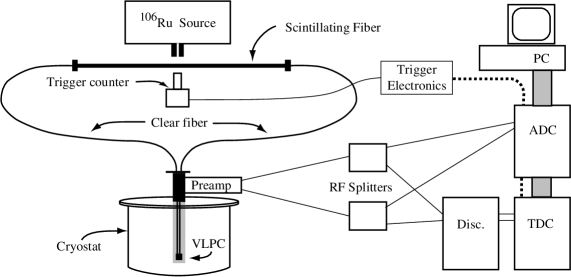
Figure 1: Block diagram of experimental setup for system time resolution studies.

The system timing tests required that scintillating fiber act as the light source to account for light dispersion within the fiber. The fiber was commercial double-clad 3HF scintillating fiber [9] as proposed for the upgraded DØ tracking system. The fiber was instrumented on both ends, with the time difference ($\Delta t$) between receipt of the signal at each end being the quantity of interest. Constraints within the existing DØ detector require that the cryostats containing the VLPC’s be physically separated from the tracking detector, so in some cases a clear fiber of 8 m length was used as a light guide between the scintillating fiber and the cassette containing the VLPC’s. Relevant parameters for the fibers are given in Table 1. Mineral oil was used as the optical coupling between diamond-polished fiber ends within mating connectors.

Table 1: Specifications for scintillating and clear fiber.

		Scintillating Fiber	Clear Fiber
Core	Diameter ($\mu$m)	755	875
	Principle composition	polystyrene	polystyrene
	Dopants	p-terphenyl 1%
		3HF 1500 ppm
	Index of refraction	1.59	1.59
First Cladding	Thickness ($\mu$m)	20	23
	Composition	Acrylic (PMMA)
	Index of Refraction	1.48
Second Cladding	Thickness ($\mu$m)	20	23
	Composition	Fluorinated PMMA
	Index of refraction	1.42

Light was generated within the scintillating fiber by illuminating it with a collimated ¹⁰⁶Ru radioactive source. Ruthenium provides the highest energy beta rays naturally available and was preferred to cosmic ray muons because of the increased event rate. A scintillator paddle instrumented with a photomultiplier tube and located in the fiber’s shadow from the radioactive source served as the system trigger.

In spite of its high gain, the signal from the VLPC must be amplified, especially when used for low light intensities when only a few photoelectrons are produced. In such an application, the amplifier operates in pulse mode, meaning that the time integral of each burst of current, the charge, is converted to a voltage value. This needs to be done with a minimum of additional noise and with sufficient speed to minimize the effect on system time resolution. Measurements of signal pulses directly out of the cassette for high light intensities yielded rise times of 3–5 ns. (Internal rise times within the VLPC may be somewhat faster but the limiting time is that observed outside the cassette. The frequency response of the signal cable within the cassette was measured to drop by 2.5 dB at 100 MHz.) The 3 ns figure yields an equivalent bandwidth of 120 MHz which sets a lower limit on the amplifier’s performance. The final constraint on amplifier performance is the gain necessary to provide sufficient output voltage for the following stages of instrumentation and analysis. Note that it is difficult to obtain acceptable signal-to-noise performance for amplifiers with high gain, high sensitivity, and high bandwidth.

Several amplifiers were tested, but no single device met all constraints. The best results were obtained with a combination of two commercial devices: the Philips NE5211 [10] transimpedance amplifier to convert the current pulse into a voltage pulse followed by the Harris HFA1100 [11] current feedback amplifier to amplify the voltage pulse. The two stage circuit is shown in Fig. 2. The NE5211, as a single device, had better time resolution than the other options but also had relatively low gain which was unacceptable for light intensities below ten detected photons. However, the amplifier’s low input noise combined with its high sensitivity make it desirable as a first stage particle detector preamplifier since the most important noise sources are at the detector front-end. The primary purpose of the second stage was to provide voltage amplification with a minimum impact on the system time resolution. As a current feedback amplifier (or transimpedance amplifier) the HFA1100 is primarily intended for current-to-voltage conversion, but for this test the device was configured as a non-inverting voltage amplifier. The main features of these devices are listed in Table 2.

Figure 2: Schematic of preamplifier circuit used for system timing measurements.

Table 2: Specifications for the commercial amplifiers. The bandwidth of the HFA1100 is given as configured for the amplifier circuit used.

	NE5211	HFA1100
Bandwidth	180 MHz	120 MHz
Input Noise	1.8 $\mathrm{pA}/\sqrt{\mathrm{Hz}}$	4 $\mathrm{nV}/\sqrt{\mathrm{Hz}}$
Input Impedance	200 $\Omega$	10 $\Omega$ (Input –)
		50 K$\Omega$ (Input +)
Input Capacitance	4 pF	2pF
Transimpedance Gain	$R_{T}=28$ k$\Omega$ (differential output)	$R_{T}=500$ k$\Omega$ (open loop)
	$R_{T}=14$ k$\Omega$ (single ended output)

The actual time resolution may be better than that measured because the VLPC signals were split after amplification by the preamplifier. This scheme enabled a simultaneous measurement of both pulse area and time. Resistive splitters with a frequency response flat to within 1 dB for 0–2 GHz were used to minimize phase shifts which would affect time measurements. Splitting the signal resistively provided a 6.3 dB loss in amplitude. The decision to provide the signals to both a TDC and an ADC was motivated by the need to understand the time resolution and the TDC trigger efficiency as a function of the number of photoelectrons present in the event.

A LeCroy 4413 discriminator module [12] with a threshold setting of $\sim$20 mV provided discriminated signals from the VLPC channels to a LeCroy 2228A CAMAC TDC module with a least count of 50 ps for time measurements relative to the system trigger. A LeCroy 2249A CAMAC ADC module integrated the accumulated charge on each tested channel during a gate of 80 ns after a triggered event.

3 Timing Test: Data Analysis and Modelling

Analysis of the system time resolution for a specific configuration was straightforward given the integrated charge and pulse arrival time at each end of the fiber for each event. Rather than relying on the system trigger to provide a reference time, the time difference between signal arrival for each end was measured. The system time resolution was defined as the root mean square (RMS) of the distribution of time differences.

In spite of the collimated source, most triggered events did not produce scintillation photons within the fiber. This was due to the small cross-section presented by the fiber and to ineffectively collimated gamma ray photons and bremsstrahlung x-rays produced by the source. Such events were eliminated by requiring that each end of the fiber yield a signal greater than two standard deviations above pedestal.

Within the resolution of the instruments involved, the pulse area information yielded the number of photoelectrons produced in the VLPC in any given event. The ADC scale was determined from low photon multiplicity events where the pulse area distribution revealed peaks from integer numbers of photoelectrons. The high-bandwidth, high-gain preamplifier used for these tests provided relatively poor pulse area resolution due to noise in the system. This effect contributed to the systematic uncertainty assigned to the measured mean light intensity.

The presence of the ADC information also allowed a determination of the efficiency of the TDC discriminator to trigger on single photoelectron events. Figure 3 is a good example of the integrated charge distribution for one channel for low photon multiplicity events. The solid histogram represents events with a signal ($>$2$\sigma$ above pedestal) present on the opposite end of the fiber. The peaks in the distribution correspond to integer numbers of photoelectrons produced in the VLPC; the first peak is the pedestal which has not been suppressed. The dotted histogram is the distribution after events which had non-physical TDC values were eliminated— either the TDC fired prematurely due to noise in the circuit or did not fire at all. The vertical line is placed at two standard deviations above pedestal; events below this value are removed in the final analysis. With the chosen preamplifier, the TDC discriminator was estimated to have an efficiency of approximately 30% for single photoelectron events relative to the efficiency for events of higher multiplicity.

Figure 3: Integrated charge distribution for low multiplicity events. The dotted histogram is a subset of the solid histogram and shows events for which the TDC found a pulse. The vertical line indicates two standard deviations above the pedestal mean.

A simple Monte Carlo simulation using Mathematica [13] was developed to predict the expected time difference distribution. The model included the light intensity at the VLPC, decay time of the scintillator and wave shifter, dispersion in the fiber, and random noise contributing to premature firing of the TDC’s.

The light intensity for a given set of conditions was derived from the data. The integrated charge for each fiber end was considered separately. Using the measured gain and pedestal mean, the distribution was scaled to yield photoelectron number rather than pulse area. The results from both ends were then combined to give the total number of photoelectrons produced for each event. Within the Monte Carlo, photon production was modeled for the combined total which accounted for correlations between light intensities at each end. It was found that the average light intensity at one end of a fiber was often different from that of the other end. This was assumed to be due to poor optical coupling within one or more of the fiber connectors. Thus within the Monte Carlo, each photon’s longitudinal direction was randomly chosen with a weighting determined by the average light intensities detected at each end. For simplicity, photons were produced according to a Poisson distribution rather than the actual probability function given by the data. The Poisson mean was varied by $\pm 20\%$ from the central value to account for this discrepancy and for the uncertainty in the photoelectron scale. Photon loss in the fiber was not simulated since this is not strongly correlated with the photon’s time of arrival. Figure 4 shows a comparison of the number of photons seen in the data to the Monte Carlo model for the lowest light intensity tests.

Figure 4: The number of events recorded as a function of the number of photoelectrons detected for the longest fiber configuration. The data is depicted by the points; the histogram represents the Monte Carlo. Plot (a) is the combined total from both ends. The lower plots show each end individually.

Within the Monte Carlo simulation, photons were generated with an exponential time distribution in agreement with the exponential decay of the scintillator which has been measured to have a lifetime of $8.2\pm 0.2$ ns. A simple ray tracing algorithm was used to model the time dispersion of photons within the fiber.

The Monte Carlo simulation calculated the time difference between the first detected photons at each end of the fiber after including an overall system time resolution. The measured inefficiency for detecting a single photon was included in the model; the discriminators were assumed to be fully efficient for more than one photoelectron. Studies of the rate of premature firing of the TDC’s in the data prior to the first photon arrival yielded a noise probability which was also included in the simulation.

Photons were assumed to be generated at the axial and longitudinal center of the fiber. Allowing the photons to be generated off-axis yielded an approximate 20% decrease in the average longitudinal distance traveled between bounces assuming a reflection probability of unity for photon paths within the critical angle. The decrease was due to helical photon paths which allow photons to be retained in the fiber with lower longitudinal velocity as shown in the Monte Carlo event depicted in Fig. 5. This effect is largest for long fibers and small photon statistics. However, as shown in Fig. 6, the increased dispersion was not evident in the total time resolution due to the long decay time of the wave shifter which dominated the distribution. Including a reasonable absorption length and coefficient of reflection in the simulation further reduced the effect of the off-axis photons due to the higher probability that these photons are not detected. Thus, off-axis photons were not included since it was felt that the added assumptions yielded only a minor correction which likely exceeded the predictive power of the basic ray-tracing prescription.

Figure 5: Isometric view of fiber showing axial and helical photon paths in a simulated event. The fiber is depicted as an octagonal cylinder with a greatly expanded diameter.

Figure 6: Monte Carlo comparison of the time difference between signal produced at opposite ends of a 20.0 m scintillating fiber for axial photon paths (points) and all photon paths (solid histogram) assuming prompt photon production at the center of the fiber. Also shown is the distribution for events with the decay time of the scintillator and wave-shifter included (dotted histogram). Exactly ten photons were produced in each event.

A comparison of the the time difference spectra from data and Monte Carlo simulation for four different fiber lengths is shown in Fig. 7 with the points representing the data. The Monte Carlo results incorporate a system time resolution of 750 ps which yielded the best overall match to the data. The statistical error on the Monte Carlo prediction is suppressed but is similar in magnitude to that of the data. The measured time resolution agrees with the prediction to within $\sim$25%. Note that the Monte Carlo result is normalized to match the data; only a comparison of the shapes is meaningful. The offset of the mean and the asymmetric shape of the distributions are due to the uneven distribution of light between the two sides. The results of the data analysis for the four different conditions are summarized in Table 3.

Figure 7: Time difference between signals produced by VLPC’s attached to both ends of fiber for a total fiber distance between source and VLPC of (a) 9.8 m, (b) 8.8 m, (c) 1.8 m, (d) 0.8 m. The points with error bars represent the data.

Table 3: Measured time resolutions and configurations.

Fiber length from center (m)		Mean Photoelectrons		Time resolution (ns)
Scintillating	Clear	Left	Right	Data	Monte Carlo
1.5	8.5	3.4	4.4	7.0	8.0
0.5	8.5	6.5	4.0	5.7	7.0
1.5	0.5	12.5	12.5	3.0	2.3
0.5	0.5	13.7	21.4	2.0	1.7

The 20% systematic uncertainty in light intensity was not used for the Monte Carlo results shown in Fig. 7. Figure 8 shows the variation in time resolution for the longest fiber configuration when the light intensity is varied by $\pm 20\%$; the nominal light intensity is given by the points with statistical error bars. While both measurement and simulation show that the time resolution depends strongly on the incident light intensity, this uncertainty does not account for the difference between the prediction and the data. Based on the disagreement observed, which can be attributed to the simplicity of the simulation, predictions of future performance are quoted with a systematic uncertainty of $\pm 50\%$.

Figure 8: Time difference distribution predicted by Monte Carlo for the longest fiber configuration. The points represent the nominal light intensity; the histograms give the result for a variation in light intensity of $\pm 20\%$. The time resolution prediction varies by $\pm 8\%$.

4 Timing Test: Discussion

The longitudinal position resolution for a charged particle impacting a fiber detector is a linear function of the system time resolution,

$$\sigma_{p}=K(I)\frac{c}{2n}\sigma_{t}$$

where $c$ is the speed of light and $n$ is the refractive index of the fiber. The factor $K$ is a function of the light intensity, and in this application represents the deviation of the average longitudinal speed of the first detected photon from the speed of light in the fiber, assuming an even distribution of light. The Monte Carlo model described above indicates that for the lowest possible light intensity with the standard fiber, one detected photon on each end, $K\approx 0.96$. The value of $K$ approaches unity with increasing light intensity with $K\approx 0.99$ for ten total photoelectrons. The following discussion assumes $K=1$.

Tests with cosmic ray muons indicate that a minimum ionizing particle typically produces $\sim$10 total photoelectrons for the longest fiber configuration tested here. The results given above then indicate a position resolution of $\sim$60 cm for a minimum ionizing particle. Thus time measurements are not a reasonable option for longitudinal position determination in the type of detector constructed for these tests.

Comparison of the simulation with the data suggests that the dominant effects determining the time resolution of the system are the light intensity and the decay time of the scintillator. Time dispersion of photons within the fiber is of secondary importance. Thus, dramatic improvements would arise from a faster wave-shifter or more light production. Furthermore, a new version of the VLPC, HISTE-V, has a factor of $\sim$2.5 higher gain which should provide 100% efficiency for time measurements with a single photoelectron; this should effect a modest improvement in time resolution for low multiplicity events.

The preceding observations motivated a final set of simulations yielding predictions of the time resolution as a function of total number of photoelectrons produced for two detector configurations: the first using the 3HF fiber, the second using commercially available green scintillating fiber with a decay time of 2.7 ns. Unfortunately, the fast scintillating fibers that are available have attenuation lengths that are small compared to the 3HF fiber. The results are shown in Fig. 9. These results follow from the ideal case where the electronics time resolution is negligible and the TDC’s are assumed to be 100% efficient for detecting a single photoelectron. The photons were assumed to be produced in the longitudinal center of a fiber of total length 20 m.

These final results provide information necessary to understand the effectiveness of using time difference measurements to determine the longitudinal position of a particle or shower in a scintillator detector. As an example, the central fiber tracker proposed for the DØ upgrade will be constructed of scintillating fiber identical to the standard fiber described in Table 1. For a single fiber, the expected ten photoelectrons produced by a minimum ionizing particle yield an RMS longitudinal position resolution of $\sim$50 cm. DØ’s proposed tracking detector would eliminate gaps by densely packing two layers of fibers for each superlayer. Instrumenting fiber doublets would then increase the mean number of photoelectrons to 20 and should improve the position resolution to $\sim$27 cm for each superlayer. This resolution could be useful to eliminate combinatoric background in a tracking-based trigger. As another example, the central preshower detector proposed for the DØ upgrade is expected to have a minimum trigger threshold of $\sim$80 photoelectrons for electron candidates [14]. Using wavelength shifting fiber with the same fluorescence decay time as that used for the tracker would yield an RMS longitudinal position resolution of $\sim$12 cm. This resolution is acceptable for certain trigger requirements and, like all of the scenarios discussed here, could be dramatically improved by using fiber with a faster decay time.

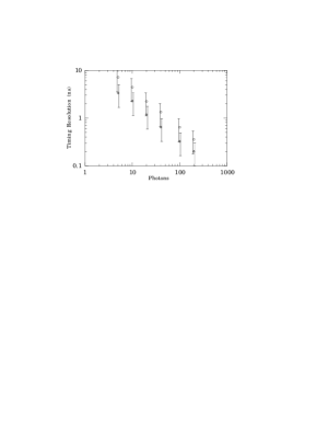
Figure 9: Monte Carlo prediction of expected time resolution for future systems. The circles are for the standard fiber described above. The diamonds are for scintillating fiber with a faster fluorescence decay time of 2.7 ns. The error bars are offset for clarity and denote the assigned 50% systematic error.

5 Gain Linearity Test: Experimental Setup

The linearity tests shared the VLPC cassette and cryogenic system with the timing tests; other details of the system differed. A block diagram of the experimental setup is shown in Fig. 10.

Figure 10: Block diagram of experimental setup for VLPC gain linearity studies.

Because timing was not an issue for this study, bulk scintillator with the same composition as the fiber core was used as the light source. A schematic of the light source is shown in Fig. 11. The scintillator was illuminated with an ultraviolet (UV) nitrogen laser producing pulsed light ($\lambda$ = 337.1 nm) with a width of 3 ns at a frequency of 10 Hz. The UV light activated the wavelength shifting component of the scintillator which subsequently produced visible light. This configuration provided a constant intensity light source with the appropriate wavelength spectrum. The low pulse frequency ensured adequate recovery time for the VLPC. Absorptive neutral density filters (NDF’s) attenuated the light by known factors and served as the reference by which linearity was judged. A liquid light guide transported the light from the source to the VLPC cassette.

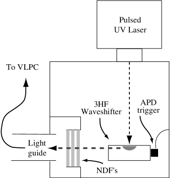
Figure 11: Block diagram of the light source used for VLPC gain linearity studies.

Three preamplifier configurations were used to ensure that the limited dynamic range of any single amplifier did not affect the measurement. The highest gain preamplifier was similar to that used for the timing tests but lacked the second stage of amplification; this improved its dynamic range. The mid-gain preamplifier was of the same design but attenuated the signal from the VLPC at the input. The lowest gain “preamp” was a circuit allowing the VLPC to be directly read by the input stage of the digital signal analyzer. Thus, the signal was not amplified at all, and any saturation seen at this point was due to the VLPC rather than any intervening electronics. Figure 12 shows a schematic of the low gain circuit.

Figure 12: Schematic of the circuit used to connect the digital signal analyzer directly to the VLPC for the gain linearity studies.

A commercial digital signal analyzer (DSA), Tektronix model DSA 602A [15], was used to integrate the charge from the output stage of the preamplifier. The signal was averaged over the 512 events prior to the measurement with the systematic uncertainty being determined by varying the gate width from 40 ns to 80 ns. The measurement error of the DSA was small compared to the systematic uncertainty assigned to the measurement.

The photoelectron scale was set in the same manner as described above for the timing measurements using a CAMAC ADC to record the integrated charge distribution for the lowest intensity configuration. The mean number of photoelectrons from this distribution then served as the reference for all configurations since the filters attenuated the signal by a known amount. A 10% uncertainty was assigned to the optical density of the filters in accordance with the manufacturer’s specifications. The measurement of the mean number of photoelectrons for the reference configuration was assigned a systematic uncertainty of 15% which is fully correlated for all points.

6 Linearity Test: Results and Discussion

Two channels contributed to the linearity measurement. Figure 13 shows the response of the VLPC as a function of the number of photoelectrons produced for one channel. Figure 14 shows the percent deviation from linearity for the same channel. The uncorrelated uncertainties are given by the error bars; there is an additional 15% uncertainty in the photoelectron scale. This VLPC is linear to within 10% out to $\sim$600 photoelectrons. A similar result was obtained from the other tested channel.

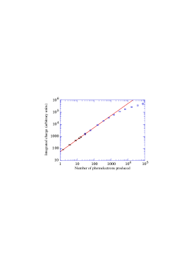
Figure 13: VLPC response vs. input photoelectrons.

Figure 14: Percent deviation from linearity for VLPC vs. input photoelectrons. Data from all three tested preamp configurations are shown.

The VLPC provides high gain due to fast avalanche multiplication of charge within the device. As described in the literature [16, 17], the avalanche produces a space charge in a small area inhibiting subsequent avalanches within the recovery time of the device which could be as long as 1 ms. A Monte Carlo model was developed to characterize the surface size of two idealized regions: a small region for which subsequent avalanches were fully inhibited yielding a dead area, and a larger region for which the average gain for subsequent avalanches was reduced by 10%. The model assumed that the affected regions were circular, and that the recovery time of the device was long compared to the time distribution of photons in a given event. To characterize the size of the smaller region, it was assumed that the avalance due to a single photoelectron left the circular area completely dead for subsequent photons. In such a model, complete coverage of the active area of the VLPC would result in saturation. Assuming that full saturation begins for $\sim$1$\times 10^{5}$ photoelectrons as suggested by Fig. 13, the simulation reveals the radius of the dead region to be 1 $\mu$m. This is consistent with theoretical calculations [18]. The small size of the dead region also suggests an explanation for the deviation from linearity that is observed to begin at $\sim$600 photoelectrons. Since the gain region is only 5 $\mu$m thick, the space charge is concentrated in a region that is only 1–2 $\mu$m on a side. This clump of positive charge will then distort the local field causing some loss of amplification for nearby photoelectrons that are outside the dead region. For an average gain reduction of 10%, the same Monte Carlo model was used to estimate the diameter of the affected circular region at 23 $\mu$m. This result must be interpreted as the average cut-off diameter since the model assumes a rigid cut-off whereas the field distortion will likely cause a continuous reduction in gain. The results given by this model allow a prediction of VLPC linearity for systems with different coverage of VLPC pixels than the apparatus described here.

These results indicate that the VLPC is an ideal device for calorimetric applications. It can provide high sensitivity and can accept large incident light intensities.

7 Conclusion

The time resolution was measured for a scintillating fiber detector instrumented on both ends with HISTE-IV VLPC’s operated at 6.5 K and with a bias voltage of 6.5 V. The measurements were shown to agree with predictions from a simple Monte Carlo simulation incorporating only the decay time of the scintillator, the mean light intensity, and the dispersion in the fiber as modeled with a simple ray-tracing algorithm. The light intensity coupled with the decay time of the scintillator clearly dominates the resolution. The results of the study suggest that time difference measurements are not attractive for longitudinal position measurements in single fibers unless the fiber has a short fluorescence decay time ($\lesssim$2 ns). Higher light intensities (which are expected in electromagnetic showers) provide a more acceptable position resolution.

Measurements also addressed the linearity of HISTE-IV VLPC’s over a wide range of incident light intensities. With a bias voltage of 6.5 V at 6.5 K, the VLPC was shown to have a linear response up to $\sim$600 photoelectrons, and the VLPC output continued to increase monotonically up to incident light intensities producing at least $7\times 10^{4}$ photoelectrons.

8 Acknowledgements

Technical assistance for this project was provided by the DØ department of the Fermilab Research Division. The authors acknowledge the support provided by the U.S. Department of Energy, the University of Maryland, and CNPq in Brazil.

References

- [1] R.C. Ruchti, Ann. Rev. Nucl. Part. Sci. 46 (1996) 281.
- [2] M.D. Petroff, M.G. Stapelbroek, and W.A. Kleinhans, Appl. Phys. Lett. (1987) 406.
- [3] Rockwell International Science Center, Anaheim, California.
- [4] The measurements reported are valid only for the Rockwell HISTE-IV model VLPC operating under the conditions specified.
- [5] D. Adams, et. al., Nuclear Physics B (Proc. Suppl.), 44 (1995) 340.
- [6] D. Adams, et. al., Nuclear Physics B (Proc. Suppl.), 44 (1995) 332.
- [7] N.A. Amos, A.D. Bross and M.C. Lundin, Nucl. Inst. and Methods A 297 (1990) 396.
- [8] A. Bross, private communication, Sep. 1995.
- [9] R. Ruchti, in: SCIFI 93 Workshop on Scintillating Fiber Detectors, eds. A.D. Bross, R.C. Ruchti, and M.R. Wayne, (World Scientific, River Edge, NJ, 1995) pp. 126-139.
- [10] Philips Semiconductor Sunnyvale, CA.
- [11] Harris Semiconductor, Melbourne, CA.
- [12] LeCroy Corporation, Chestnut Ridge, NY.
- [13] Mathematica is a product of Wolfram Research, Urbana, IL.
- [14] D. Lincoln, private communication, Sep. 1995.
- [15] Tektronix Inc., Beaverton, OR.
- [16] G.B. Turner, M.G. Stapelbroek, M.D. Petroff, E.W. Atkins, and H.H. Hogue, in: SCIFI 93 Workshop on Scintillating Fiber Detectors, eds. A.D. Bross, R.C. Ruchti, and M.R. Wayne, (World Scientific, River Edge, NJ, 1995) pp. 613-620.
- [17] M.G. Stapelbroek and M.D. Petroff, in: SCIFI 93 Workshop on Scintillating Fiber Detectors, eds. A.D. Bross, R.C. Ruchti, and M.R. Wayne, (World Scientific, River Edge, NJ, 1995) pp. 621-629.
- [18] M. G. Stapelbroek, private communication, Oct. 1995.