Fermilab-Conf-96/354 November 1996

Precision Electroweak Measurements

Marcel Demarteau Fermilab

Batavia, IL 60510, USA

Recent electroweak precision measurements from $e^{+}e^{-}$ and $\overline{p}p$ colliders are presented. Some emphasis is placed on the recent developments in the heavy flavor sector. The measurements are compared to predictions from the Standard Model of electroweak interactions. All results are found to be consistent with the Standard Model. The indirect constraint on the top quark mass from all measurements is in excellent agreement with the direct $m_{\mathrm{t}}$ measurements. Using the world’s electroweak data in conjunction with the current measurement of the top quark mass, the constraints on the Higgs mass are discussed.

Recent electroweak precision measurements from $e^{+}e^{-}$ and $\overline{p}p$ colliders are presented. Some emphasis is placed on the recent developments in the heavy flavor sector. The measurements are compared to predictions from the Standard Model of electroweak interactions. All results are found to be consistent with the Standard Model. The indirect constraint on the top quark mass from all measurements is in excellent agreement with the direct $m_{\mathrm{t}}$ measurements. Using the world’s electroweak data in conjunction with the current measurement of the top quark mass, the constraints on the Higgs mass are discussed.

1 Introduction

Radiative corrections in the standard model of electroweak interactions (Standard Model) have taken a very prominent position in today’s description of experimental results. Perhaps the most compelling reason for this state of affairs is that the experimental results have reached a level of precision which require a comparison with theory beyond the Born calculations, which the Standard Model is able to provide. If loop calculations are needed for the calculation of physics observables, the measurements show sensitivity to the masses and couplings of the particles propagating in the loops. The experimental measurements can thus provide information about the particles contributing to the radiative corrections well below the threshold for directly producing them.

In this summary the most recent electroweak results from $e^{+}e^{-}$ and $\overline{p}p$ colliders will be described. The emphasis will be on electroweak results from data taken on the $Z$ resonance. Within the Standard Model, the description of all processes involving neutral currents is given in terms of the chiral couplings of the fermion $f$ to the $Z$ boson, $g_{L}^{f}$ and $g_{R}^{f}$, or more commonly in terms of the vector and axial-vector couplings, $g_{V}^{f}$ and $g_{V}^{f}$:

$$g_{V}^{f}= (g_{L}^{f}\,+\,g_{R}^{f})= I^{f}_{3}\,-\,2\,Q_{f}\,\sin^{2}\vartheta_{W}$$

$$g_{A}^{f}= (g_{L}^{f}\,-\,g_{R}^{f})= I^{f}_{3}\ .$$

Here $\vartheta_{W}$ is the weak mixing angle, $I^{f}_{3}$ the weak isospin component of fermion $f$ and $Q_{f}$ its charge.

Because the left-handed and right-handed coupling of fermions to the $Z$ boson are not the same, the angular distribution of the outgoing fermion with respect to the incoming fermion in the center of mass frame for the process $\mbox{$e^{+}e^{-}$}\rightarrow\mbox{$f\overline{f}$ }$ has a term linear in $\cos(\vartheta)$ [1]. The distribution is thus asymmetric and will exhibit a forward-backward asymmetry, defined as

$$A_{\mathrm{FB}}\,=\,{\sigma_{F}\,-\,\sigma_{B}\over\sigma_{F}\,+\,\sigma_{B}}\ ,$$

where $\sigma_{F}$ is the cross section for fermion production in the forward hemisphere ($0^{\circ}<\vartheta<90^{\circ}$) and $\sigma_{B}$ the cross section for the backward hemisphere ($90^{\circ}<\vartheta<180^{\circ}$).

Around the $Z$ pole, the photon exchange and $\gamma Z$ interference are only small corrections to the resonance cross section. Retaining only the resonance cross section, the forward-backward asymmetry on the pole is, at lowest order, given by

$$A^{0,\,\ell}_{\rm{FB}}\,=\,{3\over 4}\,{\cal A}_{e}\,{\cal A}_{\ell}\ ,$$

where the asymmetry of couplings, $\cal A_{\rm f}$, are given by

$$\mbox{$\cal A_{\rm f}$}\,\equiv\,{{g_{L}^{f}}^{2}\,-\,{g_{R}^{f}}^{2}\over{g_{L}^{f}}^{2}\,+\,{g_{R}^{f}}^{2}}\,=\,{2\,g_{V}^{f}\,g_{A}^{f}\over{g_{V}^{f}}^{2}\,+\,{g_{A}^{f}}^{2}}\ .$$

These expressions will be modified when including higher order corrections. Weak vertex corrections and self-energy diagrams will introduce fermion dependent form factors which can be absorbed in the definition of the coupling constants [2]. By introducing effective coupling constants the Born structure of the processes can to a good approximation be retained. Since all asymmetry measurements determine essentially the ratio of couplings ${g_{V}^{f}}/{g_{A}^{f}}$ it is convenient to define an effective electroweak mixing angle

$$\sin^{2}\!\theta_{\rm{eff}}^{\rm{lept}}\,\equiv\,{1\over 4}\,\left(1-{{g_{V}^{f}}^{2}\over{g_{A}^{f}}^{2}}\right)\ \ ,$$

which is well matched with the quantities measured experimentally. The effective electroweak mixing angle is, coincidentally, very close to the definition in the ${\overline{\rm MS}}$ scheme [3].

The results presented are based on event samples of about $4\cdot 10^{5}$ leptonic and $3.5\cdot 10^{6}$ hadronic $Z$ decays per LEP experiment, complemented with $1.6\cdot 10^{5}$ $Z$ decays recorded at SLC with a polarized electron beam. The $\overline{p}p$ experiments CDF and DØ each have approximately 60,000 leptonic $W$ and 6000 leptonic $Z$ decays collected during the 1992-1993 run (Run 1a) and the 1994-1995 run (Run 1b) combined. A fivefold increase in luminosity was obtained in the latter run. All results presented are preliminary.

In the next section results from line shape measurements will be described. The results on the effective coupling constants from the line shape measurements and the forward-backward asymmetries in the leptonic sector will be summarized in section 2.3. The section following describes the main developments in the hadronic sector with the emphasis on $R_{\mathrm{b}}$ and $R_{\mathrm{c}}$. Given the full set of measurements, an overall fit is performed within the framework of the Standard Model and the consistency of the results verified. We will conclude with some recent developments.

2 Line shapes and Asymmetries

2.1 Line shape Measurements

In $\overline{p}p$ and $e^{+}e^{-}$ collisions final state lepton pairs are produced through photon and $Z$ exchange. The cross section at lowest order is given by

$$\sigma_{ff} \propto {12\pi\over M_{Z}^{2}}\,{\Gamma_{ee}\Gamma_{ff}\over\Gamma_{Z}^{2}}\,{s\,\Gamma_{Z}^{2}\over(s-M_{Z}^{2})^{2}\,+\,s^{2}\Gamma_{Z}^{2}/M_{Z}^{2}}$$

$$+\,``\gamma Z"\,+\,``\gamma"$$

consisting of the $Z$ resonance cross section, the QED annihilation term (“$\gamma$”) and the $\gamma Z$ interference term (“$\gamma Z$”). At proton colliders the resonance cross section for $W$ and $Z$ production is used to indirectly determine the width of the $W$ boson through the ratio of the $W$ and $Z$ production cross sections. At $e^{+}e^{-}$ colliders the measurement of the resonance line shape is used to extract $m_{\mathrm{Z}}$ and $\Gamma_{\mathrm{Z}}$. Figure 1 shows the hadronic resonant cross section as measured by the L3 experiment. From the hadronic decays of the $Z$ boson the hadronic pole cross section, $\sigma_{\mathrm{h}}^{0}\equiv{12\pi\over M_{Z}^{2}}\,{\Gamma_{ee}\Gamma_{\rm had}\over\Gamma_{Z}^{2}}$ is determined. From the leptonic decays the ratio of the partial hadronic and leptonic widths, $R_{\ell}\equiv{\Gamma_{\mathrm{had}}\over\Gamma_{\ell\ell}}$, is derived. This particular choice of variables, $m_{\mathrm{Z}},\Gamma_{\mathrm{Z}},\sigma_{\mathrm{h}}^{0}$ and $R_{\ell}$, is motivated by the desire to minimize the correlation among the variables and to minimize any model dependence. One of the main challenges of these measurements is to control the systematic uncertainties and keep them at the same level as the statistical uncertainties. Since the measurements of these quantities entail both an absolute cross section measurement and an absolute mass determination, the luminosity and energy calibration are crucial.

The LEP experiments all measure the luminosity with small angle silicon based calorimeters with good spatial resolution counting Bhabha events. At small scattering angles $\vartheta$, the cross section for Bhabha scattering shows a $\vartheta^{-3}$ dependence. For the luminosity measurement a very precise knowledge of the edges of the acceptance is required. An accuracy of 10 $\mu$m is currently achieved, resulting in an uncertainty of $\delta({\cal L})\approx(0.07-0.15)$%, surpassing the theoretical uncertainty [4]. Recent advances in the calculation of the Bhabha cross section [5] have significantly reduced the theoretical uncertainty on the luminosity to the level of 0.11%, with a further reduction of a factor of two anticipated in the near future.

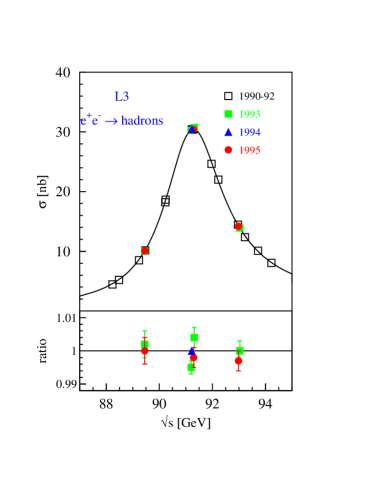
Figure 1: Hadronic resonant cross section as function of $\sqrt{s}$ as measured by L3 (top) and the comparison with the theoretical prediction (bottom).

The calibration of the LEP beam energy is a remarkable feat. The beam energy is measured most accurately using the technique of resonant depolarization which has an ultimate accuracy of about 200 keV. This calibration, however, cannot be performed very often since it takes a long time for the transverse beam polarization to build up in the accelerator. Moreover, it cannot be done during a physics run and has been performed with separated beams only. The energy of the beam is generally tracked using NMR probes. Over the course of the years it was discovered that the circumference of the LEP tunnel, and thus the beam energy, was sensitive to the water level of Lake Geneva and the phases of the moon. The sun and moon tides changed the LEP orbit by up to 1 mm [6]. In 1995 NMR probes were installed inside two of the LEP magnets in the tunnel and a new puzzle arose. It was observed that there were large fluctuations in the beam energy which magically disappeared at midnight only to show up again shortly after 4am each day. This effect was eventually traced to an induction voltage on the LEP beam pipe caused by vagabond currents on the TGV train track rails (see Fig. 2) [6]. All these effects have been taken into account for the results presented here and propagated back into the previous years with a resulting uncertainty on the $Z$ mass and width of $\Delta M_{Z}$ = 1.5 MeV/c² and $\Delta\Gamma_{Z}$ = 1.7 MeV.

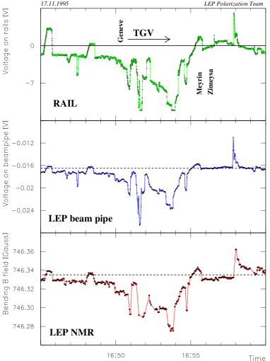
Figure 2: From top to bottom: voltage on the rails, voltage on the beampipe and dipole field strength over a period of 15 minutes while the TGV travels closest to the LEP tunnel.

	ALEPH		DELPHI		L3		OPAL		Average Value
$m_{\mathrm{Z}}({\mathrm{Ge\kern-1.00006ptV}})$	$91.1873$$\pm$	$0.0030$	$91.1859$$\pm$	$0.0028$	$91.1883$$\pm$	$0.0029$	$91.1824$$\pm$	$0.0039$	$91.1863$$\pm$	$0.0020$
$\Gamma_{\mathrm{Z}}({\mathrm{Ge\kern-1.00006ptV}})$	$2.4950$$\pm$	$0.0047$	$2.4896$$\pm$	$0.0042$	$2.4996$$\pm$	$0.0043$	$2.4956$$\pm$	$0.0053$	$2.4946$$\pm$	$0.0027$
$\sigma_{\mathrm{h}}^{0}(\rm{nb})$	$41.576$$\pm$	$0.083$	$41.566$$\pm$	$0.079$	$41.411$$\pm$	$0.074$	$41.53$$\pm$	$0.09$	$41.508$$\pm$	$0.056$
$R_{e}$	$20.64$$\pm$	$0.09$	$20.93$$\pm$	$0.14$	$20.78$$\pm$	$0.11$	$20.82$$\pm$	$0.14$	$20.754$$\pm$	$0.057$
$R_{\mu}$	$20.88$$\pm$	$0.07$	$20.70$$\pm$	$0.09$	$20.84$$\pm$	$0.10$	$20.79$$\pm$	$0.07$	$20.796$$\pm$	$0.040$
$R_{\tau}$	$20.78$$\pm$	$0.08$	$20.78$$\pm$	$0.15$	$20.75$$\pm$	$0.14$	$20.99$$\pm$	$0.12$	$20.814$$\pm$	$0.055$
$A^{0,\,{\rm e}}_{\rm{FB}}$	$0.0187$$\pm$	$0.0039$	$0.0179$$\pm$	$0.0051$	$0.0148$$\pm$	$0.0063$	$0.0104$$\pm$	$0.0052$	$0.0160$$\pm$	$0.0024$
$A^{0,\,\mu}_{\rm{FB}}$	$0.0179$$\pm$	$0.0025$	$0.0153$$\pm$	$0.0026$	$0.0176$$\pm$	$0.0035$	$0.0146$$\pm$	$0.0025$	$0.0162$$\pm$	$0.0013$
$A^{0,\,\tau}_{\rm{FB}}$	$0.0196$$\pm$	$0.0028$	$0.0223$$\pm$	$0.0039$	$0.0233$$\pm$	$0.0049$	$0.0178$$\pm$	$0.0034$	$0.0201$$\pm$	$0.0018$

Table 1: Line shape and asymmetry parameters from 9-parameter fits to the data of the four LEP experiments. The last column gives the LEP averages.

The results of the line shape measurements of the four LEP experiments are given in the first 6 rows of Table 1. The last column lists the LEP averages. The accuracy of the measurements is impressive. It should be noted that the effects of radiative corrections are applied within the framework of the Standard Model. For example, initial state radiation, which shifts the peak cross section by $\sim$ 89 MeV and reduces it by $\sim$ 26%, are taken into account through QED radiator functions.

In $\overline{p}p$ collisions the lineshape of the $Z$ resonance is also probed. Because of the large range of available partonic center of mass energies the Drell-Yan process ($\mathrm{q}\overline{\mathrm{q}}\rightarrow(\gamma,Z\rightarrow)\ \ell^{+}\ell^{-})$ can be studied over a large di-lepton invariant mass region. The invariant mass region well above the $Z$ pole is the region where the $\gamma Z$ interference effects are strongest. A possible substructure of the partons would manifest itself most prominently in a modification of the interference pattern. Substructure of partons is most commonly parametrized in terms of a contact interaction characterized by a phase, $\eta$, leading to constructive ($\eta=-1$) or destructive interference ($\eta=+1$) with the Standard Model Lagrangian, and a compositeness scale, $\Lambda_{\eta}$ [7]. By fitting the di-lepton invariant mass spectrum to various assumptions for the compositeness scale and the phase of the interference, lower limits on the compositeness scale can be set.

The CDF experiment has measured the double differential Drell-Yan cross section $d^{2}\sigma/dM\,dy$ for electron and muon pairs in the mass range $11<M_{\ell\ell}<150$ GeV/c² for the Run 1a data [8], and $40<M_{\ell\ell}<550$ GeV/c² for the Run 1b data. Figure 3 shows the measured cross section for electrons and muons combined together with the theoretical predictions. The theory curves correspond to a calculation of the Drell-Yan cross section with in addition a contact interaction of left-handed quarks and leptons with positive interference for different values of the compositeness scale. The curve for $\Lambda_{-}=1000$ TeV indicates the Standard Model prediction. A maximum likelihood fit of the combined electron and muon data to the predictions yields lower limits in the scale factors of $\Lambda_{+}$ $\geq$ 2.9 TeV and $\Lambda_{-}$ $\geq$ 3.8 TeV. This implies that up to a distance of $<10^{-17}$ cm the interacting particles reveal no substructure.

At $e^{+}e^{-}$ colliders particle substructure is also probed using the angular distribution of the final state leptons in the energy range $\sqrt{s}=130-140$ GeV with similar limits [9].

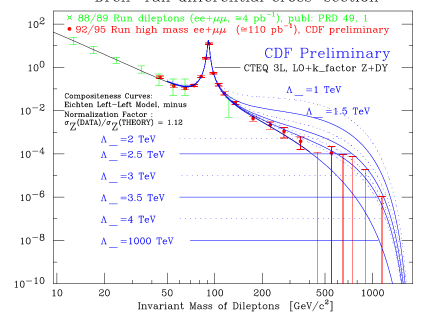
Figure 3: Double differential cross section $d^{2}\sigma/dM\,dy$ for CDF electron and muon data combined. The open symbols are from the 88/89 data. The solid symbols correspond to the full Run I data. The curves are the theoretical predictions for different $\Lambda_{-}$ values.

Another very important line shape which yields a mass measurement [10] is the distribution in transverse mass of $W\rightarrow\ell\nu$ decays. Until very recently the mass of the $W$ boson could only be measured directly in $\overline{p}p$ collisions. In a $W$ event originating from a $\overline{p}p$ interaction in essence only two quantities are measured: the lepton momentum and the transverse momentum of the recoil system. The latter consists of the “hard” $W$-recoil and the underlying event contribution, which for $W$-events are inseparable. The transverse momentum of the neutrino is inferred from these two observables. Since the longitudinal momentum of the neutrino cannot be determined unambiguously, the $W$-boson mass is determined using the transverse mass:

$$m_{T}\,=\,\sqrt{2\,p_{T}^{e}\,p_{T}^{\nu}\,(1-\cos\varphi^{e\nu})}\ ,$$

where $\varphi^{e\nu}$ is the angle between the electron and neutrino in the transverse plane. This distribution exhibits a Jacobian edge, characteristic of two-body decays, which contains most of the mass information.

As in the measurement of the $Z$ mass, knowledge of the absolute energy scale is crucial. At LEP the experiments calibrate to the energy of the beams, which is known with high precision. The Tevatron experiments calibrate to known resonances. In the CDF $W$-mass analysis [11], the momentum scale of the central magnetic tracker is set by scaling the measured $J/\psi$-mass, based on an event sample of approximately 60,000 events, to the world average value using $J/\psi\rightarrow\mu^{+}\mu^{-}$ decays. This procedure establishes the momentum scale at the $J/\psi$-mass, where the average muon $p_{T}$ is about 3 GeV/c, and needs to be extrapolated to the momentum range appropriate for leptons from $W$-decays. The error due to possible nonlinearities in the momentum scale is addressed by studying the measured $J/\psi$-mass as function of $\langle 1/p_{T}^{2}\rangle$, extrapolated to zero curvature. Having established the momentum scale, the calorimeter energy scale is determined from a line shape comparison of the observed $E/p$ distribution with a detailed Monte Carlo prediction.

In the DØ $W$-mass analysis [12] the electromagnetic energy scale is set by calibrating to the $Z\rightarrow ee$ resonance. The quantity measured is essentially the ratio of the measured $W$ and $Z$ mass and the world average $Z$ mass is used to determine the $W$ boson mass. By measuring a ratio a number of systematic effects common to both measurements cancel. Most notably, the ratio is to first order insensitive to the absolute energy scale. The linearity of the calorimeter is addressed by combining the measurement of the $Z$ mass with measurements of the decays $J/\psi\rightarrow e^{+}e^{-}$ and $\pi^{0}\rightarrow\gamma\gamma\rightarrow e^{+}e^{-}e^{+}e^{-}$.

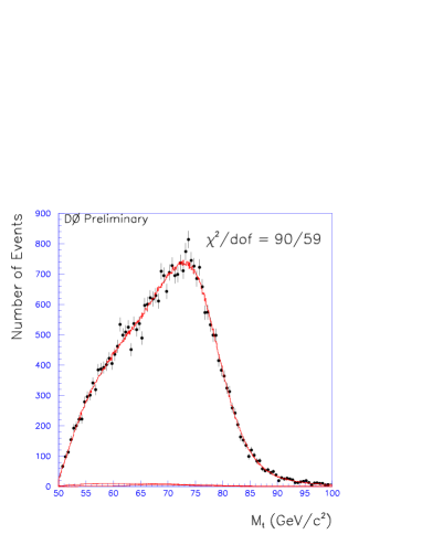
Figure 4: DØ transverse mass distribution for $W\rightarrow e\nu$ events for the Run 1b data. The points are the data and the line is the best fit to the data. The dashed line indicates the background contribution.

Since there is no analytic description of the transverse mass distribution, the $W$-mass is determined by fitting Monte Carlo generated templates in transverse mass for different masses of the $W$-boson to the data distribution. Figure 4 shows the transverse mass distributions for the data together with the best fit of the Monte Carlo for the Run Ib electron data for DØ. The $W$ mass is obtained, using central leptons only, from a fit in transverse mass over a range $60<m_{T}<90$ GeV/c² for DØ and $65<m_{T}<100$ GeV/c² for CDF. The $W$-mass values obtained are $M_{W}^{\mu}=80.310\pm 0.205(stat)\pm 0.130(sys)$ GeV/c², based on 3268 $W\rightarrow\mu\nu$ events in the mass fitting window, and $M_{W}^{e}=80.490\pm 0.145(stat)\pm 0.175(sys)$ GeV/c², based on 5718 events, for CDF using the MRSD^′- parton distribution function (pdf). DØ finds $M_{W}^{e}=80.350\pm 0.140\ {\rm(stat.)}\pm 0.165\ {\rm(syst.)}\pm 0.160\ {\rm(scale)}$ GeV/c², based on 5982 events in the mass fitting window using the Ia data, and $M_{W}^{e}=80.380\pm 0.070\ {\rm(stat.)}\pm 0.130\ {\rm(syst.)}\pm 0.080\ {\rm(scale)}$ GeV/c², based on 27040 events for the Ib data [13]. Both DØ measurements are quoted using the MRSA pdf. Table 2 lists the systematic and common errors on the measurements.

	CDF			DØ
	e	$\mu$	common	Ia	Ib	common
Statistical	145	205	—	140	70	—
Energy scale	120	50	50	160	80	25
Angle scale	—	—	—	50	40	40
$E$ or $p$ resolution	80	60	—	70	25	10
$p_{T}^{W}$ and recoil model	80	75	65	110	95
pdf’s	50	50	50	65	65	65
QCD/QED corr’s	30	30	30	20	20	20
$W$-width	20	20	20	20	10	10
Backgrounds	10	25	—	35	15	—
Efficiencies	0	25	—	30	25	—
Fitting procedure	10	10	—	5	5	—
Total	230	240	100	270	170	80
Combined	180			150

Table 2: Errors on $M_{W}$ in MeV/c².

From the table it can been seen that the error due to the $p_{T}^{W}$ and recoil model and the proton structure are the dominant ones. The fact that there are spectator interactions, multiple interactions and pile-up, with their associated fluctuations and uncertainties, is reflected in the recoil modeling. It is controlled through the study of $Z$ events and is expected to scale with the $Z$ statistics. The uncertainty due to the parton distribution inside the proton is constrained in part by the measurement of the $W$ charge asymmetry [14]. The CDF experiment uses this measurement as the sole constraint on the uncertainty due to the $p_{T}^{W}$ and parton distribution functions. The DØ experiment addresses the correlation between the parton distributions and the spectrum in $p_{T}^{W}$ by varying both the $p_{T}^{W}$ input spectrum and the parton distribution functions simultaneously. This uncertainty is the dominant theoretical uncertainty which is not expected to scale with event statistics.

Combining [15] these measurements with previous $W$ mass measurements [16], assuming the only correlated uncertainty between the measurements from different experiments is due to the parton distribution functions, gives a world average of $M_{W}=80.356\pm 0.125$ GeV/c². Since the mass of the $W$-boson is one of the fundamental parameters of the Standard Model, a precision measurement of the $W$-boson mass can be used to look for inconsistencies between the different measurements and the theoretical predictions, possibly indicating processes beyond the Standard Model. The direct $W$ mass measurements will be confronted with the prediction from the world’s data in section 4.

2.2 Forward-Backward Asymmetry

The forward-backward asymmetries for leptonic $Z$ decays essentially measure the single parameter $\sin^{2}\!\theta_{\rm{eff}}^{\rm{lept}}$. The LEP experiments have measured $A_{\mathrm{FB}}$ both on-pole and off-pole. The off-pole measurements are shifted to the pole center of mass energy using the Standard Model predicted dependence. This is justified since the slope of the asymmetry around $m_{\mathrm{Z}}$ depends only on the axial coupling and the charge of the initial and final state fermions and is thus independent of the value of the asymmetry itself. Figure 5 shows the comparison of the $A^{0,\,\ell}_{\rm{FB}}$ measurements, assuming lepton universality, with the Standard Model prediction. The Standard Model prediction with its uncertainty is given as function of $m_{\mathrm{t}}$. In this figure, and in Fig. 13, three sources of uncertainty on the prediction are indicated by bands. Moving outward from the central value they correspond to the uncertainty on $m_{\mathrm{Z}}$, $\alpha_{s}(m_{\mathrm{Z}}^{2})$ and $m_{\mathrm{H}}$, respectively. The average value is $A^{0,\,\ell}_{\rm{FB}}=0.0174\pm 0.0010$ to be compared to the Standard Model prediction of $A^{0,\,\ell}_{\rm{FB}}=0.0159$ .

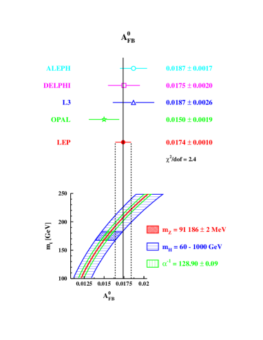
Figure 5: $A^{0,\,\ell}_{\rm{FB}}$ measurements of the LEP experiments and their average compared to the Standard Model prediction

2.3 Results from Lineshape and Forward-Backward Asymmetry

Once the $Z$ lineshape parameters, the forward-backward asymmetries and the center of mass energies are determined, the results are unfolded for initial state radiation and interference effects. That is, the $\gamma$-exchange contributions and the $\gamma Z$ interference terms are fixed to their Standard Model values. Each LEP experiment then performs a fit of the measured quantities in terms of 9 variables, $m_{\mathrm{Z}}$, $\Gamma_{\mathrm{Z}}$, $\sigma_{\mathrm{h}}^{0}$, $R_{\ell}$ and $A^{0,\,\ell}_{\rm{FB}}$. This particular choice of variables minimizes the model dependence as well as the correlation among them. It is the correlation among the parameters that governs which variables are grouped together in the averaging procedure. For example, $A^{0,\,\ell}_{\rm{FB}}$ is strongly dependent on the center of mass energy and is thus sensitive to initial state radiation and the beam energy. This then introduces a correlation with $m_{\mathrm{Z}}$. Therefore, $A^{0,\,\ell}_{\rm{FB}}$ is included in this particular set of variables for the averaging procedure. The correlations among the different measured quantities is a delicate matter and a lot of care is given in their determination [17]. The results among the different experiments are correlated through, for example, the theoretical uncertainty on the luminosity normalization, the uncertainty on the beam spread and the absolute energy calibration of the beams. The results of the 9 parameter fit to the combined LEP data is given in the last column of Table 1. They are consistent with lepton universality. The maximum deviation is observed in the $\tau$ sector. Assuming lepton universality the parameter space is reduced to 5 and the results are given in Table 3. It should be noted that under this assumption $\Gamma_{\ell\ell}$ in the definition of $R_{\ell}\equiv\Gamma_{\mathrm{had}}/\Gamma_{\ell\ell}$ now refers to the partial $Z$ width for the decay into a pair of massless leptons. The small mass corrections due to the fermion mass are derived within the framework of the Standard Model. The results of the lineshape and forward-backward asymmetry measurements are shown as 68% probability contours in Fig. 6.

Parameter	Average Value
$m_{\mathrm{Z}}$ (GeV/c2)	$91.1863$$\pm$	$0.0020$
$\Gamma_{\mathrm{Z}}({\mathrm{Ge\kern-1.00006ptV}})$	$2.4946$$\pm$	$0.0027$
$\sigma_{\mathrm{h}}^{0}(\rm{nb})$	$41.508$$\pm$	$0.056$
$R_{\ell}$	$20.778$$\pm$	$0.029$
$A^{0,\,\ell}_{\rm{FB}}$	$0.0174$$\pm$	$0.0010$

Table 3: Average line shape and asymmetry parameters from the results of the four LEP experiments given in Table 1 assuming lepton universality.

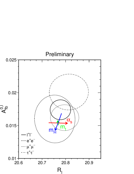
Figure 6: Contours of 68% probability in the $R_{\ell}$-$A^{0,\,\ell}_{\rm{FB}}$ plane. The Standard Model prediction for $m_{\mathrm{Z}}=91.1863$ GeV/c², $m_{\mathrm{t}}=175$ GeV/c², $m_{\mathrm{H}}=300$ GeV/c², and $\alpha_{s}=0.123$ is also shown. The lines with arrows correspond to the variation of the Standard Model prediction when $m_{\mathrm{t}}$, $m_{\mathrm{H}}$ or $\alpha_{s}(m_{\mathrm{Z}}^{2})$ are varied in the intervals $m_{\mathrm{t}}=175\pm 6$ GeV/c², $m_{\mathrm{H}}=300^{+700}_{-240}$ GeV/c², and $\alpha_{s}(m_{\mathrm{Z}}^{2})=0.123\pm 0.006$, respectively. The arrows point in the direction of increasing values of $m_{\mathrm{t}}$, $m_{\mathrm{H}}$ and $\alpha_{s}$.

The results of the five parameter fit can be used to derive the leptonic and hadronic partial decay widths of the $Z$ boson. An important aspect of these measurements is the information relayed regarding the invisible $Z$ decay width, given by

$$\Gamma_{\mathrm{inv}}\,=\,\Gamma_{\mathrm{Z}}\,-\,\Gamma_{\mathrm{had}}\,-\,(3+\delta_{\tau})\,\Gamma_{\ell\ell}\ .$$

Here $\delta_{\tau}=-0.0023$ represents a small correction due to the $\tau$-mass. The measurements give $\Gamma_{\mathrm{inv}}/\Gamma_{\ell\ell}=5.952\pm 0.023$. The Standard Model predicts $\Gamma_{\nu\nu}/\Gamma_{\ell\ell}=1.991\pm 0.001$, giving for the number of light neutrino species

$$N_{\nu}\,=\,{\Gamma_{\mathrm{inv}}\over\Gamma_{\ell\ell}}\,\left({\Gamma_{\ell\ell}\over\Gamma_{\nu\nu}}\right)\,=\,2.989\pm 0.012\ .$$

The advantage here is again the use of ratios. The partial widths have a non-negligible top mass dependence due to radiative corrections. Since these corrections are mostly universal, the dependence is significantly reduced in the ratio of partial widths. The disadvantage is that the result for the number of light neutrino species is only valid in the framework of the Standard Model.

2.4 Polarization

The Standard Model predicts parity violation not only for charged currents but for neutral currents as well. For the process $\mbox{$e^{+}e^{-}$}\rightarrow\mbox{$f\overline{f}$ }$ it manifests itself through a difference in production cross section for fermions with a different polarization. Polarization studies have experimentally been approached in two ways. One method, employed by the SLC collider, is to polarize the electron beam and measure the asymmetry $A_{\rm{LR}}$ defined as

$$\mbox{$A_{\rm{LR}}$}\,=\,{\sigma_{\rm L}\,-\,\sigma_{\rm R}\over\sigma_{tot}}$$

where $\sigma_{R(L)}$ is the total production cross section for right (left) handed polarized electrons. The source of polarized electrons is a strained GaAs photocathode, illuminated with circularly polarized light. Because of the mechanical strain in the solid there is no theoretical limitation to the polarization achievable. The SLC polarization group has steadily improved the polarization over the years reaching an average polarization during the 1994-1995 run of ${\cal P}_{e}=(77.34\pm 0.62)\%$. The degree of polarization is measured using a multi-channel Čerenkov detector which measures Compton-scattered electrons from the collision of the longitudinally polarized electron beam with a circularly polarized photon beam. The laser polarization can be flipped randomly and the asymmetry in cross section is measured. Special care has been taken to determine the true luminosity weighted polarization for $Z$ production at the interaction point. The Compton polarimeter measures the polarization of the entire electron bunch. The machine optics and the inherent beam spread in the bunch, however, reduce the contribution from off-energy electrons to the $Z$ production luminosity [18]. These effects have all been evaluated and result in a small correction of $\sim$0.07% to the measured polarization. The uncertainty on the polarization measurement is dominated by the uncertainty on the calibration of the Čerenkov detector.

The measurement of $A_{\rm{LR}}$ is relatively straightforward, since it essentially relies on counting $Z$ events irrespective of their final state. The measurement is therefore relatively free of systematic effects. Events from the process $\mbox{$e^{+}e^{-}$}\rightarrow\mbox{$e^{+}e^{-}$}$ are excluded due to the large zero asymmetry contribution from the $t$-channel diagram. At the $Z$ pole, ignoring photonic corrections, $\mbox{$A_{\rm{LR}}$}=\mbox{$\cal A_{\rm e}$}$ independent of the final state couplings. The SLD collaboration measures [19]

$$\mbox{$A_{\rm{LR}}^{0}$}\,=\,0.1542\pm 0.0037\ .$$

where the superscript “0” indicates that small corrections have been applied, using the Standard Model dependencies, to correct for electroweak interference and pure photon exchange contributions. This result yields directly

$$\sin^{2}\!\theta_{\rm{eff}}^{\rm{lept}}\,=\,0.23061\pm 0.00047\ .$$

It is noteworthy that this single measurement has an accuracy similar to the measurement of $\sin^{2}\!\theta_{\rm{eff}}^{\rm{lept}}$ from $A^{0,\,\ell}_{\rm{FB}}$ from all LEP experiments combined. The sensitivities are related as ${\partial A_{\mathrm{FB}}\over\partial\sin^{2}\!\theta_{\rm{eff}}^{\rm{lept}}}={3\over 2}\mbox{$\cal A_{\rm f}$}{1\over{\cal P}_{e}}{\partial\mbox{$A_{\rm{LR}}$}\over\partial\sin^{2}\!\theta_{\rm{eff}}^{\rm{lept}}}$. Compared to an $A_{\rm{LR}}$ measurement using all $Z$ decay channels, an approximately 90-fold larger data sample is required to achieve a similar accuracy in $\sin^{2}\!\theta_{\rm{eff}}^{\rm{lept}}$ from $A_{\mathrm{FB}}$ using leptonic $Z$ decays.

The time-reversal of this process is measured at LEP where the polarization of the final state particles is measured for unpolarized $e^{+}e^{-}$-beams:

$${\cal P}_{f}\,=\,{\sigma_{R}^{f}\,-\,\sigma_{L}^{f}\over\sigma_{tot}}\,=\,\mbox{$\cal A_{\rm f}$}\ ,$$

where $\sigma_{R}^{f}$ ($\sigma_{L}^{f}$) refers to the production cross section for right(left)-handed fermions. Similarly to $A_{\rm{LR}}$ being independent of the final state couplings, the average polarization of the final state fermions is independent of the initial state couplings. Because of the helicity of fermions, ${\cal P}_{f}$ obviously has an angular dependence given by

$${\cal P}_{f}(\cos\vartheta) = -{{\cal A}_{\rm f}(1+\cos^{2}\vartheta)\,+\,2{\cal A}_{e}\,\cos\vartheta\over 1+\cos^{2}\vartheta\,+\,2{\cal A}_{e}{\cal A}_{\rm f}\cos\vartheta}\ .$$

This gives rise to a forward-backward polarization asymmetry

$$A_{\rm{FB}}^{{\cal P}_{f}}\, = \,{(\sigma_{L}^{f}-\sigma_{R}^{f})_{\rm F}\,-\,(\sigma_{L}^{f}-\sigma_{R}^{f})_{\rm B}\over(\sigma_{L}^{f}+\sigma_{R}^{f})_{\rm F}\,+\,(\sigma_{L}^{f}+\sigma_{R}^{f})_{\rm B}}$$

$$= \,{3\over 4}\,\mbox{$\cal A_{\rm e}$}\,=\,{3\over 4}\,\langle{\cal P}_{Z}\rangle\ ,$$

which obviously is independent of the final state couplings. The forward-backward asymmetry of the fermion polarization is governed by the average polarization of the $Z$ boson, $\langle{\cal P}_{Z}\rangle$, which depends only on the initial state couplings. The angular distribution of the polarization thus gives independent measurements of $\cal A_{\rm f}$ and $\cal A_{\rm e}$, linear in both variables, which allows a relative sign determination of $g_{V}$ and $g_{A}$.

The polarization has to date only been measured for $\tau$ leptons for which the decay products can be used as spin analyzers assuming the $V-A$ structure of the weak decay. The decays used are $\tau\rightarrow\pi\nu_{\tau}$, $\tau\rightarrow\rho\nu_{\tau}$, $\tau\rightarrow a_{1}\nu_{\tau}$, $\tau\rightarrow e\nu_{\tau}\nu_{e}$ and $\tau\rightarrow\mu\nu_{\tau}\nu_{\mu}$. The extraction of the $\tau$ polarization basically employs the particle momentum spectrum of the decay particles. The $\rho\nu_{\tau}$ and $\pi\nu_{\tau}$ decays contribute most significantly. The LEP measured average values for $\cal A_{\tau}$ and $\cal A_{\rm e}$,

$$\cal A_{\tau} = 0.1401\pm 0.0067$$

$$\cal A_{\rm e} = 0.1382\pm 0.0076\,,$$

are compatible with lepton universality. Assuming $\mathrm{e}-\tau$ universality, the values for $\cal A_{\tau}$ and $\cal A_{\rm e}$ can be combined giving $\mbox{$\cal A_{\ell}$}=0.1393\pm 0.0050$ .

2.5 Results on Neutral Current Couplings from the Lepton Sector

It is useful at this point to take stock of all the measurements in hand. The results on $\Gamma_{\ell\ell}$ from the line shape measurements, $A^{0,\,\ell}_{\rm{FB}}$, $\cal P_{\tau}$, $A_{\rm{FB}}^{\cal P_{\tau}}$ and $A_{\rm{LR}}$ are all proportional to $\cal A_{\ell}$ or a combination of $\cal A_{\ell}$’s. The results can be combined to determine the effective vector and axial-vector coupling constants for $e$, $\mu$ and $\tau$ and provides a test of lepton universality. Figure 7 summarizes the results as contours of 68% probability in the $g_{V}^{\ell}$-$g_{A}^{\ell}$ plane from LEP measurements. The solid contour results from a fit assuming lepton universality. Also shown is the one standard deviation band resulting from the $A_{\rm{LR}}$ measurement of SLD. The grid corresponds to the Standard Model prediction for $m_{\mathrm{t}}=175\pm 6$ GeV/c² and $m_{\mathrm{H}}=300^{+700}_{-240}$ GeV/c². The arrows point, as usual, in the direction of increasing value of $m_{\mathrm{t}}$ and $m_{\mathrm{H}}$. The average central values are given in Table 4. The neutrino coupling to the $Z$ is derived from the measured value of its invisible width, $\Gamma_{\mathrm{inv}}$, attributing it exclusively to the decay into three identical neutrino generations ($\Gamma_{\mathrm{inv}}=3\Gamma_{\nu\nu}$) and assuming $g_{A}^{\nu}=g_{V}^{\nu}=g_{\nu}$.

	LEP	LEP+SLD
$g_{V}^{\ell}$	$-0.03688\pm 0.00085$	$-0.03776\pm 0.00062$
$g_{A}^{\ell}$	$-0.50115\pm 0.00034$	$-0.50108\pm 0.00034$
$g_{\nu}$	$+0.5009\pm 0.0010$	$+0.5009\pm 0.0010$

Table 4: Results for the effective vector and axial-vector couplings from the combined LEP data assuming lepton universality. For the right column the SLD measurement of $A_{\rm{LR}}$ has been included.

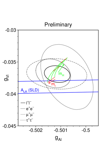
Figure 7: Contours of 68% probability in the $g_{V}^{\ell}$-$g_{A}^{\ell}$ plane from LEP measurements. The grid corresponds to the Standard Model prediction for $m_{\mathrm{t}}=175\pm 6$ GeV/c² and $m_{\mathrm{H}}=300^{+700}_{-240}$ GeV/c².

3 Heavy Flavor Sector

Of particular interest in the heavy flavor sector are the ratios of the $b$ and $c$ quark partial widths of the $Z$ to the total hadronic partial width, $R_{\mathrm{b}}\equiv\Gamma_{\mathrm{b\bar{b}}}/\Gamma_{\mathrm{had}}$ and $R_{\mathrm{c}}\equiv\Gamma_{\mathrm{c\bar{c}}}/\Gamma_{\mathrm{had}}$, respectively. Because the $b$ quark is in the same isospin doublet as the $t$ quark, the $Z\rightarrow\mbox{$b\overline{b}$}$ partial width receives vertex corrections which are unique to this particular decay mode and is thus very sensitive to physics beyond the Standard Model. For a long time both $R_{\mathrm{c}}$ and $R_{\mathrm{b}}$ deviated substantially from the Standard Model prediction. At the 1995 summer conferences the values reported were $R_{\mathrm{c}}$ = 0.1543 (74) and $R_{\mathrm{b}}$ = 0.2219 (17), compared to their Standard Model values of 0.1724 and 0.2156, respectively [20]. Taken at face value, assuming Gaussian errors, the $R_{\mathrm{b}}$ measurement ruled out the Standard Model at more than 99.9% CL, and excited tremendous interest among theorists proposing all kinds of extensions to the Standard Model [21]. Because the new results for $R_{\mathrm{b}}$ and $R_{\mathrm{c}}$ have changed significantly, the focus of this section will be on the new measurements of these two quantities.

3.1 $R_{\mathrm{c}}$

The $R_{\mathrm{c}}$ and $R_{\mathrm{b}}$ analyses rely on the identification of events as originating from the decay of a $c$ or $b$ quark, called “tagging”, with a minimal background and small hemisphere correlations. The oldest method to tag events employs the lepton $p_{T}$ spectrum of the semi-leptonic decays of the heavy quarks. Two new methods to tag $c$ quark events for the $R_{\mathrm{c}}$ measurement have been developed based on “charm counting” and tagging charm events using a “slow” pion.

The charm counting method is based on the observation that all charm quarks end up in the weakly decaying charmed hadrons ${\rm D}^{0}$, ${\rm D}^{+}$, ${\rm{D_{s}}}$ and ${\rm{\Lambda_{c}}}$:

$${\rm P}(c\rightarrow{\rm D}^{0})\,+\,{\rm P}(c\rightarrow{\rm D}^{+})\,+\,{\rm P}(c\rightarrow{\rm{D_{s}}})\,+\,$$

$${\rm P}(c\rightarrow{\rm{\Lambda_{c}}})(1\,+\,S_{\rm baryon})\,=\,1$$

Here ${\rm P}(c\rightarrow{\rm X}_{c})$ is the probability that a primary $c$ quark results in the production of charmed hadron ${\rm X}_{c}$. $S_{\rm baryon}$ is a correction factor of 0.15 for the formation of strange-charmed baryons, like $\Xi^{+}_{c}$. The charmed hadrons are reconstructed in the decay modes

${\rm D}^{0}$	$\rightarrow$	${\rm K}^{-}\pi^{+}$
${\rm D}^{+}$	$\rightarrow$	${\rm K}^{-}\pi^{+}\pi^{+}$
${\rm{D_{s}}}$	$\rightarrow$	$\phi\pi^{+}$
${\rm{D_{s}}}$	$\rightarrow$	${{\overline{\rm K}}^{*}}^{0}{\rm K}^{+}$
${\rm{\Lambda_{c}}}$	$\rightarrow$	${\rm pK}^{-}\pi^{+}$

Figure 8 shows the mass distributions from the OPAL experiment for the five decay modes [22]. These event samples are certainly not free of charmed hadrons from $b$ decays. The relatively large $b$ hadron lifetimes and hard $b$ fragmentation result in significantly longer apparent decay lengths and softer energy spectra for these charmed hadrons compared to those from primary charm production. This provides handles to separate the contributions from $b$ hadron decays and from prompt production. The overall contribution from $b$ decays in the event sample, however, still exceeds that from primary $c$ decays and the results are sensitive to uncertainties in $b$ fragmentation and $b$ hadron lifetimes. These are the dominant systematic uncertainties and have been addressed by Monte Carlo. The reconstruction efficiencies for each of the separate decays have also been determined by Monte Carlo. They are slightly lower for primary charmed hadrons than for charmed hadrons coming from $b$ decays. An important additional source of background is the production of charmed hadrons through gluon splitting, $g\rightarrow c{\overline{c}}$. Although the event selection is geared towards selecting energetic D mesons, about half of all the D mesons from gluon splitting remain in the event sample. The mean multiplicity of $c{\overline{c}}$ production from gluon splitting in hadronic $Z$ decays was measured from the production of ${\rm D}^{*}$ mesons to be ${\overline{n}}_{g\rightarrow c{\overline{c}}}=(4.4\pm 2.1)\%$ [23]. Recent measurements based on leptonic events yield ${\overline{n}}_{g\rightarrow c{\overline{c}}}=(2.38\pm 0.48)\%$, thus raising $R_{\mathrm{c}}$ since less charm background from gluon splitting is subtracted.

Figure 8: OPAL mass distributions of the five reconstructed D meson decays.

Knowing the efficiencies and the background contributions the data allows for a direct measurement of ${\Gamma_{\mathrm{c\bar{c}}}\over\Gamma_{\mathrm{had}}}\cdot{\rm P}(c\rightarrow{\rm X}_{c})\cdot BR_{{\rm X}_{c}}$. With the constraint that the probabilities for the weakly decaying charmed hadrons add up to one, the sum of these measurements, corrected for the decay branching ratios as listed by the particle data group, yields $R_{\mathrm{c}}$. It is important to note that no assumptions need to be made on the production rates of the individual charmed mesons. The analyses do depend, however, on the measured branching ratios, which are used as an external input. Because of a new measurement by ARGUS [24], the average branching ratio $BR({\rm D}^{0}\rightarrow{\rm K}^{-}\pi^{+})$ has changed significantly from (4.01$\pm$0.14)% to (3.83$\pm$0.12)% [25], also resulting in an increase in $R_{\mathrm{c}}$.

Alternative methods to measure $R_{\mathrm{c}}$ use the decay ${\rm D}^{*}\rightarrow{\rm D}^{0}\pi^{+}\rightarrow({\rm K}^{-}\pi^{+})\pi^{+}$. Because of the very low $Q$ value of the decay, the pion from the ${\rm D}^{*}$ decay has a very low $p_{T}$ with respect to the ${\rm D}^{*}$ line of flight and can be used to tag the event. The slow pion tag analyses generally proceed by first measuring the production rate of single tagged, exclusive ${\rm D}^{*}$ decays, $N_{d}$, given by

$${N_{d}\over N_{had}} \sim R_{\mathrm{c}}\cdot P(c\rightarrow{\rm D}^{*+})BR({\rm D}^{*+})\ \epsilon_{{\rm D}^{*+}}$$

where $N_{had}$ is the number of hadronic $Z$ decays, and $\epsilon_{{\rm D}^{*+}}$ the ${\rm D}^{*+}$ reconstruction efficiency. In a second step an inclusive “slow” pion tag is applied to the opposite hemisphere giving for the number of double tagged events, $N_{dd}$,

$${N_{dd}\over N_{had}} \sim R_{\mathrm{c}}\cdot\left[P(c\rightarrow{\rm D}^{*+})BR({\rm D}^{*+})\right]^{2}\,\epsilon_{{\rm D}^{*+}}\,\epsilon_{s}$$

with $\epsilon_{s}$ the slow pion tag efficiency. Each experiment has its own variant of this procedure. DELPHI, for example, uses a fully inclusive tag, with high efficiency and large backgrounds [26]. ALEPH [27] and OPAL [28] use an inclusive–exclusive tag using ${\rm D}^{*}$ mesons, although ALEPH has also tried a fully exclusive tag of D-meson decays with reduced statistics but much higher purity. An important bonus of these analyses is that $\mathrm{P(c\rightarrow D^{*+})\times BR(D^{*+}\rightarrow\pi^{+}D^{0})}$ is measured directly and does not need to be taken from low-energy data as external input. A summary of all $R_{\mathrm{c}}$ results from the different measurement techniques is shown in Fig. 9.

To summarize, the main reasons for the increase in $R_{\mathrm{c}}$ are: i) more data analysed, ii) decrease in the gluon splitting probability $g\rightarrow c{\overline{c}}$, iii) decrease in the branching ratio $BR({\rm D}^{0}\rightarrow{\rm K}^{-}\pi^{+})$ and iv) new Aleph measurement. The new value of $R_{\mathrm{c}}$ is in excellent agreement with the Standard Model prediction. The change is dominated by the updated OPAL measurement and the new ALEPH result.

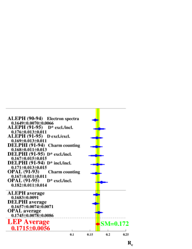
Figure 9: Summary of $R_{\mathrm{c}}$ measurements.

3.2 $R_{\mathrm{b}}$

The measurements of $R_{\mathrm{b}}$ also employ the single-tag and double-tag technique. As noted in the measurement of $R_{\mathrm{c}}$, in the single tag method the number of tagged events is counted. This number is corrected for backgrounds from other flavors and for the tagging efficiency to calculate the true fraction of hadronic $Z$ decays of that flavor. For the double-tag measurement, the event is divided into two hemispheres and both hemispheres are tagged. Writing the number of tagged single hemispheres as $N_{t}$, the number of events with both hemispheres tagged as $N_{tt}$, then for a total of $N_{\rm{had}}$ hadronic $Z$ decays the measurement of $R_{\mathrm{b}}$ follows from

$$\frac{N_{t}}{2N_{\rm{had}}} = \varepsilon_{b}R_{\mathrm{b}}+\varepsilon_{c}R_{\mathrm{c}}+\varepsilon_{uds}(1-R_{\mathrm{b}}-R_{\mathrm{c}}),$$

$$\frac{N_{tt}}{N_{\rm{had}}} = (1+\rho_{b})\varepsilon_{b}^{2}R_{\mathrm{b}}+\varepsilon_{c}^{2}R_{\mathrm{c}}+$$ (1)

$$\varepsilon_{uds}^{2}(1-R_{\mathrm{b}}-R_{\mathrm{c}}),$$

where $\varepsilon_{b}$, $\varepsilon_{c}$ and $\varepsilon_{uds}$ are the tagging efficiencies per hemisphere for $b$, $c$ and light-quark events, and $\rho_{b}$ accounts for the fact that the tagging efficiencies between the hemispheres may be correlated. By measuring both the single and double tag rate, the $b$ tagging efficiency can be determined directly from the data, reducing the systematic uncertainties in the measurement.

The most precise determinations of $R_{\mathrm{b}}$ use the lifetime tag of the $b$-quark. Events are tagged by reconstructing either a secondary vertex (SV) or an impact parameter. Events originating from $b$ decays will have large positive values for these quantities. The negative tails in these distributions are used to measure the resolutions and control systematic effects. The measurements of $R_{\mathrm{b}}$ were, and still are, systematics dominated. Two of the dominant sources of systematics are the charm background and the hemisphere correlations. The experimental effort therefore has gone into reducing both $\varepsilon_{c}$ and $\rho_{b}$ in equation (1). It should be pointed out here that the correlations are analysis dependent and are very different for an impact parameter analysis compared to a measurement using the SV technique.

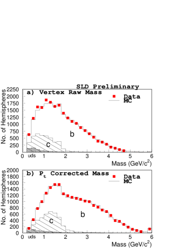
Figure 10: a) Secondary vertex mass distribution as measured by SLD (points) together with $u,d,s$ (cross hatched) and charm (hatched) background contributions. b) Mass distribution corrected for missing transverse energy.

As for the charm sector, there have been two significant developments. First of all, charm decays are currently much better understood by the LEP and SLD experiments. The production rates of the different charmed mesons and the branching ratios of cascade decays, for example, are now measured by the experiments themselves. Secondly, a new lifetime and mass tag, first presented by SLD [29] with a similar method developed independently by ALEPH, has allowed for a substantial reduction of the charm background in the data sample. This tag proceeds by first computing the confidence level that all tracks in a hemisphere come from the primary vertex (PV). Tracks least consistent with the PV are then combined and their invariant mass calculated. Figure 10a show this mass spectrum as measured by SLD. A cut is placed at approximately the charm threshold to obtain the $b$ rich sample. Since the interaction point is very well known at SLC, the SLD experiment can take this method one step further and correct for the undetected neutrals in the $b$ decay. A correction is applied to correct for the missing energy transverse to the direction of flight of the $b$ hadron, as given by the PV and SV (Fig. 10b). A cut on this “$p_{T}$ corrected vertex mass” is applied to further enrich the sample. Due to the larger spread in beam size at LEP, this correction cannot be applied by the LEP experiments. Note that the presence of charm background in the sample gives rise to an explicit correlation between $R_{\mathrm{b}}$ and $R_{\mathrm{c}}$. Figure 11 summarizes the $b$ tagging performance of the different experiments. They all reach an impressive purity with good detection efficiencies.

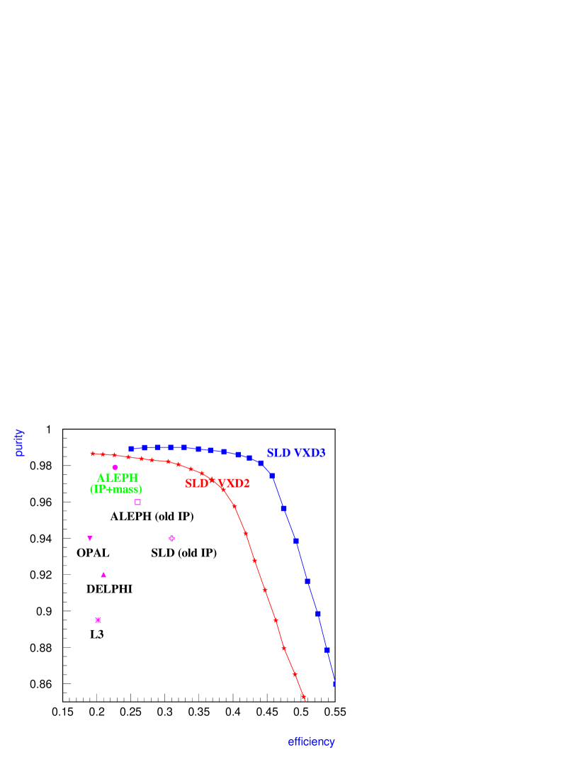
Figure 11: $b$ tag performance per hemisphere for the different experiments.

There has also been considerable progress in the understanding of hemisphere correlations. These correlations arise mainly from the primary vertex, and from detector and QCD effects. If, for example, one $b$ hadron has a very long lifetime, the efficiency for tagging the other $b$ will be decreased due to the degraded PV resolution. As most $b$ hadrons are roughly back to back, detector correlations are introduced if a region of poorer instrumentation is hit. The ALEPH experiment has switched to a method where a PV is calculated for each hemisphere, thereby eliminating one of the dominant contributions to $\rho_{b}$. An alternative method, pioneered by DELPHI, employs multiple mutually exclusive tags using the lifetime-mass information as well as event shape variables. The determination of the correlations and their effect on the measurement is complicated. They are evaluated using both data and Monte Carlo. It are these correlations as well as the residual background of other flavors which are still the main sources of systematic uncertainty. A new ALEPH measurement, using the full 91–95 statistics, has currently the smallest error of all individual measurements. It is based on multiple mutually exclusive tags using event shape and lifetime-mass information and gives $R_{\mathrm{b}}=0.2158\pm 0.0009\pm 0011$, using the Standard Model value for $R_{\mathrm{c}}$ [30]. In addition to this new measurement, DELPHI has updated its measurements by inclusion of the 1994 data [26] and L3 has for the first time presented a lifetime tag measurement [31]. All results are summarized in Fig. 12. The combined LEP/SLD average is $R_{\mathrm{b}}=0.2178\pm 0011$ ($R_{\mathrm{c}}=0.172$) to be compared to the Standard Model prediction of $R_{\mathrm{b}}=0.2158$ .

In summary, the main reasons for the decrease in $R_{\mathrm{b}}$ are: i) inclusion of much more data, ii) better understanding of the charm sector, iii) reduction of the charm background and iv) a better understanding of the hemisphere correlations. All effects have the tendency to lower $R_{\mathrm{b}}$, though the change is dominated by inclusion of new data. The change in external input parameters results in a change in $R_{\mathrm{b}}$ of only 0.0003 .

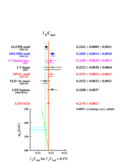
Figure 12: Summary of $R_{\mathrm{b}}$ measurements.

3.3 Other Heavy Flavor Results.

The measurements in the heavy flavor sector encompass many other results. The forward-backward asymmetries for $b$ and $c$ quarks measured on- and off-pole, the semi-leptonic branching ratios $BR(\mbox{$b{\mathrm{\rightarrow}\ell X}$})$, $BR(\mbox{$c{\mathrm{\rightarrow}\ell X}$})$, the average $b\overline{b}$ mixing parameter $\chi$, the various production probabilities for D-mesons and the quark coupling parameters $\cal A_{\rm b}$ and $\cal A_{\rm c}$ are all measured. The latter two are measured directly by SLD from the polarized forward-backward asymmetry:

$$A_{\rm{FB}}^{\rm{pol}(f)} = {(\sigma_{L}^{f}-\sigma_{R}^{f})_{\rm F}\,-\,(\sigma_{L}^{f}-\sigma_{R}^{f})_{\rm B}\over(\sigma_{L}^{f}+\sigma_{R}^{f})_{\rm F}\,+\,(\sigma_{L}^{f}+\sigma_{R}^{f})_{\rm B}}\,=\,{3\over 4}\,\mbox{$\cal A_{\rm f}$}\ .$$

Three different techniques are used to measure $\cal A_{\rm b}$ based on the determination of the jet-charge, tagging events through their lepton $p_{T}$ spectrum and tagging with K^± mesons [32]. These analyses have similar sources of systematic error compared to the LEP asymmetry measurements. The SLD measurements yield

$$\cal A_{\rm b} = 0.863\pm 0.049$$

$$\cal A_{\rm c} = 0.625\pm 0.084\ .$$

All in all, 17 variables are measured in the heavy flavor sector. This set is reduced by four by shifting the off-pole forward-backward asymmetries to the pole center of mass energy. In a fashion similar to the results from the lepton sector, the averages of all measurements have been determined taking into account their correlations [33].

4 Combining All Results

It is widely anticipated that the Standard Model is just an approximate theory and should eventually be replaced by a more complete and fundamental description of the underlying forces in nature. The individual measurements probe different aspects of the Standard Model and all measurements combined provide a powerful constraint. To test how well the Standard Model fares one first determines how well the individual measurements can be accommodated within its framework. If they are all consistent, the measurements can be combined to provide constraints on those parameters that enter via radiative corrections. These constraints can then be compared with direct measurements, if they exist. This can be an iterative process in which more and more measurements are included in the full set of electroweak measurements in each subsequent step. In the following subsections the results of taking these successive steps will be described.

4.1 The Effective Electroweak Mixing Angle $\sin^{2}\!\theta_{\rm{eff}}^{\rm{lept}}$

In section 2.5 the results on $\Gamma_{\ell\ell}$, $A^{0,\,\ell}_{\rm{FB}}$, $\cal P_{\tau}$, $A_{\rm{FB}}^{\cal P_{\tau}}$ and $A_{\rm{LR}}$ were combined to determine the effective vector and axial-vector coupling constants. All asymmetry measurements can be combined into a single observable, the effective electroweak mixing angle. For a combined average of $\sin^{2}\!\theta_{\rm{eff}}^{\rm{lept}}$ from $A^{0,\,\ell}_{\rm{FB}}$, $\cal A_{\tau}$, $\cal A_{\rm e}$ and $A_{\rm{LR}}$ only the assumption of lepton universality, already inherent in the definition of $\sin^{2}\!\theta_{\rm{eff}}^{\rm{lept}}$, is needed. Also the quark forward-backward asymmetries, $A^{0,\,b}_{\rm{FB}}$ and $A^{0,\,c}_{\rm{FB}}$, and the forward-backward asymmetry in mean jet charge, $\langle\mbox{Q}_{\mbox{FB}}\rangle$, are included in this average, as these asymmetries have a reduced sensitivity to corrections particular to the hadronic vertex. Figure 13 shows the comparison of the individual measurements with the Standard Model prediction. It is seen that there is good agreement between the average of $\sin^{2}\!\theta_{\rm{eff}}^{\rm{lept}}=0.23165\pm 0.00024$, a 0.1% measurement, with the Standard Model prediction of $\sin^{2}\!\theta_{\rm{eff}}^{\rm{lept}}=0.23167$. It should be noted that the SLD value for $\sin^{2}\!\theta_{\rm{eff}}^{\rm{lept}}$ from $A_{\rm{LR}}$ is 2.2 standard deviations low compared to the world average. Most of that discrepancy comes from the early SLD data.

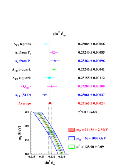
Figure 13: Summary of $\sin^{2}\!\theta_{\rm{eff}}^{\rm{lept}}$ measurements from the forward-backward asymmetries of leptons, $\tau$ polarization, inclusive quarks, heavy quark asymmetry and the SLD polarization asymmetry.

		Measurement with	Standard	Pull
		Total Error	Model
a)	LEP
	line-shape and
	lepton asymmetries:
	$m_{\mathrm{Z}}$ [GeV/c2]	$91.1863\pm 0.0020\phantom{0}$	91.1861	$0.1$
	$\Gamma_{\mathrm{Z}}$ [GeV]	$2.4946\pm 0.0027\phantom{0}$	2.4960	$-0.5$
	$\sigma_{\mathrm{h}}^{0}$ [nb]	$41.508\pm 0.056\phantom{00}$	41.465	$0.8$
	$R_{\ell}$	$20.778\pm 0.029\phantom{00}$	20.757	$0.7$
	$A^{0,\,\ell}_{\rm{FB}}$	$0.0174\pm 0.0010\phantom{0}$	0.0159	$1.4$
	+ correlation matrix
	$\tau$ polarization:
	$\cal A_{\tau}$	$0.1401\pm 0.0067\phantom{0}$	0.1458	$-0.9$
	$\cal A_{\rm e}$	$0.1382\pm 0.0076\phantom{0}$	0.1458	$-1.0$
	b and c quark results:
	$R_{\mathrm{b}}$	$0.2179\pm 0.0012\phantom{0}$	0.2158	$1.8$
	$R_{\mathrm{c}}$	$0.1715\pm 0.0056\phantom{0}$	0.1723	$-0.1$
	$A^{0,\,b}_{\rm{FB}}$	$0.0979\pm 0.0023\phantom{0}$	0.1022	$-1.8$
	$A^{0,\,c}_{\rm{FB}}$	$0.0733\pm 0.0049\phantom{0}$	0.0730	$0.1$
	+ correlation matrix
	$\mathrm{q}\overline{\mathrm{q}}$ charge asymmetry:
	$\sin^{2}\!\theta_{\rm{eff}}^{\rm{lept}}$ ($\langle\mbox{Q}_{\mbox{FB}}\rangle$)	$0.2320\pm 0.0010\phantom{0}$	0.23167	$0.3$
b)	SLD
	$\sin^{2}\!\theta_{\rm{eff}}^{\rm{lept}}$ ($A_{\rm{LR}}$)	$0.23061\pm 0.00047$	0.23167	$-2.2$
	$R_{\mathrm{b}}$	$0.2149\pm 0.0038\phantom{0}$	0.2158	$-0.2$
	$\cal A_{\rm b}$	$0.863\pm 0.049\phantom{00}$	0.935	$-1.4$
	$\cal A_{\rm c}$	$0.625\pm 0.084\phantom{00}$	0.667	$-0.5$
c)	$\overline{p}p$ and $\nu$N
	$m_{\mathrm{W}}$ [GeV/c2] ($\overline{p}p$ )	$80.356\pm 0.125\phantom{00}$	80.353	$0.3$
	$1-m_{\mathrm{W}}^{2}/m_{\mathrm{Z}}^{2}$ ($\nu$N)	$0.2244\pm 0.0042\phantom{0}$	0.2235	$0.2$
	$m_{\mathrm{t}}$ [GeV/c2] ($\overline{p}p$ )	$175\pm 6\phantom{00}\phantom{00}$	172	$0.5$

Table 5: Summary of measurements included in the combined analysis of Standard Model parameters. Section a) summarizes LEP averages, Section b) SLD results and Section c) electroweak measurements from $\overline{p}p$ colliders and $\nu$N scattering. The Standard Model results in column 3 and the difference between measurement and fit in units of the total measurement error in column 4 are derived from the Standard Model fit including all data with the Higgs mass treated as a free parameter.

4.2 The Coupling Parameters $\cal A_{\rm f}$

The (polarized) forward-backward asymmetry measurements all measure either the product of coupling parameters $\cal A_{\rm f}$ of different fermion species or the single coupling directly. Also the measurement of the $\tau$-polarization determines $\cal A_{\tau}$ and $\cal A_{\rm e}$, separately. Assuming lepton universality, $\cal A_{\ell}$ as determined from $A^{0,\,\ell}_{\rm{FB}}$, $\mbox{$\cal P_{\tau}$}(\cos\vartheta)$ and $A_{\rm{LR}}$ is

$$\cal A_{\ell} = 0.1466\pm 0.0033\qquad{\rm(LEP)}$$

$$\cal A_{\ell} = 0.1500\pm 0.0025\qquad{\rm(LEP+SLD)}$$

Note that $\cal A_{\ell}$ is pushed up by one standard deviation by inclusion of the SLD $A_{\rm{LR}}$ measurement. Using these values for $\cal A_{\rm f}$ the couplings for the heavy flavors can be determined from $A^{0,\,b}_{\rm{FB}}$ and $A^{0,\,c}_{\rm{FB}}$ and the heavy flavor left-right asymmetries from SLD. Taking the LEP average for $\cal A_{\rm f}$ gives

$$\cal A_{\rm b} = 0.890\pm 0.029$$

$$\cal A_{\rm c} = 0.667\pm 0.047$$

whereas using the combined LEP/SLD result for $\cal A_{\rm f}$ gives

$$\cal A_{\rm b} = 0.867\pm 0.022$$

$$\cal A_{\rm c} = 0.649\pm 0.040\ ,$$

moving $\cal A_{\rm b}$ down by about one standard deviation. $\cal A_{\rm c}$ agrees very well with the Standard Model prediction of 0.667. The world average value for $\cal A_{\rm b}$, however, deviates by 3.1 standard deviations from the Standard Model prediction of 0.935. This deviation is not without controversy. It should be kept in mind that the value for $\cal A_{\rm b}$ as obtained above is not an independent measurement since it uses the value for $\cal A_{\rm e}$. Fluctuations in the measurement of $\cal A_{\rm e}$, a measurement which is unrelated to the b-coupling per se, increase the deviation of $\cal A_{\rm b}$ with the Standard Model prediction. There is only one direct measurement of $\cal A_{\rm b}$, namely from the left-right forward-backward asymmetry measurement by SLD, $\mbox{$\cal A_{\rm b}$}=0.863\pm 0.049$, which is 1.4 standard deviations low compared to the Standard Model value. If one wishes to combine different measurements a value less prone to fluctuations in other measurements may be obtained by using the Standard Model prediction for $\cal A_{\rm e}$.

4.3 Constraints on the Standard Model

The full set of observables can be fit within the framework of the Standard Model to up-to-date theoretical calculations [34] and an estimate of the free parameters of the model can be obtained along with the Standard Model prediction for each observable. The accuracy of the measurements makes them sensitive to higher order electroweak radiative corrections. The leading corrections are due to propagator and vertex effects which introduce a dependence of the observables on $m_{t}$ (quadratically) and $m_{\mathrm{H}}$ (logarithmically). Table 5 summarizes the averages of the various measurements from LEP (section a), from SLD (section b), and from electroweak measurements from $\overline{p}p$ collider and $\nu$N scattering experiments (section c). The third column tabulates the Standard Model predictions and the last column lists the differences between measurement and fit in units of the total measurement error. In the Standard Model fit the Higgs mass has been treated, for the first time, as a free parameter. Given the multitude of measurements, there is good agreement with the theoretical predictions. It seems that the only modest deviations lie within the third family: $A^{0,\,\tau}_{\rm{FB}}$, which 2.3 standard deviations high, $A^{0,\,b}_{\rm{FB}}$, which is 1.8 standard deviations low, and $R_{\mathrm{b}}$ which has come down considerably from the earlier measurements but is still high by 1.8 standard deviations. Figures 14 and 15 give an overall picture of the comparison with the Standard Model in the leptonic and hadronic sector, respectively. Figure 14 shows a comparison with the Standard Model of $\Gamma_{\ell\ell}$ from LEP, and $\sin^{2}\!\theta_{\rm{eff}}^{\rm{lept}}$ from asymmetries measured at LEP and SLD. Good agreement with the Standard Model prediction is observed. The star indicates the prediction if among the electroweak radiative corrections only the photon vacuum polarization is included, showing evidence that the data is truly sensitive to electroweak corrections. The length of the arrow indicates the error on $\alpha(m_{\mathrm{Z}}^{2})$, which is as large as the error on $\sin^{2}\!\theta_{\rm{eff}}^{\rm{lept}}$ from LEP and SLD combined [35].

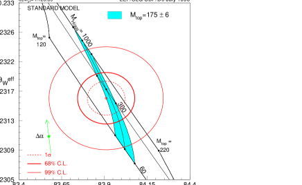
Figure 14: The LEP/SLD measurements of $\sin^{2}\!\theta_{\rm{eff}}^{\rm{lept}}$ and $\Gamma_{\ell\ell}$ and the Standard Model prediction. The shaded area is obtained when $m_{\mathrm{t}}$ is restricted to its measured mass range, $m_{\mathrm{t}}=175\pm 6$ GeV/c². The star shows the predictions if among the electroweak radiative corrections only the photon vacuum polarization is included. The corresponding arrow shows the variation of this prediction if $\alpha(m_{\mathrm{Z}}^{2})$ is changing by one standard deviation. This variation gives an additional uncertainty on the Standard Model prediction which is not indicated in the figure.

In Fig. 15 the fitted result for $R_{\mathrm{b}}$ with $R_{\mathrm{c}}$ fixed to its Standard Model value is plotted versus $\sin^{2}\!\theta_{\rm{eff}}^{\rm{lept}}$. If one assumes the Standard Model dependence of the partial widths on $\sin^{2}\!\theta_{\rm{eff}}^{\rm{lept}}$ for the light quarks and the $c$ quark, and takes $\alpha_{s}(m_{\mathrm{Z}}^{2})=0.123\pm 0.006$, $R_{\ell}$ imposes a constraint on the two variables, shown as the diagonal band. Good agreement is seen among these three experimentally independent measurements, showing the consistency of the LEP data.

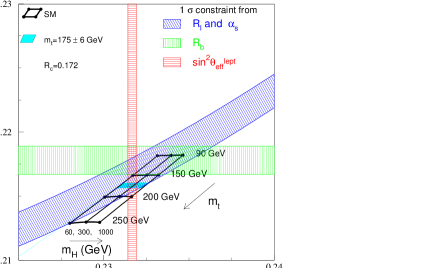
Figure 15: The LEP/SLD measurements of $\sin^{2}\!\theta_{\rm{eff}}^{\rm{lept}}$ and $R_{\mathrm{b}}(R_{\mathrm{c}}=0.172)$. The grid indicates the Standard Model prediction. Also shown is the constraint resulting from the measurement of $R_{\ell}$, assuming $\alpha_{s}(m_{\mathrm{Z}}^{2})=0.123\pm 0.006$, as well as the Standard Model dependence of light-quark partial widths on $\sin^{2}\!\theta_{\rm{eff}}^{\rm{lept}}$.

	LEP	LEP + SLD	LEP + SLD
			+ $\overline{p}p$ and $\nu$N data
$m_{\mathrm{t}}$ (GeV/c2)	$171\;\pm 8\;^{+17}_{-19}$	$177\;^{+7}_{-8}\;{}^{+17}_{-19}$	$177\pm 7\;^{+16}_{-19}$
$\alpha_{s}(m_{\mathrm{Z}}^{2})$	$0.122\pm 0.003\;\pm 0.002$	$0.121\pm 0.003\;\pm 0.002$	$0.121\pm 0.003\;\pm 0.002$
$\sin^{2}\!\theta_{\rm{eff}}^{\rm{lept}}$	$0.23209\pm 0.00024\;^{+0.00007}_{-0.00016}$	$0.23179\pm 0.00022\;^{+0.00006}_{-0.00013}$	$0.23179\pm 0.00020\;^{+0.00006}_{-0.00014}$
$1-m_{\mathrm{W}}^{2}/m_{\mathrm{Z}}^{2}$	$0.2247\pm 0.0009\;^{+0.0003}_{-0.0002}$	$0.2238\pm 0.0008\;^{+0.0004}_{-0.0002}$	$0.2238\pm 0.0008\;^{+0.0003}_{-0.0002}$
$m_{\mathrm{W}}$ (GeV/c2)	$80.292\pm 0.048\;^{+0.010}_{-0.018}$	$80.337\pm 0.041\;^{+0.010}_{-0.021}$	$80.338\pm 0.040\;^{+0.009}_{-0.018}$

Table 6: Results of fits to the three sets of electroweak precision data, as summarized in Table 5, for $m_{\mathrm{t}}$ and $\alpha_{s}(m_{\mathrm{Z}}^{2})$. The central values and the first errors quoted refer to $m_{\mathrm{H}}=300$ GeV/c². The second errors correspond to the variation of the central value when varying $m_{\mathrm{H}}$ in the interval $60<m_{\mathrm{H}}<1000$ GeV/c². The bottom part of the table lists derived results for $\sin^{2}\!\theta_{\rm{eff}}^{\rm{lept}}$, $1-m_{\mathrm{W}}^{2}/m_{\mathrm{Z}}^{2}$ and $m_{\mathrm{W}}$.

4.4 Predictive Power of the Standard Model

Having shown the consistency of all the measurements with the Standard Model, it is justified to combine them to determine the free parameters of the model. A beautiful precedent has been the prediction of the top quark mass. The top quark was discovered [36] in the mass region right were it was predicted to be. Table 6 shows the constraints on two free parameters of the Standard Model, $m_{\mathrm{t}}$ and $\alpha_{s}(m_{\mathrm{Z}}^{2})$, when fitting the measurements to Standard Model calculations. No external constraint on $\alpha_{s}(m_{\mathrm{Z}}^{2})$ has been imposed. The three columns present the results corresponding to the data sets as listed in Table 5 sections a, b and c, respectively. The central values and the first errors quoted refer to $m_{\mathrm{H}}=300$ GeV/c². The second errors correspond to the variation of the central value when varying $m_{\mathrm{H}}$ in the interval $60<m_{\mathrm{H}}<1000$ GeV/c². The bottom part of the table lists derived results for $\sin^{2}\!\theta_{\rm{eff}}^{\rm{lept}}$, $1-m_{\mathrm{W}}^{2}/m_{\mathrm{Z}}^{2}$ and $m_{\mathrm{W}}$. The first error includes the uncertainty on the fine structure constant $\alpha(m_{\mathrm{Z}}^{2})=1/(128.896\pm 0.090)$. This large uncertainty [35] is becoming a limiting factor in the predictive power of the Standard Model. It causes an uncertainty of 0.00023 on the prediction of $\sin^{2}\!\theta_{\rm{eff}}^{\rm{lept}}$, an uncertainty as large as the current experimental uncertainty, and an uncertainty of 4 GeV/c² on $m_{\mathrm{t}}$. Theoretical uncertainties due to missing higher order corrections, are neglected for the results presented in Tables 6 and 7. They are estimated [37] to be less than 1 GeV/c² on $m_{\mathrm{t}}$, less than 0.001 on $\alpha_{s}(m_{\mathrm{Z}}^{2})$ and 0.1 on $\log(m_{\mathrm{H}})$. Although the theoretical error on $\log(m_{\mathrm{H}})$ is still smaller than the experimental error, it is significantly larger than the theoretical error on $m_{\mathrm{t}}$ or $\alpha_{s}(m_{\mathrm{Z}}^{2})$. Increased precision in both the fine structure constant and the theoretical calculations is clearly warranted.

The fitted value of $m_{\mathrm{t}}$ is in excellent agreement with the measured top mass of $m_{\mathrm{t}}=175\pm 6$ GeV/c² [36]. Note that the precision of the direct top mass measurement has (finally) surpassed the indirect measurement. In the determination of the central value of $m_{\mathrm{t}}$, however, the mass of the Higgs boson has been fixed to 300 GeV/c². Since there is a strong correlation between the top and Higgs mass it should be possible to constrain $m_{\mathrm{H}}$, given the Tevatron direct measurements of $m_{\mathrm{t}}$. The result of the fit is shown in Table 7 and Fig. 16. The combination of the world’s data starts to constrain the Higgs mass and prefers a value of $m_{\mathrm{H}}=149^{+148}_{-82}$ GeV/c². The correlation between $m_{\mathrm{H}}$ and $m_{\mathrm{t}}$ is apparent. It should be noted that the correlation would even be larger if the $R_{\mathrm{b}}$ measurement is not used, as $R_{\mathrm{b}}$ is insensitive to $m_{\mathrm{H}}$. It should be pointed out that the central value of the preferred Higgs mass, with the corresponding error, can vary dramatically if one of the results is excluded from the fit. The overall constraint on $m_{\mathrm{H}}$ is therefore still rather weak. The implications of these results on new physics are discussed in [38].

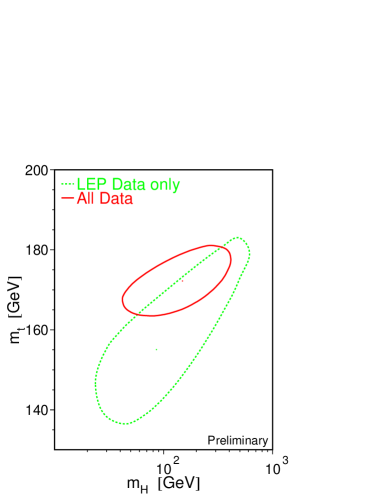
Figure 16: 68% confidence level contours in $m_{\mathrm{t}}$ and $m_{\mathrm{H}}$ when using as constraint LEP data only (dashed line) and the world’s data (solid line).

	LEP	LEP+SLD+$\overline{p}p$
		+$\nu$N data+$m_{\mathrm{t}}$
$m_{\mathrm{t}}$ [GeV/c2]	$155^{+18}_{-13}$	$172\pm 6$
$m_{\mathrm{H}}$ [GeV/c2]	$86^{+202}_{-51}$	$149^{+148}_{-82}$
$\log(m_{\mathrm{H}})$	$1.93^{+0.52}_{-0.39}$	$2.17^{+0.30}_{-0.35}$
$\alpha_{s}(m_{\mathrm{Z}}^{2})$	$0.121\pm 0.003$	$0.120\pm 0.003$

Table 7: Results for parameters in the Standard Model from fits to LEP data alone and to all data including the Tevatron top quark mass determination.

4.5 More on $W$ Properties

Recently the LEP center of mass energy has crossed the $W$ pair production threshold, allowing for a direct measurement of $W$ boson properties at LEP complementing the measurements at $\overline{p}p$ colliders. One of the more interesting measurements is the $W$ mass measurement. Given the strong sensitivity of the $WW$ production threshold to $m_{\mathrm{W}}$ a good precision is obtained with relatively few events by measuring the total production cross section at threshold. Given the nature of this measurement, the dominant uncertainties are obviously those on the luminosity and center of mass energy. All four LEP experiments have an initial measurement of the production cross section at ${\sqrt{s}}=161.3\pm 0.2$ GeV, listed in Table 8, resulting in a measurement of the $W$ mass of $m_{\mathrm{W}}=80.4\pm 0.3\pm 0.1$ GeV/c² (see Fig. 17) [39].

ALEPH	$4.9^{+1.9}_{-1.6}$ pb
DELPHI	$3.5^{+1.5}_{-1.3}$ pb
L3	$2.9^{+1.3}_{-1.1}$ pb
OPAL	$3.9^{+1.8}_{-1.4}$ pb
LEP average	$3.6\pm 0.7$ pb

Table 8: LEP measurements of the $W$ pair production cross section at ${\sqrt{s}}=161.3\pm 0.2$ GeV.

The Standard Model process of $W$-pair production is characterized by large cancellations between the $s$ and $t$ channel production processes. The contributions from the $t$ channel diagrams by themselves violate unitarity. The measurements of the pair production cross section are therefore a beautiful demonstration of the gauge cancellations in the Standard Model, as demonstrated already with the study of $W$ pairs produced at the $\overline{p}p$ colliders [40]. The direct production of $W$ bosons now also allows for a direct measurement of its magnetic dipole and electric quadrupole moment at LEP, two quantities on which stringent limits already exist from the $\overline{p}p$ experiments [41].

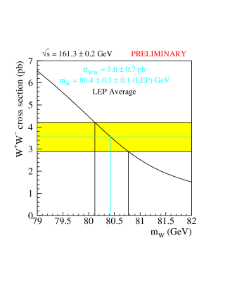
Figure 17: $W$ mass from the LEP average of the measurements of threshold $W$ pair production cross section at ${\sqrt{s}}=161.3\pm 0.2$ GeV.

5 Conclusions

It has been unprecedented that an anticipated quark was discovered with a mass exactly within the range predicted from loop corrections within a theoretical framework. This is a remarkable feat for experimentalists and theorists alike and attests to the enormous success of the Standard Model. Even though many measurements are now being carried out with excruciating precision, the Standard Model shows no signs of giving up its claim of being the description of the fundamental interactions as we know them. The large deviations that existed in the $R_{\mathrm{b}}$ and $R_{\mathrm{c}}$ measurements have greatly diminished.

The Standard Model, though, is incomplete. Given its inherent shortcomings one gets the feeling, looking back at for example Fig. 14 and Table 5, that in some sense the agreement with the Standard Model predictions is too good. With the new data from LEP 2, SLD and the Tevatron, and with the planned upgrades of the accelerators as well as the experiments, the projected uncertainties [42] on some fundamental parameters should provide the tools to take another ever more critical look at the Standard Model, without any theoretical prejudice.

6 Acknowledgements

My special thanks go to all the members of the LEP Electroweak Working Group who, as a matter of fact, provided me with a large fraction of the results which I presented. I am especially grateful to Bob Clare, Ties Behnke, Paul Grannis, Hugh Montgomery, Pete Renton, Dong Su and Roberto Tenchini who have been most cooperative!

References

References

- [1] The angle is the polar angle of the outgoing fermion with respect to the incoming electron or proton beam. Pseudorapidity is defined as
- [2] For an overview see, for example, W. Hollik in “Precision Tests of the Standard Electroweak Model”, ed. P. Langacker.
- [3] P. Gambino and A. Sirlin, Phys. Rev. D49, 1160 (1994).
- [4] S. Jadach, E. Richter-Wa̧s, B. Ward and Z. Wa̧s, Phys. Lett. B353 362 (1995). The uncertainty on the small angle Bhabha cross section was 0.16%.
- [5] A. Arbuzov et al., Phys. Lett. B383, 238 (1996); S. Jadach and O. Nicrosini in “Physics at LEP2”, CERN yellow report 96-01, eds. G. Altarelli, T. Sjöstrand, F. Zwirner.
- [6] R. Assmann et al., Z. Phys. C66, 567-582, 1995; T. Camporesi, these proceedings.
- [7] E. Eichten, K. Lane, M. Peskin Phys. Rev. Lett. 50 (1983) 811.
- [8] CDF Collaboration (F. Abe et al.) Phys. Rev. Lett. 67, 2418 (1991) and Phys. Rev. D 49, 1 (1994)
- [9] A. Andreazza, these proceedings.
- [10] That line shapes contain mass information is a very general observation. It even holds for humans.
- [11] F. Abe et al. (CDF Collaboration), Phys. Rev. Lett. 75, 11 (1995), F. Abe et al. Phys. Rev. D52, 4784 (1995).
- [12] S. Abachi et al. (DØ Collaboration), Phys. Rev. Lett. 77, 3309 (1996).
- [13] A. Kotwal, these proceedings.
- [14] F. Abe et al., (CDF Collaboration), Phys. Rev. Lett. 74, 850 (1995); H. Budd, these proceedings.
- [15] M. Demarteau et al., Combining W Mass Measurements, CDF/PHYS/CDF/PUBLIC/2552 and DØ NOTE 2115.
- [16] J. Alitti et al. (UA2 Collaboration), Phys. Lett. B276, 354 (1992); F. Abe et al. (CDF Collaboration), Phys. Rev. Lett. 65, 2243 (1990), Phys. Rev. D 43, 2070 (1991);
- [17] The LEP Collaborations ALEPH, DELPHI, L3, OPAL and the LEP Electroweak Working Group, Updated Parameters of the Resonance from Combined Preliminary Data of the LEP Experiments, CERN-PPE/93-157.
- [18] K. Abe et al. (SLD Collaboration), Phys. Rev. Lett. 73, 25 (1994).
- [19] M. Smy, these proceedings. The SLD values for and are the average of the measurement and the left-right forward-backward asymmetries of -pairs and -pairs.
- [20] P. Renton, Review of Experimental Results on Precision Tests of Electroweak Theories, Proceedings of the 17th International Symposium on Lepton-Photon Interactions, 10-15/8/1995, Beijing, China, Oxford University preprint OUNP-95-20; LEP Electroweak Working Group, CERN-PPE/95-172.
- [21] Among the many papers see, for example, G. Altarelli et al. Phys. Lett. B375, 292 (1996); P. Chiappetta et al. Phys. Rev. D54, 789 (1996).
- [22] R. Akers et al. (OPAL Collaboration), Zeit. Phys. C67 (1995) 27
- [23] G. Alexander et al. (OPAL Collaboration), Zeit. Phys. C72 (1996) 1
- [24] H. Albrecht et al. (ARGUS Collaboration), Phys. Lett. B340, 125 (1994).
- [25] Particle Data Group, R.M. Barnett et al., Phys. Rev. D 54, 1 (1996).
- [26] P. Branchini, these proceedings.
- [27] Contributed paper to ICHEP96, Warsaw, 25-31 July 1996, PA10-016.
- [28] J. Meyer, these proceedings.
- [29] E. Weiss, these proceedings.
- [30] A. Bazarko, these proceedings.
- [31] S. Easo, these proceedings.
- [32] G. Mancinelli, these proceedings.
- [33] Combining Heavy Flavour Electroweak Measurements at LEP, The LEP Experiments, Nucl. Inst. Meth. A378 (1996) 101-115
-
[34]
Electroweak libraries:
ZFITTER: D. Bardin et al., Z. Phys. C44 (1989) 493;
Comp. Phys. Comm. 59 (1990) 303;
Nucl. Phys. B351(1991) 1;
Phys. Lett. B255 (1991) 290 and
CERN-TH 6443/92 (May 1992);
BHM: G. Burgers, W. Hollik and M. Martinez; M. Consoli, W. Hollik and F. Jegerlehner: “Proceedings of the Workshop on Physics at LEP I”, CERN Report 89-08 Vol.I,7 and G. Burgers, F. Jegerlehner, B. Kniehl and J. Kühn: same proceedings, CERN Report 89-08 Vol.I, 55. - [35] M. L. Swartz, Phys. Rev. D53, 5268 (1996) A. D. Martin and D. Zeppenfeld, Phys. Lett. B345, 558 (1994); S. Eidelmann and F. Jegerlehner, Zeit. Phys. C67, 585 (1995); H. Burkhardt and B. Pietrzyk, Phys. Lett. B356, 398 (1995).
- [36] B. Winer, these proceedings.
- [37] Reports of the working group on precision calculations for the Z resonance, eds. D. Bardin, W. Hollik and G. Passarino, CERN Yellow Report 95-03, Geneva, 31 March 1995.
- [38] P. Langacker, these proceedings.
- [39] P. de Jong, D. Ferguson, G. Bella, these proceedings.
- [40] M. Demarteau, “Electroweak Results from the Tevatron”, Proceedings of the 1996 DPF/DPB Summer Study on New Directions for High Energy Physics (Snowmass ’96), Snowmass, Colorado, June 25 – July 12, 1996, Fermilab-Conf-96/353.
- [41] M. Kelly, these proceedings.
- [42] See, for example, U. Baur, M. Demarteau, “Precision Electroweak Physics at Future Collider Experiments”, Proceedings of the 1996 DPF/DPB Summer Study on New Directions for High Energy Physics (Snowmass ’96), Snowmass, Colorado, June 25 – July 12, 1996, Fermilab-Conf-96/423.