Measurement of the Direct Photon Spectrum in $\Upsilon({\rm 1S})$ Decays

Abstract

Using data taken with the CLEO II detector at the Cornell Electron Storage Ring, we have determined the ratio of branching fractions: $R_{\gamma}\equiv\Gamma(\Upsilon({\rm 1S})\rightarrow\gamma gg)/\Gamma(\Upsilon({\rm 1S})\rightarrow ggg)=(2.75\pm 0.04(stat.)\pm 0.15(syst.))\%$. From this ratio, we have determined the QCD scale parameter $\Lambda_{\overline{MS}}$ (defined in the modified minimal subtraction scheme) to be $\Lambda_{\overline{MS}}=233\pm 11\pm 59$ MeV, from which we determine a value for the strong coupling constant $\alpha_{\rm s}(M_{\Upsilon({\rm 1S})})=0.163\pm 0.002\pm 0.014$, or $\alpha_{\rm s}(M_{Z})=0.110\pm 0.001\pm 0.007$.

I Introduction

The three primary decay modes of the $\Upsilon({\rm 1S})$ are three gluons ($ggg$), a virtual photon ($\gamma^{*}$), or two gluons plus a photon ($\gamma gg$). We expect these decay widths to vary as: $\Gamma_{ggg}\propto\alpha_{\rm s}^{3}$, $\Gamma_{\gamma^{*}}\propto\alpha_{\rm em}^{2}$, and $\Gamma_{\gamma gg}\propto\alpha_{\rm em}\alpha_{\rm s}^{2}$, respectively. From the ratio of decay rates:

$$R_{\gamma}\equiv\frac{\Gamma_{\gamma gg}}{\Gamma_{ggg}}\propto\frac{N_{\Upsilon({\rm 1S})\to\gamma gg}}{N_{\Upsilon({\rm 1S})\to ggg}}\propto\frac{\alpha_{\rm em}}{\alpha_{\rm s}},$$ (1)

one can determine a value for the strong coupling constant, $\alpha_{\rm s}$. In this analysis we determined this ratio by measuring the number of direct photon and three gluon events from a sample of $\Upsilon({\rm 1S})$ data.

II Detector, Data Sample, and Event Selection

The CLEO II detector is a general purpose solenoidal magnet spectrometer and calorimeter. Elements of the detector, as well as performance characteristics, are described in detail elsewhere [1]. For photons in the central “barrel” region of the CsI electromagnetic calorimeter the energy resolution is given by

$$\frac{\sigma_{\rm E}}{E}(\%)=\frac{0.35}{E^{0.75}}+1.9-0.1E,$$ (2)

where $E$ is the shower energy in GeV. The tracking system, time of flight counters, and calorimeter are all contained within a 1.5 Tesla superconducting coil.

The data used in this analysis were collected on the $\Upsilon({\rm 1S})$ resonance at a center-of-mass energy $E_{cm}=9.46$ GeV, and from the continuum region at a center-of-mass energy $E_{cm}=10.52$ GeV, just below the $\Upsilon({\rm 4S})$ resonance. The latter data set is used to subtract out the nonresonant continuum events produced at $E_{cm}=9.46$ GeV. The event sample taken at the $\Upsilon({\rm 1S})$ energy corresponds to an integrated luminosity of 62.5 pb^-1 acquired during two different running periods. The sample of continuum events chosen for our background studies corresponds to an integrated luminosity of 91.3 pb^-1.

To obtain a clean sample of hadronic events, we selected those events that had a minimum of three good charged tracks (to suppress contamination from QED events), a total visible energy greater than 15% of the total center-of-mass energy (to reduce contamination from two-photon events and beam-gas interactions), and an event vertex position consistent with the nominal $e^{+}e^{-}$ collision point to within $\pm 5$ cm along the $e^{+}e^{-}$ axis ($z$) and $\pm$2 cm in the transverse ($r-\phi$) plane. Backgrounds due to radiative Bhabha events with a converted photon ($e^{+}e^{-}\to e^{+}e^{-}\gamma,\gamma\to e^{+}e^{-}$) are reduced by requiring the total shower energy to be at least 15% of the available center-of-mass energy, but not more than 90% of the available center-of-mass energy, as well as by rejecting events that have thrust values approaching 1.0.

Applying these cuts, we obtained $1.43\times 10^{6}$ events from the two $\Upsilon({\rm 1S})$ data samples, collectively.

III The Inclusive Photon Spectrum

To obtain $R_{\gamma}$, we first compiled an inclusive photon spectrum from the clusters of energy in the electromagnetic calorimeter. Only photons from the barrel region ($|\cos\theta_{\gamma}|<0.7$, where $\theta_{\gamma}$ is the polar angle of the shower) were considered. Photon candidates were required to be well separated from charged tracks and other photon candidates. The lateral shower shape was required to be consistent with that expected from a true photon. If the invariant mass of any two photon candidates fell within 15 MeV of the $\pi^{0}$ mass, then both photons were rejected. Photons produced in the decay of a highly energetic $\pi^{0}$ would sometimes produce overlapping showers in the calorimeter, creating a so-called merged $\pi^{0}$. To remove this background, an effective invariant mass was determined from the energy distribution within a single electromagnetic shower. Showers whose effective invariant masses were consistent with those from merged $\pi^{0}$’s were also rejected. Figure 1 shows the inclusive spectrum that results from these cuts as a function of the scaled momentum variable, $X_{\gamma}\equiv p_{\gamma}/E_{\rm beam}$.

IV Background Sources

The dominant source of background photons is asymmetric $\pi^{0}$ decay. To remove this background, we developed a Monte Carlo simulation in which polar angle and event selection effects were implicitly included. Modulo isospin breaking effects, one expects similar kinematic distributions between charged pions, which produce most of the charged tracks in $\Upsilon({\rm 1S})$ hadronic decays, [6] and neutral pions, which produce most of the background photons in the inclusive spectrum. By measuring the ratio of the true $\pi^{0}$ momentum spectrum $dN/dX_{\pi^{0}}$ to the charged track spectrum $dN/dX_{\pi^{\pm}}$, the charged tracks themselves could then be used as a basis for simulating photons from $\pi^{0}$ decays.

We therefore estimated the background due to photons produced in neutral meson decays as follows: for events that passed our selection criteria, we measured the ratio of efficiency-corrected $\pi^{0}$’s to observed charged tracks as a function of momentum. Then, assuming that the angular distribution of $\pi^{0}$’s is the same as that for charged tracks, the 3-momenta of the charged tracks were used to generate the expected background spectrum from $\pi^{0}$ decays (with the correct angular correlations implicit). The measured ratio provided the appropriate normalization.

This approach had the advantage of being less model dependent than a Monte Carlo event generator, as the “generator” in this method was the data itself. It had the additional virtue that the absolute normalization of the $\pi^{0}$ background was simply determined by the number of accepted events. In addition to simulating the $\pi^{0}\rightarrow\gamma\gamma$ background, this technique was also used to account for $\eta\rightarrow\gamma\gamma$, $\omega\rightarrow\pi^{0}\gamma$, and $\eta^{\prime}\rightarrow\gamma[\rho^{0},\omega,\gamma]$ contributions. Figure 2 illustrates the corrected momentum spectra of these neutral mesons and charged tracks used to emulate their decays.

Contributions from long lived neutral hadrons (neutrons, anti-neutrons, and ${\rm K}^{0}_{L}$’s) can also produce showers in the calorimeter. We used the LUND/JETSET 7.3 [7] Monte Carlo simulation of $\Upsilon({\rm 1S})$ decays to estimate the number of long lived neutral hadrons in our event sample and a detector simulation based on the GEANT [8] package to determine how often these “residual showers” would pass the photon selection criteria. It was found that these hadrons represented a small contribution, not exceeding 3% for any value of $X_{\gamma}$.

A test of this background simulation method was performed using data collected from the continuum region, $E_{cm}=10.52$ GeV. Using a set of ratios for charged tracks to $\pi^{0}$’s, $\eta$’s, $\eta^{\prime}$’s, and $\omega$’s measured at this energy, we generated a photon spectrum and compared it to the inclusive spectrum from the continuum. With the exception of initial state radiation (whose contribution could be estimated from LUND and GEANT Monte Carlo simulations), the inclusive photon spectrum and simulated photon spectrum should agree. Figure 3 shows this comparison. We observe good agreement over the full range of $X_{\gamma}$.

A Subtractions and efficiencies

This analysis has three major sources of background photons: (1) neutral hadrons (specifically, $\pi^{0}$’s, $\eta$’s, $\eta^{\prime}$’s, and $\omega$’s) produced in $\Upsilon({\rm 1S})$ decay, (2) neutral hadrons produced in nonresonant $e^{+}e^{-}\rightarrow q\bar{q}\gamma X$ processes, and (3) radiative photons from the process $e^{+}e^{-}\rightarrow q\bar{q}\gamma$. By subtracting the $dN/dX_{\gamma}$ spectrum from the continuum data, scaled to correct for the differences in luminosity and cross section, we remove background from the latter two classes.

The photon spectrum that we generated using charged particles collected at the $\Upsilon({\rm 1S})$ energy simulates the spectrum from the first two background classes combined, while the spectrum generated using charged particles from the continuum sample simulates only the second class. By subtracting these two spectra after appropriate scaling, we isolate the background spectrum of indirect photons from $\Upsilon({\rm 1S})$ decay. Hence subtracting the resulting spectrum from the data removes the first class of background.

Figure 4 shows the inclusive $X_{\gamma}$ spectrum for data taken on the $\Upsilon({\rm 1S})$ resonance, with the different background contributions (non-resonant hadronic & radiative photons, resonant hadronic photons, and residual showers) overlaid. After subtracting these sources, what remained of the inclusive $\Upsilon({\rm 1S})$ spectrum was identified as the direct photon spectrum, $\Upsilon({\rm 1S})\rightarrow\gamma gg$.

To compare our data with predictions for the shape of the direct photon spectrum, we modified the theoretical distributions to account for attenuation and distortion from the finite detection efficiency and energy resolution. The most significant loss of direct photon events occurs at the high-$X_{\gamma}$ region, arising from our requirement that an event have at least three good charged tracks. Unfortunately, hadronization in this kinematic regime is poorly understood. We considered two different $\Upsilon\rightarrow\gamma gg$ Monte Carlo models with two different hadronization schemes and used a photon detection efficiency from the average of the two models (see Figure 5). The difference in efficiency between the two models was incorporated into our systematic error.

Trigger efficiencies have been evaluated directly from the data by determining the fraction of events passing a minimum-bias trigger. This efficiency, for all values of photon momentum considered in this analysis, exceeds 99%.

V Comparison with Theoretical Models

A Field Model

As Figure 4 illustrates, the inclusive $dN/dX_{\gamma}$ distribution increases rapidly in the low $X_{\gamma}$ region. This is due primarily to an overwhelming number of photons produced in $\pi^{0}\to\gamma\gamma$ decays. However, to extract the total number of $\Upsilon({\rm 1S})\rightarrow gg\gamma$ events and obtain $R_{\gamma}$, we needed to integrate this spectrum along the entire scaled momentum axis. It was therefore necessary to rely on a model which fit well to that portion of the photon spectrum where the signal photons were clearly observable so that an extrapolation into the lower momentum, higher background region could be performed confidently. A number of attempts have been made to predict the shape of this spectrum [2, 3, 4, 5]. In this analysis, we employed the model by Field [5] for our integration purposes.

Figure 6 shows our photon spectrum with the background sources subtracted. To determine the number of direct photon events, $N_{\gamma gg}$, from this spectrum, the data points in the region $0.30<X_{\gamma}<0.98$ were fit to the modified (i.e., efficiency-attenuated and energy smeared) Field model; the only free parameter in this fit was the overall normalization. For comparison purposes, the modified lowest order QCD prediction, normalized to the same area as the Field model, has been overlaid. According to Field’s model, about 85% of the direct photons that are produced in $\gamma gg$ decays lie within this portion of the momentum spectrum. According to our averaged detection efficiency of Figure 5, about 15% of those events are rejected by our shower and event-selection cuts.

To determine the fraction of direct photons within our fiducial acceptance, we used a Monte Carlo simulation of the direct photon events, incorporating the QCD predictions of Koller and Walsh[9] for the photon angular distributions as a function of momentum. According to their model, roughly 67% of the direct photons fall within our fiducial acceptance, $|cos\theta|<0.7$. Thus, our subtracted spectrum, within the limits of the fit and our fiducial acceptance, represents approximately 48% of the total direct photons produced in the $\Upsilon({\rm 1S})$ data sample.

After integration of the fitted Field distribution in Figure 6 and corrections for finite acceptance, our data yields a total number of $\Upsilon({\rm 1S})\rightarrow\gamma gg$ decays, $N_{\gamma gg}=(2.652\pm 0.038)\times 10^{4}$.

To determine the number of three gluon events $N_{ggg}$ from the number of observed $\Upsilon({\rm 1S})$ hadronic events $N^{\Upsilon({\rm 1S})}_{had}$, we first determined the number of continuum events under the $\Upsilon({\rm 1S})$ resonance ($N^{\Upsilon({\rm 1S})}_{cont}$) from the observed number of $\Upsilon({\rm 4S})$ continuum events $N^{\Upsilon({\rm 4S})}_{cont}$, accounting for the dependence of the cross-section on $E_{cm}^{2}(\equiv S)$:

$$N^{\Upsilon({\rm 1S})}_{cont}=N^{\Upsilon({\rm 4S})}_{cont}\cdot\frac{{\cal L}_{\Upsilon({\rm 1S})}}{{\cal L}_{\rm cont}}\cdot\frac{S_{\rm cont}}{S_{\Upsilon({\rm 1S})}}=3.21\times 10^{5},$$ (3)

Next, we estimated the number of vacuum-polarization events $N_{vp}$ using the $\Upsilon({\rm 1S})\rightarrow\mu^{+}\mu^{-}$ branching fraction $B_{\mu\mu}=0.0248$ [10], and $R_{\Upsilon({\rm 1S})}=\sigma(e^{+}e^{-}\rightarrow\Upsilon({\rm 1S})\rightarrow q{\bar{q}})/\sigma(e^{+}e^{-}\rightarrow\Upsilon({\rm 1S})\rightarrow\mu^{+}\mu^{-})=3.46\pm 0.14$ [11]:

$$N_{vp}=R_{\Upsilon({\rm 1S})}\cdot B_{\mu\mu}\cdot\frac{N^{\Upsilon({\rm 1S})}_{had}}{(1-3B_{\mu\mu})}=1.27\times 10^{5}$$ (4)

From these values and Monte Carlo determined efficiencies for the various event types to pass our event selection selection criteria (see Table I), we determined

$$N_{ggg}=(N^{\Upsilon({\rm 1S})}_{had}-N^{\Upsilon({\rm 1S})}_{cont}-N_{vp}\cdot(\epsilon_{vp}/\epsilon_{had})-N_{\gamma gg}\cdot(\epsilon_{\gamma gg}))/\epsilon_{ggg}=(9.657\pm 0.010)\times 10^{5}.$$ (5)

From these values we obtained a value for $R_{\gamma}$:

$$R_{\gamma}=\frac{N_{\gamma gg}}{N_{ggg}}=2.75\pm 0.04\%$$ (6)

B Catani and Hautmann Modification to $\gamma gg$ Spectra

Catani and Hautmann [4] assert that in order to determine the total photon spectrum from $\Upsilon$(1S) decays one must also consider fragmentation photons emitted from final–state light quarks produced in the initial heavy quarkonia decay. To properly measure $\alpha_{\rm s}$, they claim, one must account for these additional photons, both in the shape of the spectrum, as well as in the QCD equations from which $\alpha_{\rm s}$ is extracted. They also provide a leading order estimate of the shape of the prompt photon spectrum due to this fragmentation component. In our analysis, we added this same component to the direct spectrum predicted by Field, modified the resulting spectrum for efficiency and energy resolution, and fit this distribution to our data using essentially the same method to determine $N_{\gamma gg}$ as described above. From that distribution, we measured $R_{\gamma}=(2.72\pm 0.04)\%$ (see Figure 7). Clearly, we do not yet have the requisite experimental sensitivity needed to verify the Catani and Hautmann model.

VI Systematic Errors

Table II summarizes the systematic errors studied in this analysis and their estimated effect upon $R_{\gamma}$. The tracking efficiency and multiplicity modeling uncertainty was obtained by applying the two Monte Carlo models (with their different hadronization schemes) separately, as opposed to their average. Including the $\pi^{0}$ veto reduces our statistical errors in the low $X_{\gamma}$ region, but also adds to the uncertainty in our ability to accurately simulate this cut. The difference between the value of $R_{\gamma}$ obtained by applying the $\pi^{0}$ veto and the value obtained when we did not apply this veto constituted our second largest systematic uncertainty in $R_{\gamma}$. By scaling the secondary photon spectrum by $\pm 5\%$, we obtained the systematic error due to our uncertainty in the overall normalization of the secondary photon spectrum. We also compared results by using a different subtraction technique in which the non-resonant radiative contribution was subtracted using Monte Carlo simulated continuum events generated at the $\Upsilon({\rm 1S})$ center-of-mass energy. This allowed us to extract a value of $R_{\gamma}$ independent of any non-resonant data taken at energies other than 9.46 GeV. The estimated uncertainty in the number of three gluon events can be directly translated to an uncertainty in $R_{\gamma}$. To check against possible systematic effects due to different running conditions, we analyzed the two $\Upsilon({\rm 1S)}$ data samples separately. Finally, we included the total error (statistical and systematic, combined in quadrature) quoted by ARGUS in their measurement of the ratio of hadronic to muonic cross-sections, $R_{\Upsilon({\rm 1S})}$.

Table III compares the results of this analysis with those obtained by previous experiments in which the observed number of $\Upsilon({\rm 1S})\rightarrow\gamma gg$ events were also determined using Field’s model.

VII Extraction of QCD parameters

We now relate the value of $R_{\gamma}$ to the fundamental QCD parameters which we wish to measure, following Sanghera [15].

The decay width $\Upsilon\rightarrow\gamma gg$ has been calculated by Lepage and Mackenzie [16] in terms of the coupling strength at the energy scale characterizing this decay process, $\alpha_{\rm s}(M_{\Upsilon}$):

$$\frac{\Gamma(\Upsilon\rightarrow\gamma gg)}{\Gamma(\Upsilon\rightarrow\mu^{+}\mu^{-})}=\frac{8(\pi^{2}-9)}{9\pi\alpha_{QED}}\alpha_{\rm s}^{2}(M_{\Upsilon})\Biggl{[}1+(3.7\pm 0.4)\frac{\alpha_{\rm s}(M_{\Upsilon})}{\pi}\Biggr{]}.$$ (7)

Expressing this ratio in terms of a leading-order power series in $\alpha_{s}(\mu)$, we have:

$$\frac{\Gamma(\Upsilon\rightarrow\gamma gg)}{\Gamma(\Upsilon\rightarrow\mu^{+}\mu^{-})}=A_{\gamma}\biggl{(}{\alpha_{\rm s}(\mu)\over\pi}\biggr{)}^{2}+A_{\gamma}\biggl{(}{\alpha_{\rm s}(\mu)\over\pi}\biggr{)}^{3}\biggl{[}2\pi b_{0}ln\biggl{(}{\mu^{2}\over M_{\Upsilon}^{2}}\biggr{)}+(3.7\pm 0.4)\biggr{]},$$ (8)

where $A_{\gamma}={8\pi(\pi^{2}-9)\over 9\alpha_{QED}}$, $b_{0}=(33-2n_{f})/12\pi$, and $n_{f}$ is the number of light quark flavors which participate in the process ($n_{f}=4$ for $\Upsilon({\rm 1S})$ decays).

Similarly, the decay width $\Upsilon\rightarrow ggg$ has been calculated by Bardeen et al. [17] and expressed by Lepage et al. [18, 19] as:

$$\frac{\Gamma(\Upsilon\rightarrow ggg)}{\Gamma(\Upsilon\rightarrow\mu^{+}\mu^{-})}=\frac{10(\pi^{2}-9)}{81\pi e_{b}^{2}}\frac{\alpha_{\rm s}^{3}(M_{\Upsilon})}{\alpha^{2}_{QED}}\Biggl{[}1+\frac{\alpha_{\rm s}(M_{\Upsilon})}{\pi}[2.770(7)\beta_{0}-14.0(5)]+\cdot\cdot\cdot\Biggr{]},$$ (9)

where $\beta_{0}=11-({2\over 3})n_{f}$, and $e_{b}=-{1\over 3}$, the charge of the b quark. Again, we can express this in terms of the renormalization scale:

$$\frac{\Gamma(\Upsilon\rightarrow ggg)}{\Gamma(\Upsilon\rightarrow\mu^{+}\mu^{-})}=A_{g}\biggl{(}{\alpha_{\rm s}(\mu)\over\pi}\biggr{)}^{3}+A_{g}\biggl{(}{\alpha_{\rm s}(\mu)\over\pi}\biggr{)}^{4}\biggl{[}3\pi b_{0}ln\biggl{(}{\mu^{2}\over M_{\Upsilon}^{2}}\biggr{)}-\biggl{(}{2\over 3}\biggr{)}B_{f}n_{f}+B_{i}\biggr{]},$$ (10)

where $A_{g}={10\pi^{2}(\pi^{2}-9)\over 81e_{b}^{2}}{1\over\alpha_{QED}^{2}}$, $B_{f}=2.770\pm 0.007$, and $B_{i}=16.47\pm 0.58$.

The strong coupling constant $\alpha_{\rm s}$ can be written as a function of the basic QCD parameter $\Lambda_{\overline{MS}}$, defined in the modified minimal subtraction scheme [10],

$$\alpha_{\rm s}(\mu)={1\over b_{0}ln(\mu^{2}/\Lambda_{\overline{MS}}^{2})}\Biggl{(}1-{b_{1}\over b_{0}^{2}}{ln(ln({\mu^{2}}/{\Lambda_{\overline{MS}}^{2}}))\over ln({\mu^{2}}/{\Lambda_{\overline{MS}}^{2}})}\Biggr{)}$$ (11)

where $b_{1}={153-19n_{f}\over 24\pi^{2}}$.

Note that the scale dependent QCD equations (8) and (10) are of finite order in $\alpha_{\rm s}$. If these equations were solved to all orders, then they could in principle be used to determine $R_{\gamma}$ independent of the renormalization scale. Because we are dealing with calculations that are of finite order, the question of an appropriate scale must be addressed.

The renormalization scale may be defined in terms of the center of mass energy of the process, $\mu^{2}=f_{\mu}E_{cm}^{2}$, where $f_{\mu}$ is some positive value. But QCD does not tell us a priori what $f_{\mu}$ should be. One possibility would be to define $\mu=E_{cm}$; that is $f_{\mu}=1$. A number of phenomenological prescriptions [15, 18, 20, 21] have been proposed in an attempt to “optimize” the scale. However, each of these prescriptions yields scale values which, in general, vary greatly with the experimental quantity being measured [15].

In this analysis, we have determined $\Lambda_{\overline{MS}}$ over a range of scale values. This was done by comparing our measured value of $R_{\gamma}$ with the ratio of equations (8) and (10) in which $\alpha_{\rm s}$ was replaced by the expression in equation (11), thereby providing a relationship between $\Lambda_{\overline{MS}}$, $f_{\mu}$, and $R_{\gamma}$. Thus for each assumed value of $f_{\mu}$, $\Lambda_{\overline{MS}}$ was numerically determined as a function of $R_{\gamma}$. The resulting $\Lambda_{\overline{MS}}$ versus $f_{\mu}$ dependence is shown in Figure 8. This dependence was parameterized by the form

$$\Lambda_{\overline{MS}}(f)=\Lambda_{\overline{MS}}(f_{0})+(c_{1})ln\biggl{(}{f\over f_{0}}\biggr{)}+(c_{1}+c_{2})ln^{2}\biggl{(}{f\over f_{0}}\biggr{)}$$ (12)

where $f_{0}$ is the value of $f_{\mu}$ around which $\Lambda_{\overline{MS}}$ is minimally dependent on $f_{\mu}$, given by $(\partial\Lambda_{\overline{MS}}/\partial f_{\mu}=0)$. In this analysis, we determined $f_{0}=0.107$, $\Lambda_{\overline{MS}}(f_{0})$ = 168.62 MeV, $c_{1}=7.74$, $c_{2}=14.68$.

By parameterizing the results of the analysis in this manner, one can easily extract QCD parameters at any scale within the range of the parameterization, $0.10\leq f_{\mu}\leq 1.0$, and compare with other results. For example, the mean value between $\Lambda_{\overline{MS}}(f_{\mu}=0.107)$ (where $\Lambda_{\overline{MS}}$ is a minimum), and $\Lambda_{\overline{MS}}(f_{\mu}=1.0)$, is $233\pm 11\pm 59$ MeV. The uncertainty of the parameterization due to the theoretical uncertainties of the parameters in equations (8) and (10) has been included in the systematic error of $\Lambda_{\overline{MS}}$. Substituting this value for $\Lambda_{\overline{MS}}$ into equation (11), and using $\mu=M_{\Upsilon({\rm 1S})}$ we find for $\alpha_{\rm s}$:

$$\alpha_{\rm s}(M_{\Upsilon({\rm 1S})})=0.163\pm 0.002\pm 0.009\pm 0.010,$$ (13)

where the additional error of $\pm 0.010$ arises from the difference, about 64 MeV, between the mean value of $\Lambda_{\overline{MS}}$ and the values at each of the parameterization limits, $f_{\mu}$ = 0.107 and $f_{\mu}$ = 1.0. Extrapolating this result to $\mu=M_{Z}$, and assuming continuity of $\alpha_{\rm s}$ across the 5 flavor continuum threshold [22] (which implies that $\Lambda_{\overline{MS}}$ is a step function across the 5 flavor threshold), we obtain from equation (11):

$$\alpha_{\rm s}(M_{Z})=0.110\pm 0.001\pm 0.004\pm 0.005.$$ (14)

This result is lower, although in acceptable agreement with the average value of $\alpha_{\rm s}(M_{Z})=0.122\pm 0.007$ presently quoted by the Particle Data Group[10]. It is worth noting that the value of $\Lambda_{\overline{MS}}$ obtained by previous experiments [13, 14] using the fixed-scale procedure of ref. [18] is in agreement with our value at $f_{0}$ where the scale dependence on $\Lambda_{\overline{MS}}$ becomes minimal.

ACKNOWLEDGMENTS

We gratefully acknowledge the effort of the CESR staff in providing us with excellent luminosity and running conditions. J.P.A., J.R.P., and I.P.J.S. thank the NYI program of the NSF, M.S thanks the PFF program of the NSF, G.E. thanks the Heisenberg Foundation, K.K.G., M.S., H.N.N., T.S., and H.Y. thank the OJI program of DOE, J.R.P, K.H., and M.S. thank the A.P. Sloan Foundation, and A.W., and R.W. thank the Alexander von Humboldt Stiftung for support. This work was supported by the National Science Foundation, the U.S. Department of Energy, and the Natural Sciences and Engineering Research Council of Canada.

TABLE I.: Monte Carlo Determined Event Efficiencies

Event Type	Symbol	Efficiency
three gluon	$\epsilon_{ggg}$	0.9938
‘generic’ $\Upsilon({\rm 1S})$  hadronic	$\epsilon_{had}$	0.9985
vacuum polarization	$\epsilon_{vp}$	0.9480
direct photon	$\epsilon_{\gamma gg}$	0.9419

TABLE II.: Systematic Errors

Uncertainty Source	$\delta R_{\gamma}(\%)$
Tracking efficiency and multiplicity modeling	$0.12$
$\pi^{0}$ veto	$0.07$
continuum subtraction	$0.04$
$\epsilon_{ggg}$	$0.03$
pseudo–photon spectrum	$0.03$
Luminosity and $E_{cm}$ scaling	$0.02$
$\Upsilon({\rm 1S})$ data samples used separately	$0.02$
$\delta R_{\Upsilon({\rm 1S})}$	$0.01$

TABLE III.: Comparison with Other Experiments

Experiment	$R_{\gamma}(\%)$
CLEO 1.5 [12]	$2.54\pm 0.18\pm 0.14$
ARGUS [13]	$3.00\pm 0.13\pm 0.18$
Crystal Ball [14]	$2.7\pm 0.2\pm 0.4$
This measurement	$2.75\pm 0.04\pm 0.15$

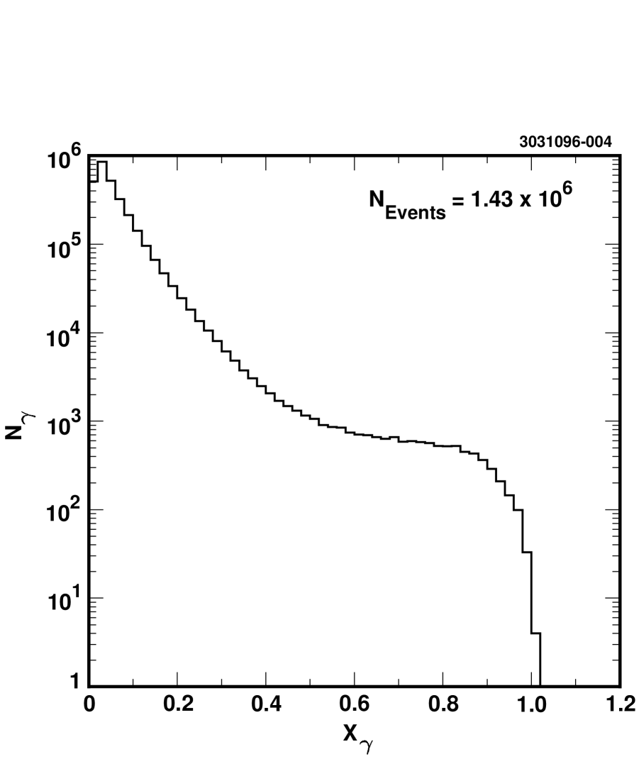
FIG. 1.: The inclusive distribution of candidate photons as a function of scaled momentum $X_{\gamma}\equiv p_{\gamma}/E_{beam}$, from data taken at the $\Upsilon{\rm(1S)}$ center-of-mass energy. Note the log scale of the y-axis.

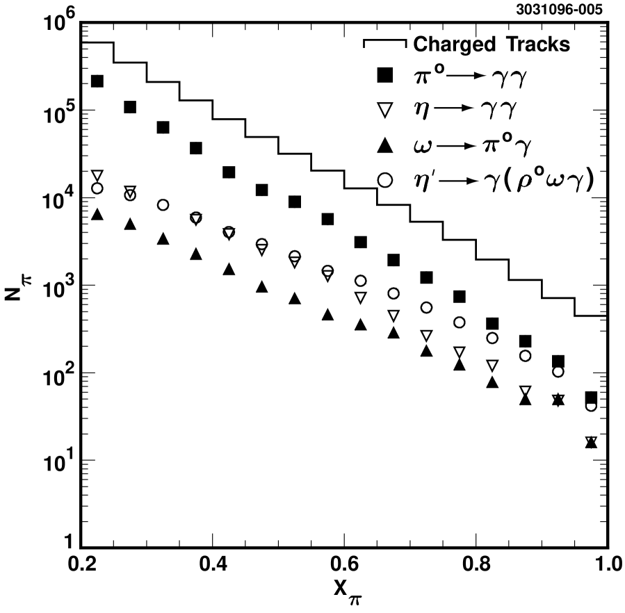
FIG. 2.: Efficiency corrected $\pi^{0}$ momentum spectrum, Monte Carlo generated $\eta$, $\eta^{\prime}$, and $\omega$ spectra, and observed charged tracks’ momentum spectrum as a function of scaled particle momentum, $X_{\pi}=p_{\pi}/E_{\rm beam}$. In this notation, ‘$\pi$’ refers to any of the neutral spectra or charged tracks.

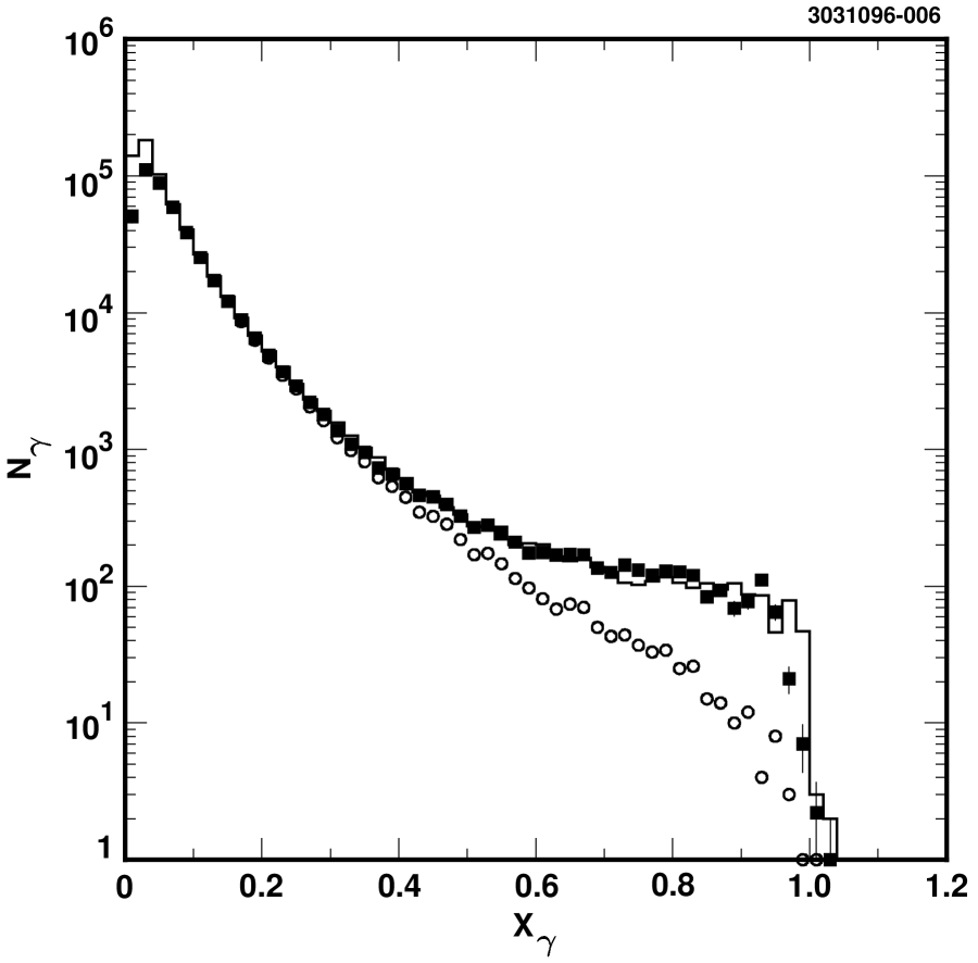
FIG. 3.: A comparison of the inclusive photon spectrum from continuum data taken below the $\Upsilon(4{\rm S})$ resonance (histogram) with the simulated background spectrum from $\pi^{0}$’s, $\eta$’s, $\eta^{\prime}$’s, and $\omega$’s produced by non-resonant processes at this energy. To illustrate the magnitude of the initial state radiative (ISR) correction, the simulated spectrum both with (dark squares) and without (open circles) the (Monte Carlo determined) radiative contribution are overlaid.

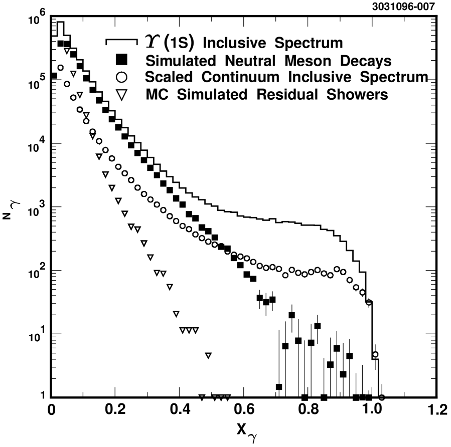
FIG. 4.: The inclusive $X_{\gamma}$ spectrum (histogram) for data taken at the $\Upsilon({\rm 1S})$ resonance, along with background contributions due to non-resonant processes (open circles), resonant hadronic decays (dark squares), and other residual sources (inverted triangles).

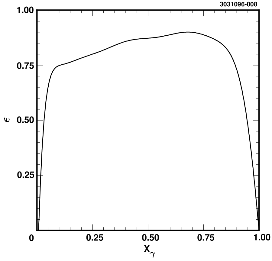
FIG. 5.: The direct photon detection efficiency as a function of scaled photon momentum $X_{\gamma}$, determined by averaging the two Monte Carlo simulation models (see text).

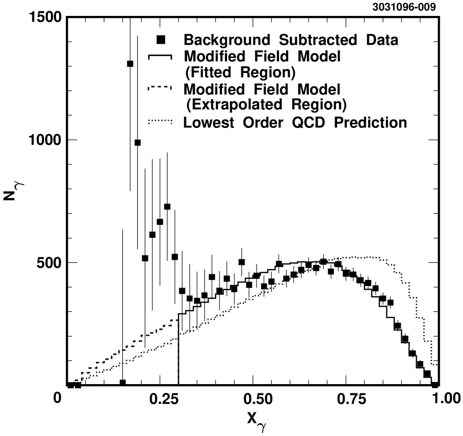
FIG. 6.: The background subtracted (i.e., direct) photon spectrum (dark squares). The data points in the region $0.3<X_{\gamma}<0.98$ are fit to Field’s model (histogram). The only free parameter in the fit was the overall normalization. The fit to Field’s model, extrapolated into the low momentum region, is also shown (dashed line) as well as the lowest order QCD prediction (dotted line) over the full kinematic regime, which has been normalized to the same area as the Field model. The errors shown are purely statistical. Data points in the region $X_{\gamma}<0.3$ appear systematically shifted above the Field line, however, a one sigma shift in the magnitude of the simulated background line in Figure 4 would drastically alter the distribution at the low $X_{\gamma}$ end. Systematic errors, had they been included on these points, would be well off scale.

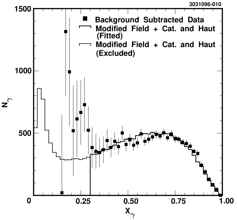
FIG. 7.: The background subtracted photon spectrum (dark squares) fit to the Field distribution with the added fragmentation component predicted by Catani and Hautmann. Again, the errors shown on the data points are purely statistical.

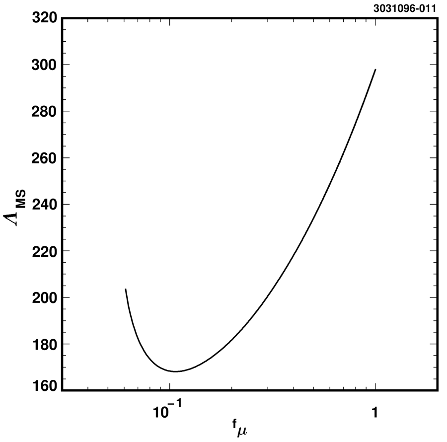
FIG. 8.: $\Lambda_{\overline{MS}}$ as a function of scale parameter $f_{\mu}$, as governed by the functional dependence of $R_{\gamma}$ on $\Lambda_{\overline{MS}}$ and $f_{\mu}$.

REFERENCES

- [1] CLEO Collab., Y. Kubota , “The CLEO-II detector”, Nucl. Instr. Meth. A320, 66 (1992).
- [2] S.J. Brodsky, T.A.DeGrand, R.R. Horgan and D.G. Coyne, Phys. Lett. B73 (1978) 203; K. Koller, and T. Walsh, Nucl. Phys. B140, (1978) 449.
- [3] D.M. Photiadis, Phys. Lett. B164 (1985) 160.
- [4] S. Catani and F. Hautmann, Nucl. Phys. B, Proc. Suppl. 39BC, 359 (1995).
- [5] R.D. Field, Phys. Lett. B133 (1983) 248.
- [6] David N. Brown, Ph.D. Dissertation, Purdue University (1992), unpublished.
- [7] S. J. Sjostrand, LUND 7.3, CERN-TH-6488-92 (1992).
- [8] R. Brun et. al., GEANT v. 3.14, CERN Report No. CERN CC/EE/84-1 (1987).
- [9] K. Koller, and T. Walsh, ref [2].
- [10] Review of Particle Properties, Phys. Rev. D54, (1996).
- [11] H. Albrecht et al., ARGUS Collab., Z. Phys. C54 (1992) 13.
- [12] S.E. Csorna et al., CLEO Collab., Phys. Rev. Lett. 56 (1986) 1222.
- [13] H. Albrecht et al., ARGUS Collab., Phys. Lett. B199 (1987) 291.
- [14] A. Bizzeti et al., CRYSTAL BALL Collab., Phys. Lett. B267 (1991) 286.
- [15] S. Sanghera, Int’l Journal of Mod. Phys. A9, (1994) 5743, and S. Sanghera, Ph. D. Thesis, Carleton U. (1991), unpublished, and S. Sanghera, private communication.
- [16] P. B. Mackenzie and G. Peter Lepage, in Perturbative Quantum Chromodynamics, Conf. Proceed., Tallahassee, 1981, AIP, New York, 1981.
- [17] W. A. Bardeen et al., Phys. Rev. D18 (1978) 3998.
- [18] S. J. Brodsky, G. P. Lepage and P. B. Mackenzie, Phys. Rev. D28 (1983) 228.
- [19] P. B. Mackenzie and G. Peter Lepage, Phys. Rev. Lett. 47 (1981) 1244.
- [20] G. Grunberg, Phys. Lett. B95 (1980) 70.
- [21] P.M. Stevenson, Phys. Rev. D23 (1981) 2916.
- [22] W. J. Marciano, Phys. Rev. D29 (1984) 580.
- [23] S. Bethke, Proc. International Conf. on High Energy Phys., Dallas TX, August 1992.
- [24] A. C. Benvenuti, BCDMS Collab., Phys. Lett B223 (1989) 490.