A Study of $\bar{p}p\rightarrow$ Two Neutral Pseudoscalar Mesons at the $\chi_{c0}(1^{3}P_{0})$ Formation Energy

Abstract

Fermilab experiment E835 has studied reactions $\bar{p}p\rightarrow\pi^{0}\pi^{0},\,\pi^{0}\eta,\,\eta\eta,\,$ $\pi^{0}\eta^{\prime}$ and $\eta\eta^{\prime}$ in the energy region of the $\chi_{c0}(1^{3}P_{0})$ from $3340$ MeV to $3470$ MeV. Interference between resonant and continuum production is observed in the $\pi^{0}\pi^{0}$ and $\eta\eta$ channels, and the product of the input and output branching fractions is measured. Limits on resonant production are set for the $\pi^{0}\eta$ and $\pi^{0}\eta^{\prime}$ channels. An indication of interference is observed in the $\eta\eta^{\prime}$ channel. The technique for extracting resonance parameters in an environment dominated by continuum production is described.

I Introduction

E835 has measured the cross section of antiproton-proton annihilation into two pseudoscalar mesons ($\bar{p}p\rightarrow P_{1}P_{2}$) in the energy region of the $\chi_{c0}$. The final states studied are:

$$P_{1}P_{2}~{}\equiv~{}\pi^{0}\pi^{0}~{}\mathrm{(1)},~{}\pi^{0}\eta~{}\mathrm{(2)},~{}\eta\eta~{}\mathrm{(3)},~{}\pi^{0}\eta^{\prime}~{}\mathrm{(4)},~{}\mathrm{and}~{}\eta\eta^{\prime}~{}\mathrm{(5)}.$$

A total integrated luminosity of 33 pb^-1 has been collected at 17 energy points from 3340 MeV to 3470 MeV. The mesons were detected through their decay into two photons. The cross sections reported here have been corrected for the respective branching ratios PDG : $B(\pi^{0}\rightarrow\gamma\gamma)=(98.798\pm 0.032)\%$, $B(\eta\rightarrow\gamma\gamma)=(39.43\pm 0.26)\%$, and $B(\eta^{\prime}\rightarrow\gamma\gamma)=(2.12\pm 0.14)\%$.

The analysis of reaction (1) has been published in letter format 2pi0 . In the present work, processes (2)-(5) are reported for the first time and a more extensive discussion is given of process (1). More details on the analyses (1)-(3) can be found in a dissertation Paolo .

The expression for the angular distribution of $\bar{p}p\rightarrow P_{1}P_{2}$, in the vicinity of the $\chi_{c0}$ resonance, is given in Equations (6), (7) and (8). The subsequent isotropic decay of each meson into two photons need only to be considered for acceptance determination.

$$\frac{d\sigma}{dz}=\Big{|}-\frac{A_{R}}{x+i}+Ae^{i\delta_{A}}\Big{|}^{2}+\Big{|}Be^{i\delta_{B}}\Big{|}^{2},$$ (6)

$$A~{}e^{i\delta_{A}}\equiv\sum_{J=0,2,4,\,...}^{J_{max}}(2J+1)~{}C_{J}~{}e^{i\delta_{J}}~{}P_{J}(z),\mbox{~{}and}$$ (7)

$$B~{}e^{i\delta_{B}}\equiv\sum_{J=2,4,\,...}^{J_{max}}\frac{2J+1}{\sqrt{J(J+1)}}~{}C_{J}^{1}~{}e^{i\delta_{J}^{1}}~{}P_{J}^{1}(z).$$ (8)

The variable $z$ is defined as

$$z\equiv|\cos\theta^{*}|~{},$$ (9)

where $\theta^{*}$ is the production polar angle of the two mesons in the center of mass (cm), while $x$ is defined as

$$x\equiv\frac{E_{cm}-M_{\chi_{c0}}}{\Gamma_{\chi_{c0}}/2}.$$ (10)

The term $Ae^{i\delta_{A}}$ is generated from the $\bar{p}p$ state with helicity $\lambda_{i}\equiv\lambda_{p}-\lambda_{\bar{p}}=0$ (helicity-0), where $\lambda_{p}$ and $\lambda_{\bar{p}}$ are the proton and antiproton helicities, respectively. The helicity-0 coefficients and phases of the expansion are $C_{J}$ and $\delta_{J}$, respectively, while $P_{J}(z)$ are Legendre polynomials.

Figure 1: The first Legendre polynomials $P_{J}^{M=0}\equiv P_{J}$ (left) and associated functions $P_{J}^{M=1}$ (right).

The term $Be^{i\delta_{B}}$ is generated from the $\bar{p}p$ state with helicity $|\lambda_{i}|=1$ (helicity-1). The helicity-1 coefficients and phases are $C_{J}^{1}$ and $\delta_{J}^{1}$, respectively, while $P_{J}^{1}(z)$ are Legendre associate functions $P_{J}^{M}$ with $M=1$. The $\chi_{c0}$ ($1^{3}P_{0}$) resonance, parameterized by a Breit-Wigner amplitude $-A_{R}/(x+i)$, has been extracted from the $J=0$ term. Both nonresonant terms, $Ae^{i\delta_{A}}$ and $Be^{i\delta_{B}}$, have a slowly varying (on the scale of the $\chi_{c0}$ width, $\approx 10$ MeV) dependence on $x$ and an angular dependence on $z$ described by the Legendre polynomials. The amplitudes $-A_{R}/(x+i)$ and $Ae^{i\delta_{A}}$, from the same helicity-0 initial state add coherently and interfere with each other. The amplitude $Be^{i\delta_{B}}$ is added incoherently because it is generated from the helicity-1 initial state and does not interfere with the helicity-0 terms.

Equation (6) can also be written as

$$\frac{d\sigma}{dz}=\frac{A_{R}^{2}}{x^{2}+1}+A^{2}+\underbrace{2A_{R}A\,\frac{\sin{\delta_{A}}-x\cos{\delta_{A}}}{{x^{2}+1}}}_{\mathrm{interference-term}}+B^{2}.$$ (11)

Given the moderate energy dependence of $Ae^{i\delta_{A}}$ and $Be^{i\delta_{B}}$, Equation (11) shows that at a fixed value of $z$, as $E_{cm}$ varies across the resonance, even a small resonant contribution can generate a significant interference signal superimposed on the continuum. As an example, for a resonant amplitude $A_{R}$ that is one tenth of the helicity-0 continuum amplitude $A$, the peak contribution to the cross section from the Breit-Wigner term $A_{R}^{2}/(x^{2}+1)$ is only 1% of $A^{2}$, while the factor $2A_{R}A$ of the interference term of Equation (11) is 20% of $A^{2}$. The factor $(\sin{\delta_{A}}-x\cos{\delta_{A}})/(x^{2}+1)$ determines the shape of the interference pattern. A small resonance and a large continuum is a typical experimental condition found when studying charmonium in the process $\bar{p}p\rightarrow\mathrm{hadrons}$.

The term $B^{2}$ provides an additional contribution to the cross section, and if $B^{2}$ is too large compared to the interference term, it may mask the presence of the resonance. It is quite helpful that the associated Legendre functions with $M=1$, which are the constituents of the amplitude $Be^{i\delta_{B}}$, share a common multiplicative factor $z$ which causes them to vanish at $z=0$ (see Figure 1). Since the polynomials $P_{J}^{1}$ are either squared or multiplied by each other, $B^{2}$ is suppressed with respect to $A^{2}$ by $z^{2}$ at small $z$. To measure the value of the resonant amplitude $A_{R}$, it is critical to know the size of both the helicity-0 continuum, with which the resonance is coherent, and the helicity-1 continuum, which is incoherent with the resonance. The region at small $z$ (i.e. $\cos\theta^{*}\approx 0)$ is therefore the natural place to concentrate for the determination of $A_{R}$.

Table 1: How the orbital angular momentum $L$ and the spin $S$ of the $\bar{p}p$ in the initial state combine to make different $J^{PC}$ values and the corresponding charmonium resonances. A $\checkmark$ indicates whether a pseudoscalar-pseudoscalar ($P_{1}P_{2}$) state is accessible. Spectroscopic notation is given for $\bar{p}p$ (${}^{2S+1}L_{J}$) and $c\bar{c}$ ($n^{2S+1}L_{J}$).

$\bar{p}p$			$\bar{c}c$		$P_{1}P_{2}$
$L~{}~{}S$	${}^{2S+1}L_{J}$	$J^{PC}$	resonance	$n^{2S+1}L_{J}$
$0~{}~{}0$	${}^{1}S_{0}$	$0^{-+}$	$\eta_{c}~{}(\eta^{\prime}_{c})$	$1^{1}S_{0}~{}(2^{1}S_{0})$
$0~{}~{}1$	${}^{3}S_{1}$	$1^{--}$	$J/\psi~{}(\psi^{\prime})$	$1^{3}S_{1}~{}(2^{3}S_{1})$
$1~{}~{}0$	${}^{1}P_{1}$	$1^{+-}$	$h_{c}$	$1^{1}P_{1}$
$1~{}~{}1$	${}^{3}P_{0}$	$0^{++}$	$\chi_{c0}$	$1^{3}P_{0}$	$\checkmark$
$1~{}~{}1$	${}^{3}P_{1}$	$1^{++}$	$\chi_{c1}$	$1^{3}P_{1}$
$1~{}~{}1$	${}^{3}P_{2}$	$2^{++}$	$\chi_{c2}$	$1^{3}P_{2}$	$\checkmark$
$2~{}~{}0$	${}^{1}D_{2}$	$2^{-+}$
$2~{}~{}1$	${}^{3}D_{1}$	$1^{--}$	$\psi^{\prime\prime}$	$1^{3}D_{1}$
$2~{}~{}1$	${}^{3}D_{2}$	$2^{--}$
$2~{}~{}1$	${}^{3}D_{3}$	$3^{--}$
$3~{}~{}0$	${}^{1}F_{3}$	$3^{+-}$
$3~{}~{}1$	${}^{3}F_{2}$	$2^{++}$			$\checkmark$
$3~{}~{}1$	${}^{3}F_{3}$	$3^{++}$
$3~{}~{}1$	${}^{3}F_{4}$	$4^{++}$			$\checkmark$
$4~{}~{}0$	${}^{1}G_{4}$	$4^{-+}$
$4~{}~{}1$	${}^{3}G_{3}$	$3^{--}$
$4~{}~{}1$	${}^{3}G_{4}$	$4^{--}$
$4~{}~{}1$	${}^{3}G_{5}$	$5^{--}$

Table 1 shows how the orbital angular momentum ($L_{\bar{p}p}$) and spin ($S_{\bar{p}p}$) combine to form different values of the total angular momentum, parity and charge conjugation ($J^{PC}$). For each $J^{PC}$, it shows which charmonium resonance is formed, and whether the $J^{PC}=\mathrm{even}^{++}$ pseudoscalar-pseudoscalar final states can be accessed. The spectroscopic notation (${}^{2S+1}L_{J}$) is given for $\bar{p}p$ and $c\bar{c}$ states. Both states are fermion-antifermion, thus are described in the same way as far as $L$, $S$ and $J^{PC}$ are concerned, while a radial quantum number ($n$) applies only to the bound $c\bar{c}$ system. The $\chi_{c0}$ ($J^{PC}=0^{++}$) can be produced only from the spin-triplet $L_{\bar{p}p}=1$. Table 1 is sorted by increasing $L_{\bar{p}p}$, which correlates with the $\bar{p}p$ impact parameter ($b$). Even for nonresonant reconfiguration of the $\bar{p}p$ system into two pseudoscalar mesons, small impact parameter is favored at small $z$ since the valence quarks must either annihilate or suffer large momentum transfers. Excellent fits to the angular distributions of the two pseudoscalar mesons are obtained with a limited number of partial waves.

II Data Selection

A comprehensive description of the E835 apparatus and experimental technique is provided in bigpaper . The data selection and the determination of the acceptance and efficiency for the processes (1)-(3) are extensively discussed in Paolo ; only a summary is given here. Processes (4) and (5) are discussed in Section X.

The stochastically-cooled $\bar{p}$ beam circulating in the antiproton accumulator intercepts a hydrogen gas-jet target. The energy of the beam can be tuned to the energy of interest. Before the year 2000 run, the accumulator transition energy was raised to $E_{cm}$ of 3600 MeV. A technique was developed to modify the accumulator lattice and lower the transition energy as the beam was decelerated McGinnis:gt , thus allowing adequate margin between the operating energy and the transition energy. The $E_{cm}$ spectrum is approximately gaussian and is determined from measurements of the $\bar{p}$-beam revolution frequency and orbit length. The precision of the measurement of the mean value of the $E_{cm}$ spectrum is about 100 keV. The r.m.s. spread of the $E_{cm}$ spectrum is a few hundred keV, much smaller than the width of the $\chi_{c0}$ resonance.

The important detectors for this analysis are the central calorimeter (CCAL) which is used to measure the photon energy deposits, the system of scintillation counters which vetoes events with charged particles and the luminosity monitor. The energy resolution of CCAL is $\sigma_{E}/E\simeq 6\%/\sqrt{E(\mathrm{GeV})}+1.4\%$, while the polar and azimuthal angular resolutions are $\sigma_{\theta}\simeq 6$ mrad and $\sigma_{\phi}\simeq 11$ mrad, respectively.

Online, two-body candidate events were selected by means of two independent triggers based on CCAL: the two-body trigger and the total-energy trigger. The two-body trigger accepted events with two large energy deposits in CCAL satisfying two-body kinematics; the total-energy trigger accepted events where at least 80% of the center-of-mass energy was deposited in CCAL. For $\pi^{0}\pi^{0}$ events, the efficiency of the two-body trigger is $99.9\%$ - the small opening angles of the decay $\pi^{0}\rightarrow\gamma\gamma$ keeps the $\pi^{0}\pi^{0}\rightarrow 2\gamma+2\gamma$ events within the two-body trigger requirements - while the efficiency of the total-energy trigger is $\sim 98.2\%$. The two-body trigger is somewhat less efficient for $\eta\rightarrow\gamma\gamma$ decays and only the total-energy trigger was used for selecting $\pi^{0}\eta$ and $\eta\eta$ events, with an average efficiency of $\sim 98.5\%$ for both channels. Both triggers were subjected to the charged-particle veto.

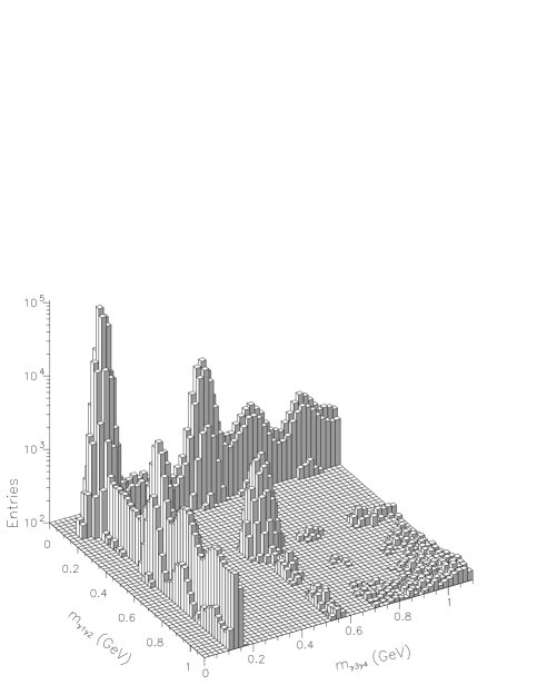
Figure 2: LEGO plot of the two 2-photon invariant masses $m_{\gamma_{1}\gamma_{2}}$ and $m_{\gamma_{3}\gamma_{4}}$. Note the logarithmic scale of the vertical axis.

Offline, events with four CCAL energy deposits greater than 100 MeV are retained if they passed a 5% probability cut on a 4-constraint (4C) fit to $\bar{p}p\rightarrow 4\gamma$. There are three ways to combine the four photons into two pairs; the event topology was chosen as the combination with the highest confidence level of a 6C fit to $\bar{p}p\rightarrow P_{1}P_{2}\rightarrow 4\gamma$. However, given the limited opening angles of the decay $\pi^{0}(\mathrm{or}~{}\eta)\rightarrow\gamma\gamma$ at these energies and the large angle between the two mesons, it is virtually impossible that more than one combination satisfy the 6C fits for more than one of the processes (1)-(3). Figure 2 is a LEGO plot of the two 2-photon invariant masses prior to any fitting. Evident are high peaks of $\pi^{0}\pi^{0}$, $\pi^{0}\eta$ and $\eta\eta$ events, as well as those of $\pi^{0}\omega$ (where a photon in the $\omega\rightarrow\pi^{0}\gamma\rightarrow\gamma\gamma\gamma$ decay chain is not observed), $\pi^{0}\eta^{\prime}$ and $\eta\eta^{\prime}$. Marked “berms” are produced by $\pi^{0}X$ events, where $X$ can be one or more particles that partially escaped detection. Softer $\eta X$ berms are also noticeable. Prior to a 4C fit, the mass resolution for a $\pi^{0}$, an $\eta$, and an $\eta^{\prime}$ is $\sigma$$\simeq$$15$ MeV, $25$ MeV and $35$ MeV, respectively, with a small dependence on $z$.

Table 2: The kinematic cuts applied to each channel. The asymmetry of the cut on the invariant mass reconstructed of the candidate $\pi^{0}$ compensates for a slight overestimate of the invariant mass reconstructed for $\pi^{0}$’s when the energy deposits from the daughter photons overlap in the CCAL (see details in bigpaper ).

Channel	$|\Delta\theta|$	$|\Delta\phi|$	$m_{\gamma_{1}\gamma_{2}}$ cut	$m_{\gamma_{3}\gamma_{4}}$ cut
$\pi^{0}\,\pi^{0}$	12 mrad	30 mrad	$100$ MeV - $185$ MeV	$100$ MeV - $185$ MeV
$\pi^{0}\,\eta~{}$	14 mrad	38 mrad	$100$ MeV - $185$ MeV	$M_{\eta}\pm 70$ MeV
$\eta\,\eta~{}~{}$	15 mrad	45 mrad	$M_{\eta}\pm 70$ MeV	$M_{\eta}\pm 70$ MeV
$\pi^{0}\,\eta^{\prime}$	18 mrad	50 mrad	$100$ MeV - $185$ MeV	$M_{\eta^{\prime}}\pm 40$ MeV
$\eta\,\eta^{\prime}~{}$	18 mrad	50 mrad	$M_{\eta}\pm 45$ MeV	$M_{\eta^{\prime}}\pm 40$ MeV

A set of kinematic cuts is applied for each process with the values shown in Table 2. These include cuts on the invariant masses of each pair of photons and on the colinearity and coplanarity of the candidate mesons. The colinearity, $\Delta\theta$, of the two mesons A and B, is given by $\theta_{\mathrm{meas}}^{\mathrm{A}}-\theta_{\mathrm{calc}}^{\mathrm{A}}$, where $\theta_{\mathrm{meas}}^{\mathrm{A}}$ is the measured polar angle of meson A while $\theta_{\mathrm{calc}}^{\mathrm{A}}$ is the value of the same quantity calculated assuming two-body kinematics using the measured polar angle of meson B. In the case where the two mesons are the same, A is chosen to be the one in the forward direction. In the case where they are different, A is chosen to be the lighter of the two mesons. The coplanarity, $\Delta\phi$, is defined as $180^{\circ}-|\phi_{\mathrm{meas}}^{\mathrm{A}}-\phi_{\mathrm{meas}}^{\mathrm{B}}|$, where $\phi_{\mathrm{meas}}^{\mathrm{A}}$ and $\phi_{\mathrm{meas}}^{\mathrm{B}}$ are the measured azimuthal angles of the mesons.

Figure 3: The product of detector acceptance and selection efficiency, $a$$\times$$\epsilon$, as a function of $z$ for $\pi^{0}\pi^{0}$, $\pi^{0}\eta$ and $\eta\eta$ events. In the $\pi^{0}\eta$ case, where the two mesons are distinguishable, $z$ is defined as $\cos\theta^{*}_{\pi^{0}}$.

The selection efficiency ($\epsilon$) and detector acceptance ($a$) are determined by Monte Carlo (MC) simulation. MC events are generated with a uniform angular distribution and a matrix is built to record both the generated and reconstructed values of $z$. The angular distribution of the data is determined by using the inverse of this matrix to correct for effects due to the angular resolution of the detector. The product of the acceptance and efficiency ($a$$\times$$\epsilon$) as a function of the generated value of $z$ for $\pi^{0}\pi^{0}$, $\pi^{0}\eta$ and $\eta\eta$ is shown in Figure 3.

A significant source of inefficiency is event pileup. It is particularly important to correct for this effect since it is rate dependent and the instantaneous luminosity varied from one energy point to another. To determine the pileup effects, MC events were overlaid with the contents of random-gate events recorded throughout the data-taking, thus reproducing the conditions of each energy point. The event reconstruction was then performed on these hybrid events to determine the reconstruction efficiency. The rate-dependent losses vary from 14% to 23% with an average of 20%; these losses do not differ significantly among the analyzed reactions. As a function of $z$, the pileup correction is determined and applied.

III Signal and Background Subtraction for $\pi^{0}\pi^{0}$, $\pi^{0}\eta$ and $\eta\eta$ samples.

Figure 4 shows the region of the $\pi^{0}\pi^{0}$ peak before applying the mass cuts. A log-likelihood fit is performed to this data. The function used is the sum of a two gaussians, having the same mean, to describe the $\pi^{0}\pi^{0}$ peak, and two gaussian berms and a tilted plane to describe the background (from events such as $\pi^{0}\omega\rightarrow\pi^{0}\pi^{0}\gamma$ and $\pi^{0}\pi^{0}\pi^{0}$ where, respectively, one and two photons are not observed). The background component of the fitted function is shown as a gray surface. The background is estimated and subtracted as a function of $z$ as indicated in Figure 7 and amounts to ($2-2.5$)% for $z<0.3$ and ($1.5-2$)% for $0.3<z<0.6$.

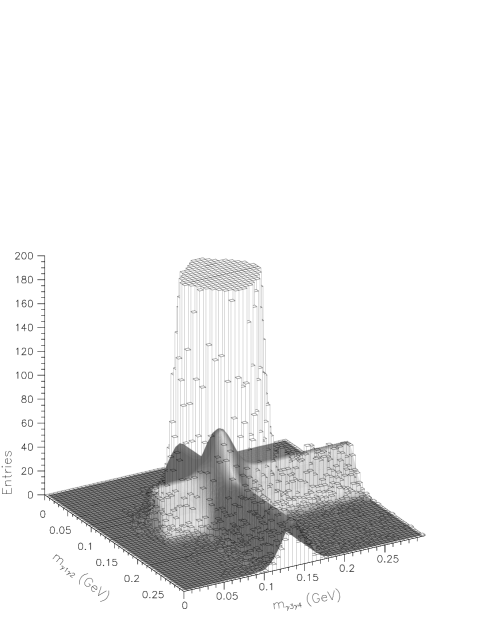
Figure 4: The region of the $\pi^{0}\pi^{0}$ peak (truncated at about 2% of its height) with a fit to the background shown as a gray surface.

A similar procedure is used in Figure 5 for determining the background at the $\pi^{0}\eta$ peak, which amounts to a total of $11\%$ over the range $-0.6<z<0.6$ and is distributed as shown in Figure 7.

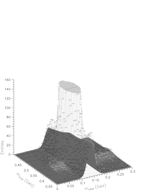
Figure 5: The region of the $\pi^{0}\eta$ peak (truncated at about 20% of its height) with a fit to the background shown as a gray surface.

Figure 6 shows the $\eta\eta$ peak and its fitted background, amounting to a total of $8\%$ over the range $0<z<0.6$ with the angular distribution shown in Figure 7.

Figure 6: The region of the $\eta\eta$ peak (truncated at about 12% of its height) with a fit to the background shown as a gray surface.

Figure 7: The number of candidate events (Tot) as a function of $z$ at the $\chi_{c0}$ mass, the estimated background events (Bkgd), and a polynomial fit (solid curve) to the number of background events. Corrections for detector acceptance and efficiency have not yet been applied. For the $\eta\eta$ channel, the background distribution was independent of energy and the data from all 17 energy points have been merged to reduce bin-to-bin fluctuations.

IV The $\pi^{0}\pi^{0}$ Cross Section

A paper on the $\pi^{0}\pi^{0}$ reaction has been published 2pi0 . The measured $\bar{p}p\rightarrow\pi^{0}\pi^{0}$ differential cross section is shown in Figure 8 for 3 of the 17 energy points of the data sample and over an angular range limited to $0<z<0.6$ by the detector acceptance. The cross section integrated to various values of $z_{max}$ is shown in Figure 9 for all energy points.

Figure 8: The $\bar{p}p\rightarrow\pi^{0}\pi^{0}$ differential cross section versus $z\equiv|\cos\theta^{*}|$ at different $E_{cm}$. A fit using Equations (6)-(8), with values from Table 3, is shown.

Figure 9: The measured $\bar{p}p\rightarrow\pi^{0}\pi^{0}$ cross section integrated over $0<z<z_{max}$ plotted versus $E_{cm}$. A fit using Equations (6)-(8) is shown.

Figures 8 and 9 also show a binned maximum-likelihood fit to the cross section. The fit is performed simultaneously on all 17 energy points and over $0<z<0.6$. Within this range, the number of background-subtracted $\pi^{0}\pi^{0}$ events is 431,625. The parameterization of Equations (6)-(8) is used setting $J_{max}=4$; the number of partial waves to include and their energy dependence were determined by searching for significant improvements of the $\chi^{2}$. The mass and width of the $\chi_{c0}$ are constrained to the values (see Table 4) determined by studying the process $\bar{p}p\rightarrow J/\psi\,\gamma;J/\psi\rightarrow e^{+}e^{-}$ psigamma . A magnified version of the plot of $d\sigma/dz$ at $E_{cm}=3415$ MeV, as well as a detailed description of the fit and its different components, is provided in 2pi0 . The fit results are given in Table 3.

Table 3: Fit results for coefficients and phases of the partial-wave expansion of Equations (6)-(8) for the $\pi^{0}\pi^{0}$, $\pi^{0}\eta$ and $\eta\eta$ channels. A linear energy dependence is included when found necessary. The errors are statistical.

	$C_{J}~{}[~{}\mathrm{nb}^{1/2}~{}]~{}\&~{}C_{J}^{1}~{}[~{}\mathrm{nb}^{1/2}~{}]$	$\delta_{J}~{}[~{}\mathrm{degree}~{}]~{}\&~{}\delta_{J}^{1}~{}[~{}\mathrm{degree}~{}]$
	$C_{0}=(12.8\pm 0.7)-(0.19\pm 0.02)x$	$\delta_{0}=-36.1\pm 1.8$
	$C_{2}=(8.3\pm 0.4)-(0.055\pm 0.010)x$	$\delta_{2}=-43.0\pm 1.0$
$\pi^{0}\pi^{0}$	$C_{4}=(2.5\pm 0.2)+(0.022\pm 0.003)x$	$\delta_{4}=-15.1\pm 1.2$
	$C_{2}^{1}=(5.19\pm 0.13)-(0.063\pm 0.005)x$	$-$
	$C_{4}^{1}=(1.52\pm 0.09)-(0.021\pm 0.003)x$	$\delta_{4}^{1}-\delta_{2}^{1}=-0.7\pm 0.2$
	$C_{0}=(19.7\pm 0.3)-(0.076\pm 0.003)x$	$-$
	$C_{2}=(12.2\pm 0.2)$	$\delta_{2}-\delta_{0}=4.5\pm 0.8$
$\pi^{0}\eta$	$C_{4}=(3.21\pm 0.09)$	$\delta_{4}-\delta_{0}=9\pm 2$
	$C_{2}^{1}=(2.8\pm 0.2)-(0.129\pm 0.008)x$	$-$
	$C_{4}^{1}=(2.54\pm 0.09)-(0.087\pm 0.004)x$	$\delta_{4}^{1}-\delta_{2}^{1}=0$
	$C_{0}=(7.27\pm 0.11)-(0.269\pm 0.012)x$	$\delta_{0}=138.2\pm 2.9$
	$C_{2}=(2.07\pm 0.06)-(0.116\pm 0.006)x$	$\delta_{2}=138.2\pm 2.9$
$\eta\eta$	$C_{4}=0$	$\delta_{4}=138.2\pm 2.9$
	$C_{2}^{1}=(4.56\pm 0.07)x$	$-$
	$C_{4}^{1}=(2.65\pm 0.05)x$	$\delta_{4}^{1}-\delta_{2}^{1}=0$

The fit presented in this section demonstrates the general structure of the $\bar{p}p\rightarrow\pi^{0}\pi^{0}$ angular distribution and estimates the number and amount of the contributing partial waves. However, this fit is not very sensitive to the value of the resonant amplitude $A_{R}$. The reason is that the size of the (interference-enhanced) resonant signal is significant only at small values of $z$, while the fit is dominated by the high statistics of the nonresonant forward peak. The next section describes how the extraction of $A_{R}$ is carried out.

V Extraction of $B(\chi_{c0}\rightarrow\bar{p}p)\times B(\chi_{c0}\rightarrow\pi^{0}\pi^{0})$

As discussed in Section I (see in particular the discussion of Equation 11), the natural region to exploit in order to obtain a model-insensitive measurement of the resonance amplitude $A_{R}$ is the region at small values of $z$.

To find the value of $z$ at which the noninterfering continuum starts to play a significant role, we perform independent fits in each bin $\Delta z$ at small $z$. Each fit uses the parameterization of Equation (6) with $Be^{i\delta_{B}}$ set equal to zero. The parameterization used for the helicity-0 component of the continuum is

$$A^{2}\equiv a_{0}+a_{1}x+a_{2}x^{2}\,,$$ (12)

to reproduce the moderate energy dependence of the cross section, see Figure 9.

Since the growth with $z$ of the helicity-1 component is not accounted for in these fits, the estimate of $A_{R}$, which in reality is a constant, will show an artificial decrease at values of z where the helicity-1 component can no longer be neglected. The value of $A_{R}$ can then be derived by using all the data up to some maximum value of $z$ identified by the fits to the individual bins. The fit results for $A_{R}$ from individual bins of $\Delta z$ up to $z=0.3$ are shown in Figure 10-top and the values of $A_{R}$ derived by using the data within $0<z<z_{max}$ are shown in Figure 10-bottom.

The observed drop in $A_{R}$ of Figure 10-top at $z\gtrsim 0.15$ shows that the helicity-1 component is no longer negligible at this value of $z$. We therefore restrict our region to

$$z\leq z_{max}\equiv 0.125$$ (13)

The restricted $z$ range increases the statistical uncertainty on $A_{R}$, but ensures there is little effect on $A_{R}$ from systematic uncertainties in our knowledge of $B$. The fit is described in detail in 2pi0 and is reproduced in Figure 11.

Figure 10: Fits for the resonant amplitude of $\bar{p}p\rightarrow\chi_{c0}\rightarrow\pi^{0}\pi^{0}$. Top: the fits are to the data of each bin in $\Delta z=0.025$. $B$ is set to zero (see text). Bottom: each fit is performed over a range $0<z<z_{max}$ for increasing $z_{max}$ and $|B~{}e^{i\delta_{B}}|^{2}$ is inserted from the fit of Figure 8. (The inner error bars are statistical while the outer ones indicate the uncertainty on $C_{2}^{1}$, $C_{4}^{1}$ and $\delta_{4}^{1}$-$\delta_{2}^{1}$ in Table 3).

Figure 11: The $\bar{p}p\rightarrow\pi^{0}\pi^{0}$ cross section integrated over $0<z<0.125$ plotted versus $E_{cm}$. The fit of Equation 6 is shown along with its components. The contribution of $|B~{}e^{i\delta_{B}}|^{2}$ is constrained to the estimate obtained from the partial-wave expansion fit of Figure 8, and its integration corresponds to the separation between the curves $\int\,(A^{2}+B^{2})\,dz$ and $\int\,A^{2}\,dz$. The “pure” Breit-Wigner curve, $\int[A_{R}^{2}/(x^{2}+1)]\,dz$, is shown multiplied by a factor 20.

The value obtained for the resonant amplitude $A_{R}$ is given by:

$$A_{R}^{2}=\pi\lambdabar^{2}\times B(\chi_{c0}\rightarrow\bar{p}p)\times B(\chi_{c0}\rightarrow\pi^{0}\pi^{0})~{},$$ (14)

where $\lambdabar$ is the center-of-mass de Broglie wavelength, which gives:

$$B(\chi_{c0}\rightarrow\bar{p}p)\times B(\chi_{c0}\rightarrow\pi^{0}\pi^{0})=(5.09\pm 0.81\pm 0.25)\times 10^{-7}~{}.$$ (15)

The uncertainties are statistical and systematic, respectively. The dominant systematic errors arise from the luminosity determination (2.5%) and the knowledge of $M_{\chi_{c0}}$ from psigamma (2.5%). The systematic error due to the uncertainty in the helicity-1 continuum $|B~{}e^{i\delta_{B}}|^{2}$ is $1.2\%$.

The phase between the helicity-0 nonresonant amplitude $A$ and the resonant amplitude $A_{R}$ is $\delta_{A}=(39\pm 5\pm 6)~{}\mathrm{degrees}$. In the region $0<z<0.125$ of the fit, no dependence of $\delta_{A}$ on $z$ and $x$ is found. The values of $\delta_{0}$, $\delta_{2}$, and $\delta_{4}$ are given in Table 3.

VI The $\eta\eta$ Cross Section

The measured $\bar{p}p\rightarrow\eta\eta$ differential cross section is shown in Figure 12. Figure 13 shows the integrated cross section versus $E_{cm}$. As in the $\pi^{0}\pi^{0}$ case, the cross section is dominated by the nonresonant continuum $\bar{p}p\rightarrow\eta\eta$, which has a smooth dependence on the energy. The $\eta\eta$ channel also shows a resonance signal near the mass of the $\chi_{c0}$. The interference pattern is different from the one observed in the $\pi^{0}\pi^{0}$ channel. There is destructive interference on the low-energy side of the resonance and constructive on the high-energy side, with the resonance peak shifted to above the $\chi_{c0}$ mass.

Figure 12: The $\bar{p}p\rightarrow\eta\eta$ differential cross section versus $z\equiv|\cos\theta^{*}|$ at different $E_{cm}$. To reduce statistical fluctuations, the 17 energies are displayed merged as $3339.5$ MeV $<E_{cm}<3400.1$ MeV (left), $3406.1$ MeV $<E_{cm}<3430.1~{}$MeV (center) and $E_{cm}=3469.9$ MeV (right). A fit using Equations (6)-(8) is shown along with its components (see Table 3 for values of fit parameters).

Figure 13: The measured $\bar{p}p\rightarrow\eta\eta$ cross section integrated over $0<z<z_{max}$ plotted versus $E_{cm}$. A fit using Equations (6)-(8) is shown.

As in the $\pi^{0}\pi^{0}$ analysis, a binned maximum-likelihood fit to the $\bar{p}p\rightarrow\eta\eta$ differential cross section is performed simultaneously on all 17 energy points and over an angular range limited to $0<z<0.6$ by the detector acceptance. Within this range, there are 19,675 background-subtracted $\eta\eta$ events. The parameterization used is given in Equation 6, with the partial-wave expansion of Equations 7 and 8. The mass and width of the $\chi_{c0}$ are constrained to the values determined by means of the $J/\psi\,\gamma$ channel psigamma .

The result of the fit is shown in Figures 12 and 13. As in the $\pi^{0}\pi^{0}$ case, the contribution of the “pure” resonance, $A_{R}^{2}/(x^{2}+1)$, is negligible. The $B^{2}$ (helicity-1) term dominates at larger $z$, but its growth begins at a larger value of $z$ than in the $\pi^{0}\pi^{0}$ case. The interfering helicity-0 continuum, of magnitude $A^{2}$, dominates for a large part of the angular range ($0<z\lesssim 0.5$) and provides the amplification for the interference-enhanced resonance signal seen in the separation between $d\sigma/dz$ and $A^{2}+B^{2}$. Since the number of events available in the $\eta\eta$ channel is limited (about 20 times fewer than in the $\pi^{0}\pi^{0}$ channel), the angular distribution within the available range in $z$ is not as well resolved as in the $\pi^{0}\pi^{0}$ and $\pi^{0}\eta$ channels. Compared to the $\pi^{0}\pi^{0}$ and $\pi^{0}\eta$, the $\eta\eta$ channel requires a smaller number of parameters. In the best fit (see Table 3) $C_{0}$ and $C_{2}$ have a linear energy dependence; $C_{4}$ vanishes and is subsequently constrained to zero; and $C_{21}$ and $C_{41}$ do not require an energy dependence. The phases $\delta_{0}$, $\delta_{2}$ and $\delta_{4}$ are equal to each other, different from zero (that is the phase of the resonant amplitude is different from the phases of the nonresonant amplitudes) and constant in energy. The phases of the helicity-1 continuum (only the difference between $\delta_{4}^{1}$ and $\delta_{2}^{1}$ is measurable) also are not significantly different from each other and do not exhibit an energy dependence. Note that even in the $\pi^{0}\pi^{0}$ and $\pi^{0}\eta$ cases the phases of the nonresonant amplitudes of a given helicity are very similar to each other.

VII Extraction of $B(\chi_{c0}\rightarrow\bar{p}p)\times B(\chi_{c0}\rightarrow\eta\eta)$

As in the $\pi^{0}\pi^{0}$ analysis, the effect of the helicity-1 component of the continuum is investigated by performing a series of independent fits on each bin $\Delta z$ with $Be^{i\delta_{B}}$ set equal to zero. Figure 14-top shows the fit results for $A_{R}$ in every bin $\Delta z$ up to $z=0.4\,$.

Figure 14: Fits for the resonant amplitude of $\bar{p}p\rightarrow\chi_{c0}\rightarrow\eta\eta$. Top: each fit is performed in a bin of size $\Delta z=0.1$ independently from the other bins; Equation 6 is used with the helicity-1 continuum $|B~{}e^{i\delta_{B}}|^{2}$ fixed to zero. Bottom: each fit is performed over a range $0<z<z_{max}$ for increasing $z_{max}$; Equations 6 and 16 are used, while $|B~{}e^{i\delta_{B}}|^{2}$ is taken from the partial-wave expansion fit of Figure 12 (the outer error bars show the uncertainty due to the errors on $C_{2}^{1}$ and $C_{4}^{1}$ in Table 3).

No drop of $A_{R}$ is apparent in the region $0<z<0.4\,$, indicating that any significant rise of $B^{2}$ occurs at larger $z$ than in the $\pi^{0}\pi^{0}$ case. The fit in Figure 12 also shows that $B^{2}$ is small compared to $A^{2}$ below $z\approx 0.4$ . This is helpful because, in order to statistically resolve a clear resonant signal in the plot of the $\eta\eta$ cross section versus $E_{cm}$ , it is necessary to integrate over a larger $z$-range than in the $\pi^{0}\pi^{0}$ analysis. Using a larger $z$-range produces a slightly larger uncertainty in the relative contributions of $A^{2}$ and $B^{2}$, and consequently in $A_{R}$.

As in the $\pi^{0}\pi^{0}$ analysis, the information from the different bins can be merged by performing new fits, integrating over ranges $0<z<z_{max}$ with increasing $z_{max}$. Equation 6 is used. The helicity-1 continuum is constrained to the estimate from the partial wave expansion fit of Figure 12. The parameterization of the magnitude of the helicity-0 continuum is

$$A^{2}\equiv a_{0}+a_{1}x+a_{2}z^{2}+a_{3}z^{2}x+a_{4}z^{4},$$ (16)

where the necessary parameters are added, with increasing $z_{max}$, by searching for significant improvements in the $\chi^{2}$ of the fit. The fact that an energy/polar-angle mixing term ($a_{3}z^{2}x$) is required is already noticeable in Figure 13. The phase $\delta_{A}$ does not require any significant dependence on $x$ or $z$. The results for the resonant amplitude $A_{R}$ as a function of $z_{max}$ from these fits are shown in the bottom of Figure 14. The estimate of $A_{R}$ is stable for $z_{max}>0.2$ and the value of $A_{R}$ is extracted from the fit performed over the angular range $0<z<0.35\,$. The result of this fit is shown in Figure 15. The angular region of integration is larger than in the $\pi^{0}\pi^{0}$ analysis, but still guarantees that the noninterfering helicity-1 continuum ($B^{2}$) is relatively small.

Figure 15: The $\bar{p}p\rightarrow\eta\eta$ cross section integrated over $0<z<0.35$ plotted versus $E_{cm}$. The fit of Equation 6 and 16 is shown along with its components. The $|B~{}e^{i\delta_{B}}|^{2}$ term is constrained to the estimate from the partial-wave expansion fit in Figure 12; its contribution is shown by the separation between the curves $~{}\int\,(A^{2}+B^{2})\,dz$ and $\int\,A^{2}\,dz$. The “pure” Breit-Wigner curve, $\int A_{R}^{2}/(x^{2}+1)\,dz$, is shown multiplied by a factor 10 to make it comparable to the observed interference signal.

An equation analogous to Equation 14 gives

$$B(\chi_{c0}\rightarrow\bar{p}p)\times B(\chi_{c0}\rightarrow\eta\eta)=(4.0\pm 1.2^{+0.5}_{-0.3})\times 10^{-7}~{}.$$ (17)

The uncertainties are statistical and systematic, respectively. The dominant systematic error arises from the uncertainty in the helicity-1 continuum $|B~{}e^{i\delta_{B}}|^{2}$: (${}^{+9.6}_{-4.8}\%$).

The phase difference between the helicity-0 nonresonant amplitude $A$ and the resonant amplitude $A_{R}$ in the angular region $0<z<0.35$ is $\delta_{A}=(144\pm 8\pm 6)~{}\mathrm{degree}$; no dependence on $x$ and $z$ is observed. The phase $\delta_{A}$, responsible for the shape of the interference pattern, is different from the corresponding phase in the $\pi^{0}\pi^{0}$ channel. In the $\eta\eta$ channel, the interference is destructive on the low-energy side of the resonance and constructive on the high-energy side.

VIII Estimate of $M_{\chi_{c0}}$ and $\Gamma_{\chi_{c0}}$ using the $\pi^{0}\pi^{0}$ and $\eta\eta$ samples alone

Figure 16: The $\pi^{0}\pi^{0}$ (left) and $\eta\eta$ (right) cross sections integrated over the indicated angular ranges and plotted versus $E_{cm}$. The fits of Figures 11 and 15 are re-performed allowing $M_{\chi_{c0}}$ and $\Gamma_{\chi_{c0}}$ to be free parameters.

The results presented so far have been obtained with the $\chi_{c0}$ mass ($M_{\chi_{c0}}$) and width ($\Gamma_{\chi_{c0}}$) constrained to the high-precision values coming from the analysis of the $J/\psi\,\gamma$ channel psigamma . It is worth checking the capability of the interference technique in determining $M_{\chi_{c0}}$ and $\Gamma_{\chi_{c0}}$, in addition to determining the product of the input and output branching ratios. The fits shown in Figures 11 and 15 are redone in Figure 16, with $M_{\chi_{c0}}$ and $\Gamma_{\chi_{c0}}$ left as free parameters. The results for $M_{\chi_{c0}}$, $\Gamma_{\chi_{c0}}$, $B_{in}\times B_{out}$ and $\delta_{A}$ for both $\pi^{0}\pi^{0}$ and $\eta\eta$ channels are given in Table 4 in Section XI.

As can be seen, the interferometric technique is able to determine the resonance parameters without relying on additional inputs. The uncertainties on $M_{\chi_{c0}}$ and $\Gamma_{\chi_{c0}}$ from the analysis of the $\pi^{0}\pi^{0}$ channel alone are larger but still comparable to those from the analysis of the $J/\psi\,\gamma$ channel.

IX The $\pi^{0}\eta$ Cross Section

The measured $\bar{p}p\rightarrow\pi^{0}\eta$ differential cross section is shown in Figure 17 for 3 of the 17 energy points over the angular range $-0.6<z\equiv\cos\theta^{*}_{\pi^{0}}<0.6$. The integrated cross section versus $E_{cm}$ is shown in Figure 18; there are 85,751 background-subtracted $\pi^{0}\eta$ events. Also shown is a binned maximum-likelihood fit performed simultaneously on all 17 energy points to Equation 6-8. The parameter $A_{R}$ is set to zero, as the decay of any charmonium state into $\pi^{0}\eta$ is suppressed by isospin conservation.

Figure 17: The $\bar{p}p\rightarrow\pi^{0}\eta$ differential cross section versus $z\equiv\cos\theta^{*}_{\pi}$ at different $E_{cm}$. A fit using Equations (6)-(8) with $A_{R}\equiv 0$ is shown along with its components. The values of the fit parameters are reported in Table 3.

Figure 18: The measured $\bar{p}p\rightarrow\pi^{0}\eta$ cross section integrated over $|z\equiv\cos\theta^{*}_{\pi}|<z_{max}$ plotted versus $E_{cm}$. A fit using Equations (6)-(8), with $A_{R}=0$, is shown.

Since the initial $\bar{p}p$ state is a linear combination of C-eigenstates, the final $\pi^{0}\eta$ angular distribution must be symmetric in the center-of-mass polar angle. Figure 7 shows that the data, uncorrected for acceptance, are obviously not symmetric for $|z|\gtrsim 0.5$. This arises because slow moving $\eta$’s, i.e. those emitted backward in the center of mass, have a significantly larger opening angle for the decay photons than $\pi^{0}$’s of the same center-of-mass angle and thus a greater probability of producing a photon outside the acceptance, particularly near the acceptance boundaries. The calculated acceptance is shown in Figure 3. Figure 17 shows that the forward/backward symmetry is recovered in the acceptance-corrected angular distribution.

The values of the fit parameters are given in Table 3. The need for the $J=4$ amplitude is more evident than in the $\pi^{0}\pi^{0}$ channel and a fit with $J_{max}=2$ cannot reproduce the multiple minima at $z=0$ and $|z|\simeq 0.45$ . The dip in the differential cross section at $z=0$ is very pronounced; see Figure 17. As explained before, the helicity-1 component $B^{2}$ vanishes at $z=0$, and the helicity-0 component $A^{2}$ of the cross section is very small at $z=0$ due to a local cancellation of the involved partial waves. The pronounced minimum in the differential cross section is not present everywhere within the $E_{cm}$ range 2911 MeV to 3686 MeV e760_2body .

Fits to the cross section are performed with the resonance amplitude $A_{R}$ as a free parameter. The procedure to obtain the upper limit

$$B(\chi_{c0}\rightarrow\bar{p}p)\times B(\chi_{c0}\rightarrow\pi^{0}\eta)<4\times 10^{-8}$$ (18)

at $90\%$ confidence level is described in detail in Paolo . This upper limit is one tenth of the values for $\pi^{0}\pi^{0}$ and $\eta\eta$ given in Table 5.

X The $\pi^{0}\eta^{\prime}$ and $\eta\eta^{\prime}$ Cross Sections

The small $\eta^{\prime}\rightarrow\gamma\gamma$ branching ratio and a larger background limit the achievable precision of the study of channels (4) and (5). The presence of $\pi^{0}\eta^{\prime}$ and $\eta\eta^{\prime}$ events can be recognized in Figure 2.

The event selection and variables employed are similar to those described in Section II. Events with four CCAL energy deposits greater than 100 MeV are selected and a 5% confidence level on a 4C fit to $\bar{p}p\rightarrow 4\gamma$ is required. The event topology is defined as the combination of the four photons [named as $\pi^{0}$ (or $\eta$) $\rightarrow\gamma_{1}\gamma_{2}$ and $\eta^{\prime}\rightarrow\gamma_{3}\gamma_{4}$] with the highest confidence level of a 6C fit to $\bar{p}p\rightarrow\pi^{0}\eta^{\prime}~{}(\mathrm{or}~{}\eta\eta^{\prime})\rightarrow 4\gamma$. Coplanarity and colinearity cuts as listed in Table 2 are then applied. For both analyses, it is additionally required that $m_{\gamma_{i}\gamma_{j}}>250$ MeV for combinations $i,j=1,3;~{}1,4;~{}2,3;~{}\mathrm{and}~{}2,4$ (i.e. the photon pairings not chosen as the event topology) to reject $\pi^{0}$ contamination. For the $\eta\eta^{\prime}$ analysis, it is additionally required that the sum of the “wrong” paired combinations $m_{\gamma_{1}\gamma_{3}}+m_{\gamma_{2}\gamma_{4}}$ and $m_{\gamma_{1}\gamma_{4}}+m_{\gamma_{2}\gamma_{3}}$ are greater than 2.5 GeV. This cut does not seriously affect the acceptance as seen by MC simulation. A substantial improvement of the resolution of the $\eta^{\prime}$ peak (from $\sigma\simeq$ 40 MeV to 16 MeV) is obtained by using the output values of the photon energies and positions of a 5C fit to $\bar{p}p\rightarrow\pi^{0}~{}(\mathrm{or}~{}\eta)~{}\gamma_{3}\gamma_{4}\rightarrow\gamma_{1}\gamma_{2}~{}\gamma_{3}\gamma_{4}$. The resulting distribution of $m_{\gamma_{3}\gamma_{4}}$ is shown in Figure 19 for $\pi^{0}\eta^{\prime}$ and $\eta\eta^{\prime}$ events. A cut $|m_{\gamma_{3}\gamma_{4}}-m_{\eta^{\prime}}|<40$ MeV is applied.

Figure 19: The $\eta^{\prime}(958)\rightarrow\gamma_{3}\gamma_{4}$ peak for the $\pi^{0}\eta^{\prime}$ (left) and $\eta\eta^{\prime}$ (right) selections. The peak at lower energy is due to $\omega(782)\rightarrow\pi^{0}\gamma,~{}\pi^{0}\rightarrow\gamma\gamma$ events where one of the $\pi^{0}$ decay photons is not observed. The fit is a gaussian plus a first-degree polynomial. Arrows indicate the applied cut.

To determine the angular distributions with adequate resolution, all 17 energy points are merged together. A plot of $m_{\gamma_{1}\gamma_{2}}$ versus $m_{\gamma_{3}\gamma_{4}}$ (prior to the 5C fit) shows that the “berm” along the line $m_{\gamma_{3}\gamma_{4}}$=$\,m_{\eta^{\prime}}$ is negligible compared to the one along $m_{\gamma_{1}\gamma_{2}}$=$\,m_{\pi^{0}}$ and along $m_{\gamma_{1}\gamma_{2}}$=$\,m_{\eta}$. Hence, the background is simply determined by fitting 1-dimensional projections (after the 5C fit) like those in Figure 19. This is done for each bin $\Delta z$, where $z\equiv\cos\theta^{*}_{\pi}$ ($z\equiv\cos\theta^{*}_{\eta}$) for the $\pi^{0}\eta^{\prime}$ ($\eta\eta^{\prime}$) analysis. In the range $|z|<0.6$ there are 15,097 candidate $\pi^{0}\eta^{\prime}$ events of which $\sim 33\%$ are estimated to be background. In the range $|z|<0.6$ there are 1166 $\eta\eta^{\prime}$ candidates with an estimated background of $\sim 25\%$. As in the $\pi^{0}\eta$ case, the acceptances for $\pi^{0}\eta^{\prime}$ and $\eta\eta^{\prime}$ are not forward/backward symmetric. The symmetries are recovered in the background-subtracted and efficiency-corrected angular distributions as shown in Figure 20.

Figure 20: The $\bar{p}p\rightarrow\pi^{0}\eta^{\prime}$ and $\bar{p}p\rightarrow\eta\eta^{\prime}$ differential cross sections at $E_{cm}=3340-3470$ MeV. The background has been subtracted. A fit to a power expansion in even-powers up to $z^{8}$ (corresponding to $J_{max}=4$) is shown to verify forward/backward symmetry.

Figure 21 shows the $\bar{p}p\rightarrow\pi^{0}\eta^{\prime}$ and $\bar{p}p\rightarrow\eta\eta^{\prime}$ cross sections integrated for $|z|<0.3$ versus $E_{cm}$ (the background has not been subtracted in the plot). In practice, the background has been determined at each energy point with fits like those in Figure 19. The data are not sufficient to perform partial-wave analyses to distinguish the helicity-0 and helicity-1 components of the continuum and the fits in figure 21 are performed simply on the integrated cross section. Equation 11 is used. Given the small values of $|z|$ in these fits, the helicity-1 component $B^{2}$ is fixed to zero for both channels. The background is parameterized as a polynomial and fit simultaneously with the total cross section.

Figure 21: The $\bar{p}p\rightarrow\pi^{0}\eta^{\prime}$ and $\bar{p}p\rightarrow\eta\eta^{\prime}$ cross sections integrated over $|z|<0.3$ ($z\equiv\cos\theta^{*}_{\pi}$ and $z\equiv\cos\theta^{*}_{\eta}$ for $\pi^{0}\eta^{\prime}$ and $\eta\eta^{\prime}$, respectively) plotted versus $E_{cm}$. In these two plots, the amount of cross section due to background (Bkgd) has not been subtracted from the total (Tot), and the fits shown are performed simultaneously on Tot and Bkgd cross sections (see text).

Charmonium decay into $\pi^{0}\eta^{\prime}$ ($\eta\eta^{\prime}$) violates (satisfies) isospin conservation. For the $\pi^{0}\eta^{\prime}$ channel, the quality of the fit remains unaltered by allowing the resonant amplitude $A$ free or fixing it to zero. The $\chi^{2}$ is 23.9 in both cases and the degrees of freedom are 27 or 29, respectively. The $90\%$ confidence level upper limit is

$$B(\chi_{c0}\rightarrow\bar{p}p)\times B(\chi_{c0}\rightarrow\pi^{0}\eta^{\prime})<2.5\times 10^{-7}.$$ (19)

For the $\eta\eta^{\prime}$ channel, the fit to the total cross section changes from the dashed to the solid line in Figure 21 when a resonant amplitude $A$ is allowed. The $\chi^{2}/DOF$ goes from 30.4/31 to 25.6/29. If the feature observed in the data is due to interference between the $\chi_{c0}$ and the continuum, the solid line fit would imply

$$B(\chi_{c0}\rightarrow\bar{p}p)\times B(\chi_{c0}\rightarrow\eta\eta^{\prime})=(2.1^{+2.3}_{-1.5})\times 10^{-6}.$$ (20)

The error quoted is statistical and dominates the systematic uncertainty.

XI Results

XI.1 The $\chi_{c0}$ State

The E835 measurements of the $\chi_{c0}$ resonance are summarized in Tables 4 and 5. The results from the channels $J/\psi\,\gamma$ and $\pi^{0}\pi^{0}$ have been already published in psigamma and 2pi0 , respectively.

Table 4: E835 Results for the $\chi_{c0}$ with $M_{\chi_{c0}}$, $\Gamma_{\chi_{c0}}$, and $B_{in}\times B_{out}$ as free parameters.

$~{}~{}~{}~{}~{}~{}~{}~{}~{}~{}~{}~{}~{}B_{in}\equiv$	Common channel $B(\chi_{c0}\rightarrow\bar{p}p)$
$~{}~{}~{}~{}~{}~{}~{}~{}~{}~{}~{}~{}B_{out}\equiv$	$B(\chi_{c0}\rightarrow J/\psi\,\gamma)$	$B(\chi_{c0}\rightarrow\pi^{0}\pi^{0})$	$B(\chi_{c0}\rightarrow\eta\eta)$
$M_{\chi_{c0}}$ (MeV/c2)	$3415.4\pm 0.4\pm 0.2$	$3414.7^{+0.7}_{-0.6}\pm 0.2$	$3412.2^{+2.1}_{-1.8}\pm 0.2$
$\Gamma_{\chi_{c0}}$ (MeV)	$9.8\pm 1.0\pm 0.1$	$8.6^{+1.7}_{-1.3}\pm 0.1$	$10.3^{+3.0}_{-3.1}\pm 0.1$
$B_{in}\times B_{out}$ ($10^{-7}$)	$27.2\pm 1.9\pm 1.3$	$5.42^{+0.91}_{-0.96}\pm 0.22$	$4.1^{+1.2}_{-1.1}\,{}^{+0.5}_{-0.3}$
$\delta_{A}$ (degree)	$-$	$47\pm 10\pm 6$	$173^{+17}_{-19}\pm 6$

The header section of Table 4 indicates the common formation channel ($\bar{p}p$) and the different $\chi_{c0}$ decay channels: $J/\psi\,\gamma$, $\pi^{0}\pi^{0}$, and $\eta\eta$. The bottom part of the table reproduces the results for $M_{\chi_{c0}}$, $\Gamma_{\chi_{c0}}$, and $B_{in}\times B_{out}$ as determined by each of the three analyses independently. For $\pi^{0}\pi^{0}$ and $\eta\eta$, the phase $\delta_{A}$ at small $z$ between the helicity-0 nonresonant and resonant amplitudes is also given. There is good agreement for the values of $M_{\chi_{c0}}$ and $\Gamma_{\chi_{c0}}$ from the $J/\psi\,\gamma$ and $\pi^{0}\pi^{0}$ channels. The limited sample of $\eta\eta$ events gives lower-precision measurements; the width is in agreement with the other two channels, while the mass is slightly underestimated (correlated with a probable slight overestimate of the phase $\delta_{A}$). The background from misidentified events from different processes is negligible for all three cases. There is an absence of nonresonant production in the $J/\psi\ \gamma$ channel. The large nonresonant continuum in the $\pi^{0}\pi^{0}~{}$ and $\eta\eta$ channels, although useful as the provider of the amplification for the interference pattern, requires additional parameters to be fit. In particular, the phase $\delta_{A}$ and the size of the interfering continuum increase the coupling among the fit parameters. As a result, the statistical uncertainties are larger than in the $J/\psi\,\gamma$ channel.

Table 5 presents the results for $B_{in}\times B_{out}$ and the phase $\delta_{A}$ as determined for the neutral pseudoscalar channels by constraining $M_{\chi_{c0}}$ and $\Gamma_{\chi_{c0}}$ to the measurements from the $J/\psi\,\gamma$ channel. The $J/\psi\,\gamma$ data sample was collected at the same time as the four photon events. The energy and luminosity determinations are the same for all these channels. By using the values of $M_{\chi_{c0}}$ and $\Gamma_{\chi_{c0}}$ from the $J/\psi\,\gamma$ analysis, the values of $B_{in}\times B_{out}$ and $\delta_{A}$ in the $\pi^{0}\pi^{0}$ channel are determined with higher accuracy and precision. The values in Table 5 are our final results for $B_{in}\times B_{out}$ and $\delta_{A}$.

Table 5: E835 Results for the $\chi_{c0}$ with $M_{\chi_{c0}}$ and $\Gamma_{\chi_{c0}}$ constrained to the values of the $J/\psi\,\gamma$ results in Table 4.

$~{}~{}~{}~{}~{}~{}~{}~{}~{}~{}~{}~{}~{}B_{in}\equiv$	Common channel $B(\chi_{c0}\rightarrow\bar{p}p)$
$~{}~{}~{}~{}~{}~{}~{}~{}~{}~{}~{}~{}B_{out}\equiv$	$B(\chi_{c0}\rightarrow\pi^{0}\pi^{0})$	$B(\chi_{c0}\rightarrow\eta\eta)$	$B(\chi_{c0}\rightarrow\eta\eta^{\prime})$	$B(\chi_{c0}\rightarrow\pi^{0}\eta)$	$B(\chi_{c0}\rightarrow\pi^{0}\eta^{\prime})$
$B_{in}\times B_{out}$ ($10^{-7}$)	$5.09\pm 0.81\pm 0.25$	$4.0\pm 1.2^{+0.5}_{-0.3}$	$21^{+23}_{-15}$	$<0.4~{}(90\%CL)$	$<2.5~{}(90\%CL)$
$\delta_{A}$ (degree)	$39\pm 5\pm 6$	$144\pm 8\pm 6$	$189\pm 20$	$-$	$-$

The value of the phase $\delta_{A}$ between the helicity-0 nonresonant and resonant amplitudes is determined in a restricted angular region at small $z$ ($z<0.125$ for $\pi^{0}\pi^{0}$, $z<0.35$ for $\eta\eta$ and $z<0.3$ for $\eta\eta^{\prime}$). No appreciable energy dependence is seen within the considered regions of $z$. The phase $\delta_{A}$ is responsible for the shape of the interference pattern seen in the cross section and is reasonably well measured. Its specific value is determined by the local combination of several partial waves (see Equation 7), which largely cancel each other.

In the ratio between $B_{in}\times B_{out}$ of two analyzed channels, the common $B_{in}$ and some systematics cancel out. We obtain

$$\frac{B(\chi_{c0}\rightarrow\eta\eta)}{B(\chi_{c0}\rightarrow\pi^{0}\pi^{0})}=0.79\pm 0.27^{+0.10}_{-0.06}~{}.$$ (21)

The BES experiment has reported the measurement of $B(\chi_{c0}\rightarrow\pi^{0}\pi^{0})=(2.79\pm 0.32\pm 0.57)\times 10^{-3}$, which agrees with the 1985 measurement from Crystal Ball PDG . However, a consistent and more precise determination of this quantity may be computed by using isospin symmetry: $B(\chi_{c0}\rightarrow\pi^{0}\pi^{0})=\frac{1}{2}B(\chi_{c0}\rightarrow\pi^{+}\pi^{-})=(2.5\pm 0.35)\times 10^{-3}$, where $B(\chi_{c0}\rightarrow\pi^{+}\pi^{-})=(5.0\pm 0.7)\times 10^{-3}$ is taken from PDG . This and Equation 21 provide

$$B(\chi_{c0}\rightarrow\eta\eta)=(1.98\pm 0.68_{stat}\,^{+0.25}{}_{-0.15\,sys}\pm 0.28_{PDG})\times 10^{-3}~{},$$ (22)

where the subscript PDG labels the uncertainty derived from errors listed in PDG . This is in agreement with a measurement $B(\chi_{c0}\rightarrow\eta\eta)=(2.02\pm 0.84\pm 0.59)\times 10^{-3}$ reported by BES BES_chi0_2pi0 , again in agreement with a 1985 measurement from Crystal Ball PDG .

XI.2 Non-resonant $\bar{p}p$ Annihilation into Two Pseudoscalar Mesons

In addition to the charmonium results, this work provides fits to the cross sections for three pseudoscalar-pseudoscalar meson states in antiproton-proton annihilations in the energy range $3340$ MeV $-3470$ MeV (see Table 3). The differential cross section provides insights on the dynamics of these processes at the examined energies. The differential cross sections as a function of the production angle of the meson pair are shown in Figures 8, 17 and 12 for $\pi^{0}\pi^{0}$, $\pi^{0}\eta$ and $\eta\eta$, respectively, and in Figure 20 for $\pi^{0}\eta^{\prime}$ and $\eta\eta^{\prime}$. Tables with the numerical values for $\pi^{0}\pi^{0}$, $\pi^{0}\eta$ and $\eta\eta$ can be found in Paolo .

The partial-wave expansion fits described in Sections IV ($\pi^{0}\pi^{0}$), IX ($\pi^{0}\eta$) and VI ($\eta\eta$) indicate that the size of the angular-momentum contribution decreases rapidly with $J$ and only $J=0,\,2$ and $4$ are necessary to describe the angular distributions. The statistical resolution for $\pi^{0}\eta^{\prime}$ and $\eta\eta^{\prime}$ is limited. However, their angular distributions are well fitted by an even-power expansion up to $z^{8}$, hence are consistent with $J_{max}=4$.

Applying the semi-classical relation $~{}\hbar\,L_{\bar{p}p}\simeq b\,p_{i}~{}$ (where $L_{p\bar{p}}$ is the orbital angular momentum of the $\bar{p}p$ system, $b$ is the impact parameter, and $p_{i}$ is the initial state center-of-mass momentum), it can be inferred that a larger number of partial waves would participate. This is probably true for other reactions and is known to be true for elastic $\bar{p}p$ scattering. However, the pseudoscalar-pseudoscalar meson states selected here are unlikely to be produced in peripheral impacts, since they require the annihilation of one, two or three valence $q\bar{q}$ pairs of the $\bar{p}p$ initial state. If only one $q\bar{q}$ pair annihilates, the remaining valence quarks of the proton ($qq$) and antiproton ($\bar{q}\bar{q}$) must separate and rearrange themselves into $~{}q\bar{q}+q\bar{q}$ . This is unlikely to happen at large impact parameters, where the partons tend to retain their original large longitudinal components of momentum. An indirect observation of a sharply decreasing trend in the relative contribution of increasing $L_{\bar{p}p}$ is provided by the exclusive process $\bar{p}p\rightarrow c\bar{c}$, which necessarily requires total valence-quark annihilation. The ratios $\Gamma_{\bar{p}p}/\Gamma_{\mathrm{gluons}}$ for the charmonium states that couple to $L_{\bar{p}p}=0$ ($\eta_{c}$, $J/\psi$ and $\psi^{\prime}$) are 5-10 times larger than for those that couple to $L_{\bar{p}p}=1$ (the $\chi_{cJ}$’s) PDG . Table 1 indicates that only odd values of $L_{\bar{p}p}$ can produce the $~{}J^{PC}=\mathrm{even}^{++}~{}$ of a pseudoscalar meson pair, and each $L_{\bar{p}p}$ feeds both $~{}J=L_{\bar{p}p}\pm 1~{}$. It is then reasonable to expect larger contributions from the partial waves with $J=0$ and 2 as compared to $J=4$ as observed in Table 3. It may also be noticed that the estimated differences of phase between amplitudes with the same helicity are relatively small.

XII Discussion and Conclusions

E835 has studied the formation of the $\chi_{c0}$ state of charmonium in antiproton-proton annihilation and its subsequent decay into pseudoscalar-pseudoscalar mesons. In the $\pi^{0}\pi^{0}$ and $\eta\eta$ channels, an interference-enhanced pattern is evident in a cross section dominated by the nonresonant production of pairs of pseudoscalar mesons.

The choice of performing this study on the $\chi_{c0}$ resonance is a consequence of the $~{}J^{PC}=0^{++}~{}$ quantum numbers of the $\chi_{c0}$, which allows it to decay into a pseudoscalar meson pair. The primary goal of E835 was the determination of the resonance parameters through the study of the process $~{}\bar{p}p\rightarrow J/\psi\,\gamma$, $J/\psi\rightarrow e^{+}e^{-}~{}$ to complete the program of studying the $\chi_{cJ}$ triplet initiated by E760. Thanks to the antiproton source developments mentioned in the introduction, a large integratged luminosity was collected in the $\chi_{c0}$ region in the year 2000 run of E835. The presence of a large nonresonant continuum cross section for the final $\pi^{0}\pi^{0}$ and $\eta\eta$ states, as compared to the resonant production through a charmonium intermediary state, was known at the outset. However, the awareness that the interference mechanism would produce an enhanced interference pattern in the cross section, hopefully large enough to be detected, was a strong motivation to pursue the analysis. Of course, the physics behind the interference mechanism was well known prior to this work. What is innovative is the exploitation of such a mechanism to detect and measure a resonant signal that would, if the interference could be turned off, be almost two orders of magnitude smaller than the nonresonant cross section. Several other measurements of interference patterns exist in particle physics and many in nuclear physics, but the usual experience is with a larger resonance amplitude and a smaller interfering continuum. This specific analysis requires the correct separation of the two different continuum components, one interfering and the other not interfering with the resonance. The effectiveness of this analysis has been demonstrated.

A reason for pursuing this study was the search for alternative means of discovering and measuring charmonium states and possible hadromolecular states. Now that confidence has been gained that measurements of resonances can be accomplished in hadronic decay channels where the nonresonant production of the final state dominates, new strategies can be considered. For example, other than the above mentioned search for hadromolecules, the study of the poorly known charmonium singlet states could be performed by investigating hadronic final states, relying on the enhancement provided by the interference.

References

(1)
S. Eidelman et al. [Particle Data Group],
Phys. Lett. B 592, 1 (2004).
(2)
M. Andreotti et al. [E835 Collaboration],
Phys. Rev. Lett. 91, 091801 (2003).
(3)
P. Rumerio, Ph.D. Thesis,
Northwestern University, Fermilab-Thesis-2003-04, UMI-30-87965-MC.
(4)
G. Garzoglio et al. [E835 Collaboration],
Nucl. Instrum. Meth. A 519, 558 (2004).
(5)
D. P. McGinnis et al.,
Nucl. Instrum. Meth. A 506, 205 (2003).
(6)
S. Bagnasco et al. [E835 Collaboration],
Phys. Lett. B 533, 237 (2002).
(7)
T. A. Armstrong et al. [E760 Collaboration],
Phys. Rev. D 56, 2509 (1997).
(8)
J. Z. Bai et al. [BES Collaboration],
Phys. Rev. D 67, 032004 (2003).