A Non-parametric Approach to the $D^{+}\rightarrow\overline{K}^{*0}\mu^{+}\nu$ Form Factors

Abstract

Using a large sample of $D^{+}\rightarrow K^{-}\pi^{+}\mu^{+}\nu$ decays collected by the FOCUS photoproduction experiment at Fermilab, we present the first measurements of the helicity basis form factors free from the assumption of spectroscopic pole dominance. We also present the first information on the form factor that controls the $s$-wave interference discussed in a previous paper by the FOCUS collaboration. We find reasonable agreement with the usual assumption of spectroscopic pole dominance and measured form factor ratios.

1 Introduction

The $D^{+}\rightarrow K^{-}\pi^{+}\mu^{+}\nu$ decay is described in terms of helicity basis form factors that give the $q^{2}$ dependent amplitudes for the $\overline{K}^{*0}$ to be in any of its possible angular momentum states [1]. Traditionally [2, 3], these helicity basis form factors are written as linear combinations of vector and axial form factors that, in turn, are assumed to have a $q^{2}$ dependence given by spectroscopic pole dominance. The pole masses are fixed to the known masses of the excited $D_{s}^{+}$ states with vector and axial quantum numbers. This paper uses a new weighting technique to disentangle and directly measure the $q^{2}$ dependence of these helicity basis form factors free from the assumption of spectroscopic pole dominance. We believe this paper represents the first non-parametric analysis of the $D^{+}\rightarrow K^{-}\pi^{+}\mu^{+}\nu$ helicity basis form factors.

Five kinematic variables that uniquely describe $D^{+}\rightarrow K^{-}\pi^{+}\mu^{+}\nu$ decay are illustrated in Figure 1. These are the $K^{-}\pi^{+}$ invariant mass ($m_{K\pi}$), the square of the $\mu\nu$ mass ($q^{2}$), and three decay angles: the angle between the $\pi$ and the $D$ direction in the $K^{-}\pi^{+}$ rest frame ($\theta_{\textrm{v}}$), the angle between the $\nu$ and the $D$ direction in the $\mu\nu$ rest frame ($\theta_{\ell}$), and the acoplanarity angle between the two decay planes ($\chi$).

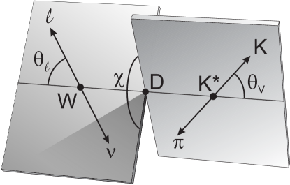
Figure 1: Definition of kinematic variables.

The full intensity distribution for $D^{+}\rightarrow K^{-}\pi^{+}\mu^{+}\nu$, differential in these five kinematic variables, is given in Reference [2]. Throughout this paper, we will use the simpler expression given by Eq. LABEL:amp1 that gives the form of this decay intensity after integration over the acoplanarity angle $\chi$. The $\chi$ integration significantly simplifies the intensity by eliminating all interference terms between different helicity states of the virtual $W^{+}$ with relatively little loss in form factor information. Following the notation of [1], the Eq. LABEL:amp1 intensity is written in terms of the four helicity basis form factors: $H_{+}(q^{2}),H_{0}(q^{2}),H_{-}(q^{2}),H_{t}(q^{2})$ along with an additional form factor $h(q^{2})$ that describes the coupling of an additional, small $s$-wave amplitude contribution (with a constant amplitude $Ae^{i\delta}$) that is discussed in Reference [4]. Our earlier papers [4, 2] assumed that the s-wave amplitude had the same zero helicity form factor as that for $D^{+}\rightarrow\overline{K}^{*0}\mu^{+}\nu$ – e.g. $h_{0}(q^{2})=H_{0}(q^{2})$. The acoplanarity averaged intensity in terms of the decay angles, helicity form factor products, and $\overline{K}^{*0}$ Breit-Wigner amplitude ($BW$) is:

$$\int{|A|^{2}d\chi}=\frac{q^{2}-m_{\ell}^{2}}{8}\left\{\begin{array}[]{l}((1+\cos\theta_{\ell})\sin\theta_{\textrm{v}})^{2}|H_{+}(q^{2})|^{2}|\textrm{BW}|^{2}\\ +((1-\cos\theta_{\ell})\sin\theta_{\textrm{v}})^{2}|H_{-}(q^{2})|^{2}|\textrm{BW}|^{2}\\ +(2\sin\theta_{\ell}\cos\theta_{\textrm{v}})^{2}|H_{0}(q^{2})|^{2}|\textrm{BW}|^{2}\\ +8\sin^{2}\theta_{\ell}\cos\theta_{\textrm{v}}H_{0}(q^{2})h_{o}(q^{2}){\mathop{\rm Re}\nolimits}\{Ae^{-i\delta}\textrm{BW}\}\end{array}\right\}$$ (5)

(6)

$$\mbox{}+\frac{|\textrm{BW}|^{2}}{8}(q^{2}-m_{\ell}^{2})\frac{m_{\ell}^{2}}{q^{2}}\left\{\begin{array}[]{l}(\sin\theta_{\ell}\sin\theta_{\textrm{v}})^{2}|H_{+}|^{2}+(\sin\theta_{\ell}\sin\theta_{\textrm{v}})^{2}|H_{-}|^{2}\\ +(2\cos\theta_{\ell}\cos\theta_{\textrm{v}})^{2}|H_{0}|^{2}\\ +(2\cos\theta_{\textrm{v}})^{2}|H_{t}|^{2}+8\cos\theta_{\ell}\cos^{2}\theta_{\textrm{v}}H_{0}H_{t}\end{array}\right\}\,,$$ (10)

where

$$\textrm{BW}=\frac{\sqrt{m_{0}\Gamma}\left(\frac{P^{*}}{P_{0}^{*}}\right)}{m_{K\pi}^{2}-m_{0}^{2}+im_{0}\Gamma\left(\frac{P^{*}}{P_{0}^{*}}\right)^{3}}\,.$$ (11)

The first term gives the intensity for the $\mu^{+}$ to be right-handed, while the (highly suppressed) second term gives the intensity for it to be left-handed.

Before describing the non-parametric approach, we begin with a description of the traditional experimental approach. The $D^{+}\rightarrow\overline{K}^{*0}\mu^{+}\nu$ decay amplitude is typically analyzed [1] in terms of four form factors. This intensity expression is written in terms of four helicity basis form factors that are in turn written as linear combinations of vector and axial form factors as given in Eq. 12.

$$H_{\pm}(q^{2}) = (M_{D}+m_{K\pi})A_{1}(q^{2})\mp 2{M_{D}K\over M_{D}+m_{K\pi}}V(q^{2})\,,$$

$$H_{0}(q^{2}) = {1\over 2m_{K\pi}\sqrt{q^{2}}}\left[(M^{2}_{D}-m^{2}_{K\pi}-q^{2})(M_{D}+m_{K\pi})A_{1}(q^{2})\frac{}{}\right.$$ (12)

$$\mbox{}\hskip 56.9055pt\left.-4{M^{2}_{D}K^{2}\over M_{D}+m_{K\pi}}A_{2}(q^{2})\right]\,,$$

$$H_{t}(q^{2}) = {M_{D}K\over m_{K\pi}\sqrt{q^{2}}}\left[(M_{D}+m_{K\pi})A_{1}(q^{2})-{(M^{2}_{D}-m^{2}_{K\pi}+q^{2})\over M_{D}+m_{K\pi}}A_{2}(q^{2})\right.$$

$$\mbox{}\hskip 56.9055pt\left.+{2q^{2}\over M_{D}+m_{K\pi}}A_{3}(q^{2})\right]\,,$$

where $K$ is the momentum of the $K^{-}\pi^{+}$ system in the rest frame of the $D^{+}$. The vector and axial form factors are generally parameterized by a pole dominance form:

$$A_{i}(q^{2})={A_{i}(0)\over 1-q^{2}/M_{A}^{2}}~{}~{}~{}~{}\textrm{and}~{}~{}~{}~{}V(q^{2})={V(0)\over 1-q^{2}/M_{V}^{2}}\,,$$ (13)

where all previous experiments used spectroscopic pole masses of $M_{A}=2.5~{}\textrm{GeV}/c^{2}$ and $M_{V}=2.1~{}\textrm{GeV}/c^{2}$ which in the case of $D^{+}\rightarrow\overline{K}^{*0}\mu^{+}\nu$ are tied to masses of vector and axial $D_{s}^{*}$ states.

Using the spectroscopic pole dominance assumption, previous experiments [2, 3] have fit the shape of the $D^{+}\rightarrow\overline{K}^{*0}\mu^{+}\nu$ intensity to at most 3 parameters which are ratios of form factors taken at $q^{2}=0$ : $r_{v}\equiv V(0)/A_{1}(0),\ r_{2}\equiv A_{2}(0)/A_{1}(0),\ r_{3}\equiv A_{3}(0)/A_{1}(0)$ and in one case [2] the (constant) $s$-wave complex amplitude.

As in our earlier paper [5] on the $q^{2}$ dependence of the $D^{0}\rightarrow K^{-}\mu^{+}\nu$ form factor, we present the first non-parametric measurements of the helicity basis form factors that describe $D^{+}\rightarrow K^{-}\pi^{+}\mu^{+}\nu$ decay. In particular, we will provide information on $H_{\pm}^{2}(q^{2})$, $H_{0}^{2}(q^{2})$, and $h_{0}(q^{2})\times H_{0}(q^{2})$ in bins of $q^{2}$ by projecting out the associated angular factors given in Eq. LABEL:amp1. The cross term $h_{0}(q^{2})\times H_{0}(q^{2})$ represents the interference between the $s$-wave and the $K^{*0}$.

Throughout this paper, unless explicitly stated otherwise, the charge conjugate is also implied when a decay mode of a specific charge is stated.

2 Experimental and analysis details

The data for this paper were collected in the Wideband photoproduction experiment FOCUS during the Fermilab 1996–1997 fixed-target run. In FOCUS, a forward multi-particle spectrometer is used to measure the interactions of high energy photons on a segmented BeO target. The FOCUS detector is a large aperture, fixed-target spectrometer with excellent vertexing and particle identification. The FOCUS experiment and analysis techniques have been described previously [4, 6, 7].

To isolate the $D^{+}\rightarrow K^{-}\pi^{+}\mu^{+}\nu$ topology, we required that candidate muon, pion, and kaon tracks formed a secondary vertex with a confidence level exceeding 25%. We required a primary vertex consisting of at least two charged tracks. The muon track, when extrapolated to the shielded muon arrays, was required to match muon hits with a confidence level exceeding 5%. The kaon was required to have a Čerenkov light pattern more consistent with that for a kaon than that for a pion by 1 unit of log likelihood [7]. No Čerenkov requirement was made on the pion.

To further reduce muon misidentification, a muon candidate was allowed to have at most one missing hit in the 6 planes comprising our inner muon system and a momentum exceeding 10 GeV$/c$. In order to suppress muons from pions and kaons decaying within our apparatus, we required that each muon candidate had a confidence level exceeding 2% to the hypothesis that it had a consistent trajectory through our two analysis magnets.

Non-charm and random combinatoric backgrounds were reduced by requiring both a detachment between the vertex containing the $K^{-}\pi^{+}\mu^{+}$ and the primary production vertex of at least 10 standard deviations and a minimum visible energy $(E_{K}+E_{\pi}+E_{\mu})$ of 30 GeV. To suppress possible backgrounds from higher multiplicity charm decays, we isolate the $K\pi\mu$ vertex from other tracks in the event (not including tracks in the primary vertex) by requiring that the maximum confidence level for another track to form a vertex with the candidate be less than 0.1%.

In order to allow for the missing energy of the neutrino in this semileptonic $D^{+}$ decay, we required the reconstructed $K\pi\mu$ mass be less than the nominal $D^{+}$ mass. Background from $D^{+}\rightarrow K^{-}\pi^{+}\pi^{+}$, where a pion is misidentified as a muon, was reduced using a mass cut: we required that when the muon track is treated as a pion and the combination is reconstructed as a $K\pi\pi$, the $K\pi\pi$ invariant mass was less than 1.820 $\textrm{GeV}/c^{2}$. In order to suppress background from $D^{*+}\rightarrow D^{0}\pi^{+}\rightarrow(K^{-}\mu^{+}\nu)\pi^{+}$, we required $M(K^{-}\mu^{+}\nu\pi^{+})-M(K^{-}\mu^{+}\nu)>0.18~{}\textrm{GeV}/c^{2}$. The wrong-sign subtracted $m_{K\pi}$ distribution for these $D^{+}\rightarrow K^{-}\pi^{+}\mu^{+}\nu$ candidates is shown in Figure 2. Wrong-sign events have tracks identified as $K^{-}\pi^{+}\mu^{-}$ isolated in a detached vertex.

Figure 2: Wrong-sign subtracted $D^{+}\rightarrow K^{-}\pi^{+}\mu^{+}\nu$ signal. Over the full displayed mass range there is a right-sign excess of 14 798 events. For this analysis, we use a restricted mass range from 0.846–0.946 $\textrm{GeV}/c^{2}$ (shown by vertical lines). In this restricted region, there is a right-sign excess of 11 397 events.

We will use a restricted mass range from 0.846–0.946 $\textrm{GeV}/c^{2}$ in this analysis in an effort to diminish the dependence of the helicity basis form factors on $m_{K\pi}$ through Eq. 12.

The technique used to reconstruct the neutrino momentum through the $D^{+}$ line-of-flight and tests of our ability to simulate the resolution on kinematic variables that rely on the neutrino momentum are described in Reference [4].

3 Projection Weighting Technique

In this section, we describe the weighting technique that we use to extract the helicity basis form factors that describe the $D^{+}\rightarrow K^{-}\pi^{+}\mu^{+}\nu$ angular distribution according to Eq. LABEL:amp1. For a given $q^{2}$ bin, a weight will be assigned to the event depending on its $\theta_{\textrm{v}}$ and $\theta_{\ell}$ decay angle. We consider 25 joint $\Delta\cos\theta_{\textrm{v}}\times\Delta\cos\theta_{\ell}$ angular bins: 5 evenly spaced bins in $\cos\theta_{\textrm{v}}$ times 5 bins in $\cos\theta_{\ell}$. Each event will acquire a weight designed to project out a given helicity form factor that depends on which of the 25 angular bins that it is reconstructed in. It is convenient to think of weighting as constructing a dot product of the form $\vec{P}_{\alpha}\cdot\vec{D}$ where $\vec{D}$ is a data vector that consists of the number of events reconstructed in each of the 25 angular vectors $\vec{D}=({\begin{array}[]{*{20}c}{n_{1}}&{n_{2}}&{...}&{n_{25}}\\ \end{array}})$ and $\vec{P}_{\alpha}$ is a projection vector for the $\alpha$ helicity form factor. The 25 components of each $\vec{P}_{\alpha}$ vector give the weights applied to each event reconstructed in one of the 25 angular bins. Eq. 14 says the product $\vec{P}_{+}\cdot\vec{D}$ is equivalent to weighting the events in angular bin 1 by $\left[\vec{P}_{+}\right]_{1}$, weighting the events in angular bin 2 by $\left[\vec{P}_{+}\right]_{2}$, etc.

$$\vec{P}_{+}\cdot\vec{D}=\left[\vec{P}_{+}\right]_{1}n_{1}+\left[\vec{P}_{+}\right]_{2}n_{2}+\cdots\left[\vec{P}_{+}\right]_{25}n_{25}\,.$$ (14)

The $\vec{P}_{\alpha}$ weights are designed to project out the helicity form factors using Monte Carlo inputs. Here is how they are obtained. To simplify our discussion, consider the case of just three form factors $H_{+}^{2}(q^{2})$, $H_{-}^{2}(q^{2})$, $H_{0}^{2}(q^{2})$. For each $q^{2}_{i}$ bin, let $\{\vec{m}_{\alpha}\}=({\begin{array}[]{*{20}c}{\vec{m}_{+}}&{\vec{m}_{-}}&{\vec{m}_{0}}\end{array}})$ where $\vec{m}_{\alpha}$ is the number of events present in each of the 25 angular bins when a nominal $H_{\alpha}(q_{i}^{2})$ is turned on and all other nominal $H_{\alpha\neq\beta}(q_{i}^{2})$ are turned off. As indicated in Eq. 15, for each $q^{2}_{i}$ bin the $\vec{D}_{i}$ vector can be written as a linear combination of the three $\vec{m}$ vectors with coefficients $f_{\alpha}(q_{i}^{2})$. The $f_{\alpha}(q_{i}^{2})$ functions are proportional to the true $H^{2}_{\alpha}(q_{i}^{2})$ along with pre-factors such as $q^{2}-m_{\ell}^{2}$ and corrections such as acceptance and resolution.

$$\vec{D}_{i}=f_{+}(q_{i}^{2})\>\vec{m}_{+}+f_{-}(q_{i}^{2})\>\vec{m}_{-}+f_{0}(q_{i}^{2})\>\vec{m}_{0}\,.$$ (15)

We can convert Eq. 15 to the “component equation” shown in Eq. 16.

$$\left({\begin{array}[]{*{20}c}{\vec{m}_{+}\cdot\vec{D}_{i}}\\ {\vec{m}_{-}\cdot\vec{D}_{i}}\\ {\vec{m}_{0}\cdot\vec{D}_{i}}\\ \end{array}}\right)=\left({\begin{array}[]{*{20}c}{\vec{m}_{+}\cdot\vec{m}_{+}}&{\vec{m}_{+}\cdot\vec{m}_{-}}&{\vec{m}_{+}\cdot\vec{m}_{0}}\\ {\vec{m}_{-}\cdot\vec{m}_{+}}&{\vec{m}_{-}\cdot\vec{m}_{-}}&{\vec{m}_{-}\cdot\vec{m}_{0}}\\ {\vec{m}_{0}\cdot\vec{m}_{+}}&{\vec{m}_{0}\cdot\vec{m}_{-}}&{\vec{m}_{0}\cdot\vec{m}_{0}}\\ \end{array}}\right)\left({\begin{array}[]{*{20}c}{f_{+}(q_{i}^{2})}\\ {f_{-}(q_{i}^{2})}\\ {f_{0}(q_{i}^{2})}\\ \end{array}}\right)\,.$$ (16)

The solution to Eq. 16 can be written as:

$$f_{+}(q_{i}^{2})={}^{i}\vec{P}_{+}\cdot\vec{D}_{i}\,,\ f_{-}(q_{i}^{2})={}^{i}\vec{P}_{-}\cdot\vec{D}_{i}\,,\ f_{0}(q_{i}^{2})={}^{i}\vec{P}_{0}\cdot\vec{D}_{i}\,,$$ (17)

where our notation is that the left superscript gives the $q^{2}$ bin number and the subscript identifies the helicity of the projector.

The ${}^{i}\vec{P}_{\alpha}$ weights are given by Eq. 18.

$$\left({\begin{array}[]{*{20}c}{{}^{i}\vec{P}_{+}}\\ {{}^{i}\vec{P}_{-}}\\ {{}^{i}\vec{P}_{0}}\\ \end{array}}\right)=\left({\begin{array}[]{*{20}c}{\vec{m}_{+}\cdot\vec{m}_{+}}&{\vec{m}_{+}\cdot\vec{m}_{-}}&{\vec{m}_{+}\cdot\vec{m}_{0}}\\ {\vec{m}_{-}\cdot\vec{m}_{+}}&{\vec{m}_{-}\cdot\vec{m}_{-}}&{\vec{m}_{-}\cdot\vec{m}_{0}}\\ {\vec{m}_{0}\cdot\vec{m}_{+}}&{\vec{m}_{0}\cdot\vec{m}_{-}}&{\vec{m}_{0}\cdot\vec{m}_{0}}\\ \end{array}}\right)^{-1}\left({\begin{array}[]{*{20}c}{\vec{m}_{+}}\\ {\vec{m}_{-}}\\ {\vec{m}_{0}}\\ \end{array}}\right)\,.$$ (18)

One can correct for acceptance by using the proportionality relations such as Eq. 19,

$$f_{i}^{+}={}^{i}\vec{P}_{+}\cdot\vec{D}_{i}=\frac{(H_{+}(q_{i}^{2}))^{2}}{(\tilde{H}_{i}^{+})^{2}}\>{}^{i}\vec{P}_{+}\cdot\vec{M}_{i}$$

$$\Rightarrow(H_{+}(q_{i}^{2}))^{2}=\left[\frac{({}^{i}\tilde{H}_{+})^{2}}{{}^{i}\vec{P}_{+}\cdot\vec{M}_{i}}\>\>{}^{i}\vec{P}_{+}\right]\cdot\vec{D}_{i}\equiv{}^{i}\rho_{+}\cdot\vec{D}_{i}\,,$$ (19)

where $\vec{M}_{i}$ are the bin populations from a Monte Carlo, generated assuming a trial form factor set $\tilde{H}_{+}^{2}(q^{2})$, $\tilde{H}_{-}^{2}(q^{2})$, and $\tilde{H}_{0}^{2}(q^{2})$. As indicated in Eq. 19, the projection weights ${}^{i}\vec{P}_{+}$ and the projection-weighted Monte Carlo distributions (${}^{i}\vec{P}_{+}\cdot\vec{M}_{i}$) can then be used to construct an adjusted weight vector ${{}^{i}\vec{\rho}}_{+}$. The (arbitrarily normalized) form factors $H_{+}^{2}(q^{2})$, $H_{-}^{2}(q^{2})$ and $H_{0}^{2}(q^{2})$ would then be obtained by making three weighted histograms using the ${{}^{i}\vec{\rho}}_{+}$, ${{}^{i}\vec{\rho}}_{-}$ and ${{}^{i}\vec{\rho}}_{0}$ weights respectively.

We next discuss some of the complications in applying the projective weighting scheme in our experiment due to smearing of kinematic variables because of the missing neutrino. In the absence of substantial $q^{2}$ smearing, a totally arbitrary set of trial form factors (such as $\tilde{H}_{\alpha}(q^{2}_{i})=1$) can be used to get unbiased estimates of the helicity basis form factors. This is no longer true when smearing in the kinematic variables $q^{2},\ \cos\theta_{\textrm{v}},\ \cos\theta_{\ell}$ is substantial since one must use reconstructed quantities in dealing with the data. The acceptance and resolution that affect the ${{}^{i}\vec{\rho}}_{+}$, ${{}^{i}\vec{\rho}}_{-}$ and ${{}^{i}\vec{\rho}}_{0}$ weights depend on the true kinematic variables. Since the mapping between the true kinematic variables and reconstructed kinematic variables depends on the underlying form factors, one can bias the returned form factors to the extent that $\tilde{H}_{\alpha}(q^{2}_{i})\neq H_{\alpha}(q^{2}_{i})$. We found through Monte Carlo simulation that it is only important to get a reasonably good first guess for $\tilde{H}_{\alpha}(q^{2}_{i})$ and multiple iteration is not required given the size of our statistical error bars.

Although the mass terms of Eq. LABEL:amp1 are suppressed by two powers of the muon mass, they are surprisingly important at low $q^{2}$. Our analysis includes projectors for each of the six form factor products present in Eq. LABEL:amp1. Although we were unable to obtain useful information on $H^{2}_{t}(q^{2})$ or the $H_{0}(q^{2})\times H_{t}(q^{2})$ interference term, we needed to allow for them in the construction of ${}^{i}\vec{P}_{\alpha}$ using Eq. 18 to insure that the projectors used for $H_{\pm}^{2}(q^{2})$, $H_{0}^{2}(q^{2})$, and $h_{0}(q^{2})\times H_{0}(q^{2})$ will be “orthogonal” to the angular terms associated with the $H^{2}_{t}(q^{2})$ and $H_{0}(q^{2})\times H_{t}(q^{2})$ contributions of Eq. LABEL:amp1. Without the incorporation of the mass term projectors, we see a dramatic mismatch between the input and output form factors for $H_{\pm}^{2}(q^{2})$ in the first $q^{2}$ bin in our Monte Carlo studies. For example, $H_{-}^{2}(q^{2})$ nearly drops to zero in the first $q^{2}$ bin if projectors for the mass terms are not included.

Figure 3 summarizes a complete Monte Carlo simulation of the projective weighting technique. This Monte Carlo was run with 9 times our data sample but we have inflated the error bars by a factor of three to indicate the estimate of the errors expected in the data. The form factor measurements are plotted at the abscissa of the average generated $q^{2}$ for each of the 6 evenly spaced measured $q^{2}$ bins rather than at the measured bin center. The good agreement between the input and output form factors validates our assumption that the $|A|^{2}$ term can be dropped when constructing the projective weights since these terms are included in the Monte Carlo simulation.

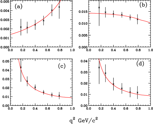
Figure 3: Monte Carlo study of the projective weighting technique. The form factors used in this Monte Carlo simulation are shown as the solid curves. The reconstructed form factors are the points with error bars. They are plotted in “arbitrary” units but the same unit is used for all four form factors in order to convey the relative size of each contribution. The plots are: (a) $H_{+}^{2}(q^{2})$, (b) $H_{-}^{2}(q^{2})$, (c) $H_{0}^{2}(q^{2})$, and (d) $h_{0}(q^{2})\times H_{0}(q^{2})$.

The method does an excellent job at reproducing the input form factor products (shown as a curve) both in terms of the shape and relative contribution from each of the 4 form factor products. The input form factors used the measurements and $s$-wave model developed in Reference [2].

Figure 4 and Table 1 show the results obtained for data. The form factor measurements are plotted at the abscissa of the average generated $q^{2}$ for each of the 6 evenly spaced measured $q^{2}$ bins as determined from the Monte Carlo. The horizontal error bars given the r.m.s $q^{2}$ resolution for each bin. We have subtracted the weighted distribution obtained for background events simulated in our charm Monte Carlo that incorporates all known charm decays. Non-charm backgrounds are primarily eliminated through a wrong-sign subtraction. Applying more stringent cuts in the analysis indicates that the only significant deviation from the model occurs in plot a) of Fig. 4 in the lowest bin. While we believe the low bin in $H_{+}(q^{2})$ represents a very small fraction of the cross section for the decay and is, hence, particularly susceptible to unanticipated backgrounds, we cannot rule out that this effect originates in the physics of the real decay.

We will refer to this representation of the data as the un-convolved analysis since the vertical error bars in Figure 4 do not represent the uncertainty in the form factors averaged within each bin boundary. This is because we have not corrected for the considerable smearing between the various $q^{2}$ bins by using the deconvolution technique [5] discussed in the next section. To the extent that the form factors vary smoothly, the un-convolved representation should still be faithful to the underlying form factors as was the case of the Monte Carlo study shown in Figure 3. We include the un-convolved results since they show more $q^{2}$ bins than possible in our deconvolution analysis discussed in the next section.

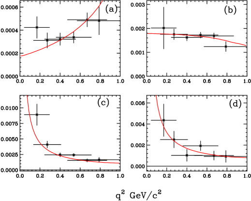
Figure 4: Non-parametric form factors obtained for data with horizontal error bars given by our r.m.s. resolution. The plots are: (a) $H_{+}^{2}(q^{2})$, (b) $H_{-}^{2}(q^{2})$, (c) $H_{0}^{2}(q^{2})$, and (d) $h_{0}(q^{2})\times H_{0}(q^{2})$. The r.m.s $q^{2}$ resolution varies (monotonically) from 0.125 $\textrm{GeV}^{2}/c^{4}$, in the first bin, to 0.218 $\textrm{GeV}^{2}/c^{4}$ in the last bin.

Table 1: Summary of un-convolved results. This is a tabular summary of the data of Fig. 4 multiplied by 1000.

$q^{2}$	$q^{2}{}_{rms}$	$H_{+}^{2}$	$H_{-}^{2}$	$H_{0}^{2}$	$h_{0}\times H_{0}$
0.169	0.125	0.42 $\pm$ 0.09	2.02 $\pm$ 0.87	8.91 $\pm$ 1.71	4.36 $\pm$ 1.53
0.272	0.136	0.31 $\pm$ 0.07	1.75 $\pm$ 0.22	4.09 $\pm$ 0.54	2.53 $\pm$ 0.78
0.400	0.154	0.32 $\pm$ 0.05	1.62 $\pm$ 0.14	2.44 $\pm$ 0.32	1.03 $\pm$ 0.57
0.536	0.175	0.34 $\pm$ 0.05	1.72 $\pm$ 0.12	2.40 $\pm$ 0.24	1.93 $\pm$ 0.46
0.670	0.196	0.49 $\pm$ 0.06	1.68 $\pm$ 0.12	1.54 $\pm$ 0.24	1.01 $\pm$ 0.42
0.789	0.218	0.48 $\pm$ 0.12	1.24 $\pm$ 0.20	1.64 $\pm$ 0.40	0.92 $\pm$ 0.56

4 Deconvolution Weighting

Because of $q^{2}$ smearing, the sum of the $\vec{P}_{+}$ weights in a given reconstructed $q^{2}$ bin will depend on both the underlying $H^{2}_{+}({}^{1}q^{2})$ for that bin as well as the underlying $H^{2}_{+}({}^{i\neq 1}q^{2})$ form factor for all other bins. Hence the old Eq. 19 correction becomes the non-local version given by Eq. 20 where for notational simplicity we just consider two $q^{2}$ bins.

$$f_{+}({}^{1}q^{2})={}^{1}\vec{P}_{+}\cdot{}^{1}\vec{D}={}^{1}w_{1}\frac{H_{+}^{2}(q_{1}^{2})}{(\tilde{H}_{1}^{+})^{2}}+{}^{1}w_{2}\frac{H_{+}^{2}(q_{2}^{2})}{(\tilde{H}_{2}^{+})^{2}}\,,$$ (20)

where ${}^{1}w_{1}={}^{1}\vec{P}_{+}\cdot{}^{1}\vec{M}_{1}$ is the sum of the Monte Carlo weights that reconstruct in $q^{2}$ bin 1 when generated in $q^{2}$ bin 1 and ${}^{1}w_{2}={}^{1}\vec{P}_{+}\cdot{}^{1}\vec{M}_{2}$ is the sum of the Monte Carlo weights that reconstruct in $q^{2}$ bin 1 when generated in $q^{2}$ bin 2. Eq. 20 can be generalized to Eq. 21.

$$\left({\begin{array}[]{*{20}c}{f_{+}({}^{1}q^{2})}\\ {f_{+}({}^{2}q^{2})}\\ \end{array}}\right)=\left({\begin{array}[]{*{20}c}{{}^{1}\vec{P}_{+}\cdot{}^{1}\vec{D}}\\ {{}^{2}\vec{P}_{+}\cdot{}^{2}\vec{D}}\\ \end{array}}\right)=\left({\begin{array}[]{*{20}c}{\frac{{}^{1}w_{1}}{(\tilde{H}_{1}^{+})^{2}}}&{\frac{{}^{1}w_{2}}{(\tilde{H}_{2}^{+})^{2}}}\\ {\frac{{}^{2}w_{1}}{(\tilde{H}_{1}^{+})^{2}}}&{\frac{{}^{2}w_{2}}{(\tilde{H}_{2}^{+})^{2}}}\\ \end{array}}\right)\left({\begin{array}[]{*{20}c}{H_{+}^{2}(q_{1}^{2})}\\ {H_{+}^{2}(q_{2}^{2})}\\ \end{array}}\right)\,.$$ (21)

The solution to Eq. 21 is given by Eq. 22.

$$\left({\begin{array}[]{*{20}c}H_{+}^{2}(q_{1}^{2})\\ H_{+}^{2}(q_{2}^{2})\\ \end{array}}\right)=\left({\begin{array}[]{*{20}c}{\frac{{}^{1}w_{1}}{(\tilde{H}_{1}^{+})^{2}}}&{\frac{{}^{1}w_{2}}{(\tilde{H}_{2}^{+})^{2}}}\\ {\frac{{}^{2}w_{1}}{(\tilde{H}_{1}^{+})^{2}}}&{\frac{{}^{2}w_{2}}{(\tilde{H}_{2}^{+})^{2}}}\\ \end{array}}\right)^{-1}\left({\begin{array}[]{*{20}c}{{}^{1}\vec{P}_{+}\cdot{}^{1}\vec{D}}\\ {{}^{2}\vec{P}_{+}\cdot{}^{2}\vec{D}}\\ \end{array}}\right)\,.$$ (22)

This solution is equivalent to weighting the data using the weights given by Eq. 23.

$$\left({\begin{array}[]{*{20}c}{\vec{\rho}_{1}^{+}}\\ {\vec{\rho}_{2}^{+}}\\ \end{array}}\right)=\left({\begin{array}[]{*{20}c}{\frac{{}^{1}w_{1}}{(\tilde{H}_{1}^{+})^{2}}}&{\frac{{}^{1}w_{2}}{(\tilde{H}_{2}^{+})^{2}}}\\ {\frac{{}^{2}w_{1}}{(\tilde{H}_{1}^{+})^{2}}}&{\frac{{}^{2}w_{2}}{(\tilde{H}_{2}^{+})^{2}}}\\ \end{array}}\right)^{-1}\left({\begin{array}[]{*{20}c}{{}^{1}\vec{P}_{+}}\\ {{}^{2}\vec{P}_{+}}\\ \end{array}}\right)\,.$$ (23)

In order to obtain $H_{+}^{2}(q_{1}^{2})$, for example, one weights each event by $\vec{\rho}_{1}^{+}$. By Eq. 23, $\vec{\rho}_{1}^{+}$ is constructed from a sum of the vector ${}^{1}\vec{P}_{+}$ that contains the angular weights for events that reconstruct in $q^{2}$ bin 1 and the vector ${}^{2}\vec{P}_{+}$ that contains the angular weights for events that reconstruct in $q^{2}$ bin 2.

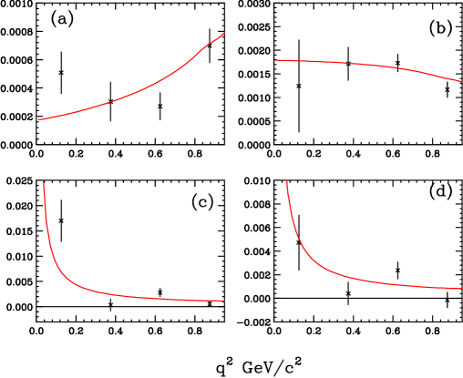
Figure 5: Non-parametric form factors obtained for deconvolved data. The plots are: (a) $H_{+}^{2}(q^{2})$, (b) $H_{-}^{2}(q^{2})$, (c) $H_{0}^{2}(q^{2})$, and (d) $h_{0}(q^{2})\times H_{0}(q^{2})$.

Table 2: Summary of deconvolved results. This is a tabular summary of the data of Fig. 5 multiplied by 1000.

$q^{2}$	$H_{+}^{2}$	$H_{-}^{2}$	$H_{0}^{2}$	$h_{0}\times H_{0}$
0.125	0.508 $\pm$ 0.15	1.24 $\pm$ 0.97	17.00 $\pm$ 4.05	4.72 $\pm$ 2.33
0.375	0.304 $\pm$ 0.14	1.71 $\pm$ 0.35	0.33 $\pm$ 1.17	0.41 $\pm$ 0.95
0.625	0.270 $\pm$ 0.10	1.73 $\pm$ 0.18	2.82 $\pm$ 0.82	2.37 $\pm$ 0.71
0.875	0.698 $\pm$ 0.12	1.16 $\pm$ 0.16	0.54 $\pm$ 0.49	-0.14 $\pm$ 0.65

Figure 5 and Table 2 show the result of a four $q^{2}$ bin deconvolution of the data. Only four bins are used since as the $q^{2}$ smearing exceeds the bin separation the “resolution” matrix that is inverted in Eq. 23 becomes increasingly more singular resulting in greatly inflated error bars as well as strong negative correlations appearing between adjacent bins [5]. Essentially the same features that appear in the un-convolved representation of the data seen in Figure 4 appear in Figure 5 but on a coarser scale. There is a small overshoot in the first bin of both $H^{2}_{+}$ and $H^{2}_{0}$, but generally both the shape and relative normalization of the form factors are a reasonable match to the model of Reference [2].

We have estimated systematic errors by studying the stability of the results to changes in the number of angular bins, changes in the analysis cuts, and changes in our assumed background level. For the three form factor products describing the $D^{+}\rightarrow\overline{K}^{*0}\mu^{+}\nu$ component – $H_{+}^{2}(q^{2})$, $H_{-}^{2}(q^{2})$, and $H_{0}^{2}(q^{2})$ – the systematic errors are estimated to be less than 20% of the statistical error apart from the first $q^{2}$ bin for $H^{2}_{+}(q^{2}{})$, where we assess a systematic error equal to the statistical error. This first $q^{2}$ bin also requires a large ($\approx 30\%$) background subtraction. For the $h_{0}(q^{2})\times H_{0}(q^{2})$ form factor product describing the s-wave interference we assess a systematic error equal to 30% of the statistic error. The background subtraction for the $h_{0}(q^{2})\times H_{0}(q^{2})$ form factor product is also large ($\approx 50\%$) for the first three $q^{2}{}$ bins. The errors quoted in Tables 1 and 2 do not include these systematic errors.

5 Summary

We presented the first non-parametric analysis of the helicity basis form factors that control the decay $D^{+}\rightarrow K^{-}\pi^{+}\mu^{+}\nu$. We used a projective weighting technique that allows one to determine the helicity form factor products by weighted histograms rather than likelihood based fits. This method should prove to be a valuable technique for the $e^{+}e^{-}$ charm factories that have much better $q^{2}$ resolution. The non-parametric technique can also be used for other four body semileptonic decays like $D^{+}\rightarrow\rho\;\ell^{+}\nu_{\ell}$ and $D_{s}^{+}\rightarrow\phi\;\ell^{+}\nu_{\ell}$. We presented both an un-convolved and deconvolved representation of the data. Both representations were a reasonable match to the spectroscopic pole dominance assumption with form factor ratios given in [2]. The $q^{2}$ dependence of the form factor governing the $s$-wave contribution to $D^{+}\rightarrow K^{-}\pi^{+}\mu^{+}\nu$ is also studied for the first time. We find that the shape of the $s$-wave form factor ($h_{0}(q^{2})$) is reasonably consistent with the $H_{0}(q^{2})$ form factor as assumed in Reference [2].

6 Acknowledgments

We wish to acknowledge the assistance of the staffs of Fermi National Accelerator Laboratory, the INFN of Italy, and the physics departments of the collaborating institutions. This research was supported in part by the U. S. National Science Foundation, the U. S. Department of Energy, the Italian Istituto Nazionale di Fisica Nucleare and Ministero dell’Università e della Ricerca Scientifica e Tecnologica, the Brazilian Conselho Nacional de Desenvolvimento Científico e Tecnológico, CONACyT-México, the Korean Ministry of Education, and the Korean Science and Engineering Foundation.

References

[1]
J.G. Korner and G.A. Schuler, Z. Phys. C 46 (1990) 93.
[2]
FOCUS Collab., J.M. Link et al., Phys. Lett. B 544 (2002) 89.
[3]
BEATRICE Collab., M. Adamovich et al., Eur. Phys. J. C 6 (1999) 35.
E791 Collab., E. M. Aitala et al., Phys. Rev. Lett. 80 (1998) 1393.
E791 Collab., E. M. Aitala et al., Phys. Lett. B 440 (1998) 435.
E687 Collab., P.L. Frabetti et al., Phys. Lett. B 307 (1993) 262.
E653 Collab., K. Kodama et al., Phys. Lett. B 274 (1992) 246.
E691 Collab., J. C. Anjos et al., Phys. Rev. Lett. 65 (1990) 2630.
[4]
FOCUS Collab., J.M. Link et al., Phys. Lett. B 535 (2002) 43.
[5]
FOCUS Collab., J.M. Link et al., Phys. Lett. B 607 (2004) 233.
[6] E687 Collab., P. L. Frabetti et al.,
Nucl. Instrum. Methods A 320 (1992) 519.
[7]FOCUS Collab., J. M. Link et al., Nucl. Instrum. Methods A 484
(2002) 270.