Charm meson spectra in $e^{+}e^{-}$ annihilation at 10.5 GeV c.m.e.

Abstract

Using the CLEO detector at the Cornell Electron-positron Storage Ring, we have measured the scaled momentum spectra, $d\sigma/dx_{p}$, and the inclusive production cross sections of the charm mesons $D^{+}$, $D^{0}$, $D^{\star+}$ and $D^{\star 0}$ in $e^{+}e^{-}$ annihilation at about 10.5 GeV center of mass energy, excluding the decay products of B mesons. The statistical accuracy and momentum resolution are superior to previous measurements at this energy.

I Introduction

We report the measurement of the momentum spectra of charged and neutral $D$ and $D^{*}$ charm mesons produced at the Cornell Electron-positron Storage Ring, CESR, in non-resonant $e^{+}e^{-}$ annihilation at about 10.5 GeV center of mass energy (CME) and observed with the CLEO detector. The $D^{0}$ and $D^{+}$ spectra each include both directly produced $D$’s, and $D$’s which are decay products of $D$ excited states. From them we also derive the inclusive production cross section for these charm mesons.

While very accurate data on bottom quark production from LEP and SLD have been published in recent years Alexander:1995aj ; Abe:1999ki ; Heister:2001jg ; Adeva:1991iw , the data currently available for studies of charm fragmentation at 10.5 GeV CME Argus91 ; CLEO88 , are quite old and, by present standards, of poor statistical quality and momentum resolution. Our statistical sample is about 80 times larger than the our previous one CLEO88 and our current momentum resolution is about a factor of 2 better.

The spectra represent measurements of charm quark fragmentation distributions $D^{h}_{c}(x,s)$, i.e., the probability density that a $c$ quark produces a charm hadron $h$ carrying a fraction $x$ of its momentum, $\sqrt{s}$ being the “energy scale” of the process, the $e^{+}e^{-}$ CME in our case biebel ; Nason:1993xx . Experimental heavy-meson spectra in $e^{+}e^{-}$ collisions are important for theoretical and practical reasons: (i) they provide a component that is not yet calculable in predicting heavy flavor production in very high energy hadronic collisions, (ii) they can test advanced perturbative QCD (PQCD) methods, (iii) they can test the QCD evolution equations, and (iv) they provide information for best parametrization of the Monte Carlo simulations on which the analysis of many high energy experiments partially rely.

Items (i) and (ii) are interconnected. The calculations of heavy flavor production cross sections in hadronic collisions (e.g., at the Tevatron and the LHC) are generally based on the factorization hypothesis, i.e., a convolution of (a) the parton distribution function for the colliding hadrons, (b) the perturbative calculation of the parton-parton cross section and (c) the parton fragmentation function $D^{h}_{q}(x,s)$. Items (b) and part of (c) (the parton-shower cascade) can be calculated, in the case of heavy quarks, using PQCD. Items (a) and the second phase of (c) (the hadronization phase) are intrinsically non-perturbative (long distance) processes: as of now, they must be provided by experiments. There is an ongoing theoretical effort to push the potential of PQCD to calculate the perturbative component of the fragmentation function. It needs tests and guidance from the experimental spectra of heavy flavored hadrons produced in $e^{+}e^{-}$ annihilation. De-convolving the calculated PQCD component from the experimental spectra, one obtains the non-perturbative component of the fragmentation function. Unphysical behavior of the result (e.g., negative values, extension beyond the kinematic limit) is indication that further refinement of the PQCD calculation is needed. Tests of this kind have been performed up to now on $B$ production in $e^{+}e^{-}$ annihilation Ben-Haim ; Cacciari1 and in hadronic collisions Abbott ; Acosta-b , and on charm production in hadron Acosta-c and $ep$ collisions H1-c ; ZEUS-c . Charm production in $e^{+}e^{-}$ annihilation provides a further testing ground of these theoretical attempts Cacciari2 . The larger value of $\Lambda_{QCD}/m_{c}$ with respect to $\Lambda_{QCD}/m_{b}$ makes these non-perturbative effects more evident than in bottom hadron production.

Tests of the Altarelli-Parisi evolution equations Altarelli:1977zs ; Furmanski:1980cm have been performed by our collaboration CLEO88 with low sensitivity and over a relatively small energy interval, comparing the CLEO results with PETRA results. The spectra reported in the present paper can be compared with LEP ALEPH99 results providing a test over the 10 to 200 GeV energy range.

Lacking rigorous calculations of the process of quark and gluon hadronization, QCD inspired Monte Carlo simulations have been built: the Lund String Model Artru ; Boand ; LundSM and Cluster Fragmentation Marchesini . These models have been implemented in Monte Carlo programs (JETSET jtst74 , UCLA Chun , HERWIG Marchesini ). In each case a number of parameters are introduced, to be determined by fitting the experimental distributions. Monte Carlo simulations of quark hadronization are used by experiments to determine detection efficiencies and to calculate some sources of backgrounds. The results presented here include a JETSET parametrization that produces spectra that agree quite well with the shapes of all spectra obtained in this analysis.

In all these uses of our results, spectral shapes are most important, rather than the absolute cross-section values; therefore, shape is the main focus of our attention.

In Sec. II we first list the charm mesons studied in our analysis along with the decay modes considered and then we describe the data sample analyzed and outline the procedures used to produce the spectra. In Sec. III we describe the Monte Carlo simulations we have generated and their use. In Sec. IV we give details on how we extract the signal from the effective mass distributions, and in Sec. V we explain how the detection efficiency is estimated. Sec. VI is devoted to discussing the checks we performed and the evaluation of errors. In Sec. VII the results, i.e., the charm meson spectra, are shown in the order given in Sec. II. Our results for the inclusive production cross sections are given in Sec. VIII. Our optimization of the JETSET parameters to reproduce our spectra is described in Sec. IX. In two appendices we show plots of the detection efficiencies and provide detailed tables of the measured spectra.

II General Analysis Procedures

We measure the momentum distributions of $D^{+}$, $D^{0}$, $D^{\star+}$and $D^{\star 0}$ using the following decay modes (charge conjugates are implied throughout this paper):

• $D^{+}$

  $D^{+}\to K^{-}\pi^{+}\pi^{+}$

• $D^{0}$

  $D^{0}\to K^{-}\pi^{+}$

  $D^{0}\to K^{-}\pi^{+}\pi^{+}\pi^{-}$

• $D^{*0}$

  $D^{*0}\to D^{0}\pi^{0}\to(K^{-}\pi^{+})\pi^{0}$

  $D^{*0}\to D^{0}\pi^{0}\to(K^{-}\pi^{+}\pi^{+}\pi^{-})\pi^{0}$

• $D^{*+}$

  $D^{*+}\to D^{0}\pi^{+}\to(K^{-}\pi^{+})\pi^{+}$

  $D^{*+}\to D^{0}\pi^{+}\to(K^{-}\pi^{+}\pi^{+}\pi^{-})\pi^{+}$

We apply selection criteria to identify events with candidate $D$ and/or $D^{*}$ that decay in one of these modes. We then extract the candidate $D$ or $D^{*}$ mass distributions in twenty 0.05 wide bins of the reduced momentum, $x_{p}(D)\equiv p/p_{max}$, where $p_{max}$ (approximately 4.95 GeV/c) is the maximum attainable momentum at the relevant beam energy.

We fit these mass distributions with appropriate signal and background functions. The distributions of signal yields vs $x_{p}$, corrected for detection efficiency, give the shape of the $x_{p}$ spectra: the main goal of our analysis. We then divide these spectra by the integrated luminosity and the appropriate decay branching fractions to form the differential production cross section $d\sigma/dx_{p}$ for each channel.

The use of different decay modes of the same meson provides a check on possible systematic biases.

The procedures used in the present analyses closely parallel those we used in measuring $D$ and $D^{*}$ spectra from $B$ decay. cleo1997

II.1 Data and Detector

The $e^{+}e^{-}$ annihilation data sample used in this study was taken with the CLEO II.V detector cleo2 ; silicon at CESR during 1995–1999.

It consists of 2.9 fb^-1 of the “continuum” (non-resonant) data sample at about 10.52 GeV CME (36 MeV below BBbar threshold) and the “ON4S” sample, comprising 6.0 fb^-1 at 10.58 GeV, the $\Upsilon({\rm 4S})$ peak. Assuming that the shape of the spectrum is the same at these two energies, we merge the two samples for charm mesons with momenta above the maximum kinematically allowed in $B$ decay. For lower momenta we use only the continuum sample, thus reducing the statistics available in that region. All charm hadrons coming from $B$ decays are thereby excluded.

To combine the two parts of the spectra, $x_{p}<0.50$ extracted from only the continuum sample, and $x_{p}>0.50$ extracted from both the continuum and “ON4S” samples, using the well known 1/s dependence of the $e^{+}e^{-}$ annihilation cross section into a pair of fermions (see Sec.39 of ref. PDG , 2004), we scale the $x_{p}<0.50$ spectra by the factor

$$1+\frac{{\cal L}_{4}}{{\cal L}_{0}}\frac{s_{0}}{s_{4}}=1+\frac{6.0}{2.9}\cdot\frac{(10.52)^{2}}{(10.58)^{2}}.$$ (1)

Here ${\cal L}_{0}$ and ${\cal L}_{4}$ are the integrated luminosities of, respectively, the “continuum” and “On4S” samples, and $s_{0}$ and $s_{4}$ are the squares of the respective CMEs. The statistical sample for $x_{p}<0.50$ is a factor of three smaller than that for $x_{p}>0.50$.

The spectrum so obtained is then divided by the integrated luminosity, $({\cal L}_{0}+{\cal L}_{4})$, and by the appropriate decay branching fraction to obtain $d\sigma/dx_{p}$ for each channel.

II.2 Selection Criteria

We select events using standard CLEO criteria designed to efficiently select $e^{+}e^{-}$ annihilation into hadrons, while rejecting Bhabha scattering, $e^{+}e^{-}\to\mu^{+}\mu^{-}$, and beam-gas interactions. At least three tracks are required. Events with three or four tracks must also have 65% of the center-of-mass energy deposited in the calorimeter. For those with five or more tracks the visible energy, summing both energy in tracks and neutral energy in the calorimeter, must exceed 20% of the center-of-mass energy.

Tracks used to reconstruct a $D$ or $D^{*}$ are required to be the result of good tracking fits and to have an angle with respect to the beam line, $\theta$, such that $|\cos\theta|<0.91$. They are also required to be consistent with originating from the luminous region. Further, if they have momentum greater than 250 MeV/c, we require that the impact parameter with respect to the beam line be less than 3 mm, and that the distance between the point of closest approach to the beam line and the event vertex be less than 2.5 cm.

We impose particle identification requirements based on specific ionization (dE/dx) and time of flight measurements for the track. The requirement is that the combined $\chi^{2}$ probability of the chosen identification must be greater than 4%.

Photon candidate showers detected in the central barrel region ($|\cos\theta|<0.707$) of the crystal calorimeter are required to have a minimum energy of 30 MeV. Those detected in the forward calorimeters are required to have a minimum energy of 50 MeV. Photon candidates are also required to be well separated from the extrapolated position of all tracks, and the lateral shape of the energy distribution must be consistent with that expected from an electromagnetic shower.

Candidate $\pi^{0}$ mesons are reconstructed from pairs of photon candidates. At least one of the two must be in the central barrel region. To improve the determination of the $\pi^{0}$ momentum, the two photon combination is kinematically fitted to the nominal $\pi^{0}$ mass. The combination is accepted if this fit has $P({\chi^{2}})\geq 10\%$. The resulting $\pi^{0}$ 4-momentum is used in $D^{*0}$ reconstruction.

III Monte Carlo Simulations

Monte Carlo simulations are used to estimate detection efficiencies. Continuum $e^{+}e^{-}$ annihilation events are generated using the JETSET 7.3 SJO package. The simulated events are then processed through a GEANT-based GEANT simulation of the CLEO detector and reconstructed and analyzed as real data.

The Monte Carlo simulations are also used for other purposes: (i) to provide a shape for the signal in the candidate $D$ mass distribution (Sec.IV), (ii) to estimate the $D$ and $D^{*}$ momentum resolution (Sec.III.1), and (iii) to perform checks on the validity of our analysis procedures (Sec.IV.1 ,VI.1).

We use two kinds of Monte Carlo simulations. In the first kind, the “signal Monte Carlo”, only $e^{+}e^{-}\rightarrow c\overline{c}$  events are generated at the JETSET stage, and an event is accepted only if the charm meson under study is present. That meson is made to decay only in the mode under study. The corresponding anti-charm hadron decays generically. We produce three signal Monte Carlo’s, one for $D^{+}$ and two for $D^{0}$ for the two decay channels analyzed. The $D$’s in these signal Monte Carlo’s are the mix of directly produced $D$’s and $D$’s that are decay products of $D^{*}$’s and other excited charm states. The mix is as generated by the physics simulation (JETSET). It follows that each one of these signal Monte Carlo’s act also as signal Monte Carlo for $D^{*}$’s decaying into that specific $D$ channel.

In the second kind of simulation, the “generic Monte Carlo”, all possible $e^{+}e^{-}$ hadronic annihilations are produced according to present knowledge PDG .

The three signal Monte Carlo’s and the generic Monte Carlo accurately reproduce the $D$ and $D^{\star}$ signal shapes observed in data. Backgrounds in the signal Monte Carlo mass distributions are much smaller than those in the generic Monte Carlo, which simulates more accurately the backgrounds in the data.

Both kinds of Monte Carlo simulation are used to estimate the detection efficiency. For each $D$ or $D^{\star}$ meson and its decay chain, we find that the signal Monte Carlo and generic Monte Carlo-derived efficiencies are statistically compatible. This proves that the strong background reduction in the signal Monte Carlo does not affect the efficiency estimation or, vice versa, that the large background of the generic Monte Carlo introduces no appreciable bias in the detection efficiency.

The two statistically independent Monte Carlo simulations allow internal checks of our procedures. We will refer to these as “generic Monte Carlo checks”. In a generic Monte Carlo check, we analyze the generic Monte Carlo as data, using the procedure to be checked. Then we correct the reconstructed momentum spectrum using the detection efficiency obtained from the signal Monte Carlo. Finally we compare this efficiency-corrected spectrum with the JETSET-generated spectrum that was the input to the generic Monte Carlo. This comparison consists in calculating the $\chi^{2}$ of the bin-by-bin difference between the reconstructed and the input spectrum:

$${\chi^{2}}=\sum_{i=1}^{n}\left(\frac{R_{i}-I_{i}}{\delta R_{i}}\right)^{2},$$ (2)

where n is the number of bins, $R_{i}$ and $I_{i}$ are the values of, respectively, the reconstructed and input spectra in bin $i$ and $\delta R_{i}$ is the statistical error on $R_{i}$ (the statistical errors on the input spectra are negligible). The resulting $\chi^{2}$ probability, or confidence level (CL), is the measure of the correctness of the analysis procedure being checked. If we normalize the two spectra to each other and recompute the $\chi^{2}$, the new CL is a measure of the correctness of our procedure in so far as the reconstruction of the shape of the spectrum is concerned, irrespective of normalization.

In a generic Monte Carlo check, the comparison is with the input spectrum. It is sensitive to all sources of systematic error on the shape of the spectra, except for possible errors in physics and detector simulation, that are common to signal and generic Monte Carlo. Hence, insofar as the MC is correct, each check provides a comprehensive estimate of all systematic errors associated with the shape of the spectrum, for the procedure being checked.

III.1 Momentum Resolution

Comparison with theoretical calculation may involve the moments of the spectra: $\int_{0}^{1}x^{N}{d\sigma\over dx}dx$. In order to minimize correlations between adjacent $x_{p}$ bins, the $x_{p}$ bin size should be chosen to be substantially larger than the $x_{p}$ resolution. It is then important to know the momentum, and hence the $x_{p}$, resolution in our analysis. Using the CLEOG Monte Carlo simulation GEANT , which reproduces rather accurately our track and shower measurement errors, we plot the difference between the reconstructed $x_{p}$ and input $x_{p}$ (from JETSET). Fig. 1 shows this resolution distribution for the mode $D^{0}$$\rightarrow$$K^{-}$$\pi^{+}$ for all momenta. The full width at half maximum (FWHM) is 0.008, i.e., 16% of the bin size (0.050). The resolution (FWHM) varies monotonically with momentum, from 4% of bin size at $x_{p}=0.10$ to 18% for $x_{p}=0.95$. For the other channels the resolution is likewise a small fraction of the bin size.

Figure 1: Resolution in $x_{p}$ for the $D^{0}$$\rightarrow$$K^{-}$$\pi^{+}$ channel. All momenta.

IV Candidate mass distribution fitting

For the $D^{+}$ and $D^{0}$ analyses we select candidate daughters, add their four-momenta, and calculate the invariant mass $M_{cand}$ of the charm meson. Multiple candidates in the same event are accepted.

In the $D^{\star}$ case we obtain the $M_{cand}$ distribution for the $D^{0}$ associated with the $D^{\star}$ by selecting $D^{\star}$ candidates with $Q\equiv{M^{*}_{cand}}-{M_{cand}}-m_{\pi}$ in the signal region for $D^{\star}$ decay. Here $M^{*}_{cand}$ is the invariant mass of the decay products of the candidate $D^{*}$. Random $D$-$\pi$ associations are subtracted using the $M_{cand}$ distribution for events in the side bands of the $D^{\star}$ signal in the $Q$ distribution.

Fig. 2 shows examples of the $M_{cand}$ distributions for three different $D^{\star}$ decay modes, for events with $Q$ in the signal region and for those in the $Q$ side bands. The residual background after the subtraction is due to $D$ candidates from random track association.

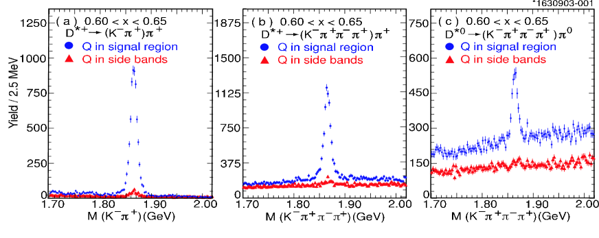
Figure 2: Examples of $M_{cand}$ distribution for two $D^{\star+}$ decay channels and one of the $D^{\star 0}$ channels analyzed. (a) $D^{\star+}$$\rightarrow$($K^{-}$$\pi^{+}$)$\pi^{+}$. (b) $D^{\star+}$$\rightarrow$($K^{-}$$\pi^{+}$$\pi^{+}$$\pi^{-}$)$\pi^{+}$. (c) $D^{\star 0}$$\rightarrow$($K^{-}$$\pi^{+}$$\pi^{+}$$\pi^{-}$)$\pi^{0}$. They show the $M_{cand}$ distribution for $Q$ in the $D^{\star+}$ signal region and for $Q$ in the $D^{\star+}$ side bands.

The choice of the signal shape used to fit the $M_{cand}$ distribution was studied and discussed in detail in a previous paper cleo1997 . A Gaussian function does not give a sufficiently accurate parametrization of the $D$ signal. Track measurement errors vary because of the geometrical orientation of the $D$ decay products in the detector, because of different momenta of the decay tracks and overlap with other tracks. That study concluded that a satisfactory choice for the $D$ signal shape is a double Gaussian, i.e., the sum of two Gaussians constrained to have the same mean. A different choice of signal fitting function is the signal shape obtained from the Monte Carlo simulation where, for each track, we can identify the input particle that generated it. We call the signal mass histograms thus obtained (one for each momentum bin) the “TAGMC shape”. To compare these two choices we repeat a test that was performed in the previous paper cleo1997 , on the $D^{0}$$\rightarrow$$K^{-}$$\pi^{+}$ channel, as follows.

We repeat the $D^{0}$ data analysis, replacing the double Gaussian with the TAGMC shape. With this signal shape we obtain excellent fits, although not superior to the double Gaussian fits. We use MINUIT to find the compatibility of the two spectra. We fit one using the other as fitting function. The fitted relative normalization parameter is $1.016\pm 0.007$, and the CL of the fit is 93.8%. The two spectra are compared in Fig. 3(a) after normalizing one to the other. To find if there is any $x_{p}$ dependence of the difference between the spectra obtained by the two methods, we took the bin-by-bin fractional difference between the two spectra (Fig. 3(b)) and fitted it to a constant, resulting into a CL=91.0%, consistent with no difference between the two choices of signal shape. The results obtained using the double Gaussian as signal shape, are compared with the TAGMC shape to estimate the systematic error on the total cross sections due to the uncertainty on the signal shape.

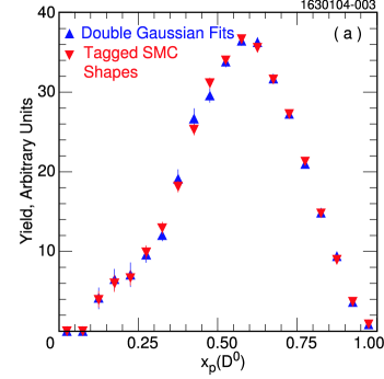
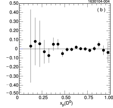
Figure 3: (a) Overlay of $D^{0}$ spectra (data) from double Gaussian and TAGMC shape signal fitting; (b) fractional difference of the two spectra.

The suitability of the double Gaussian as fitting function is also confirmed by the goodness of the fits: in all the channels, the fit confidence levels are evenly distributed between 0.0 and 1.0, as they should be. A quadratic polynomial is used to fit the combinatoric background in each of the seven channels.

The fits of the $M_{cand}$ distributions are over the whole 1.70-2.02 GeV range shown in the figures, except for the $D^{+}\to K^{-}\pi^{+}\pi^{+}$ case, where we exclude the 1.96-2.02 GeV ($D^{*+}$) region, and for the $D^{0}\to K^{-}\pi^{+}$ case, as explained in the next subsection. The fitted area of the double Gaussian (or the result of the COUNT procedure described in Sec. IV.0.2, below) is the “raw” yield for that $x_{p}$ bin.

In the next two subsections, we discuss additional backgrounds in the $M_{cand}$ distribution from the $D^{0}\to K^{-}\pi^{+}$ channel, and describe an alternative procedure, the COUNT method, to estimate the raw yield in the $D^{0}\to K^{-}\pi^{+}\pi^{-}\pi^{+}$ channel.

IV.0.1 The $D^{0}\to K^{-}\pi^{+}$ case

In the $D^{0}\to K^{-}\pi^{+}$ case (direct or from $D^{\star}$ decay) additional backgrounds must be considered: $D^{0}$ decays to $K^{-}$$K^{+}$, $\pi^{-}$$\pi^{+}$, $K^{-}$$\rho^{+}$ and $\overline{D}^{0}$$\rightarrow$$K^{+}$$\pi^{-}$  misinterpreted as $K^{-}$$\pi^{+}$. The shapes of their $M_{cand}$ distributions are obtained from Monte Carlo simulation.

The $K^{-}$$\rho^{+}$ background is very small and contributes only to the $1.70<M({K^{-}}{\pi^{+}})<1.75$ GeV mass region. This contribution is excluded by not considering this mass region in the fit.

The background due to $K$$\pi$ switched identities shows as a very broad enhancement centered at the signal position. For $x_{p}>0.20$, this enhancement is so broad that it can be easily accommodated by the quadratic term of the polynomial background function. For small $x_{p}$, it is narrower, but contributes negligibly. The amount of this background is fixed to a momentum dependent fraction determined by Monte Carlo simulation.

The backgrounds due to $D^{0}$ decays to $K^{-}$$K^{+}$, $\pi^{-}$$\pi^{+}$ do not contribute to the peak, but, if ignored, would result in a very poor fit of the background. Such a fit overestimates the amount of background under the signal and thus underestimates the amount of signal. The $D^{0}$$\rightarrow$$K^{-}$$K^{+}$ background level is a parameter to be fitted. Because of lack of statistics, the amount of $D^{0}$$\rightarrow$$\pi^{-}$$\pi^{+}$ background is constrained to a fixed fraction (0.357) of the $D^{0}$$\rightarrow$$K^{-}$$K^{+}$ background, based on the known relative branching ratio PDG . The $\pi\pi$ contribution is very small, and alternative methods of accounting for it cause negligible changes in signal yields.

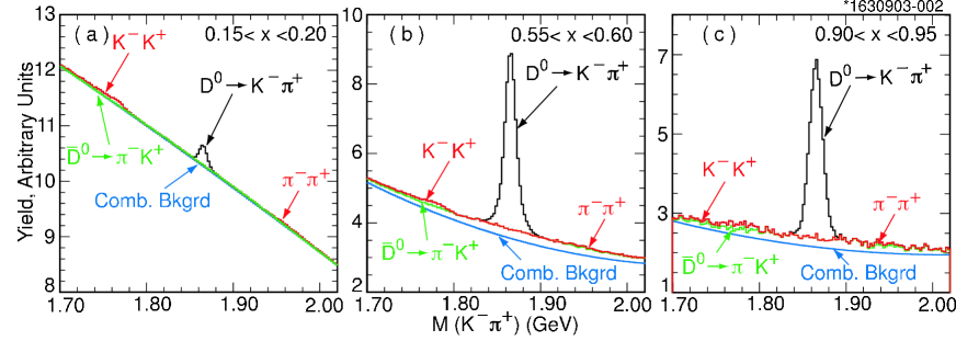
Figure 4: Buildup of the background from its components to fit the $M({K^{-}}{\pi^{+}})$ distribution. The solid histogram is data. Notice the offset on the yield axis.

Fig. 4 shows data in three representative momentum intervals, demonstrating how the background is built up from the four contributions. All four background components are needed to extract the yield.

IV.0.2 The $D^{0}\to K^{-}\pi^{+}\pi^{+}\pi^{-}$ case: the COUNT method

In the case of the $D^{0}\to K^{-}\pi^{+}\pi^{+}\pi^{-}$ decay, direct or from $D^{\star}$ decay, in addition to using a double Gaussian as fitting function for the signal, we use a different procedure that leads to results that are statistically competitive. In the $D^{0}\to K^{-}\pi^{+}\pi^{+}\pi^{-}$ case, the signal is quite narrow and the background is smooth over a wide $M_{cand}$ region. We exclude the signal region and fit the background to a polynomial. The signal region is centered on the mean of the double Gaussian fit and its range is chosen so as to contain the entire signal. We then count all events in the signal region and subtract the background obtained from this fit. The result of this subtraction is the measured signal yield. We perform this procedure on data for three choices of the signal region: 1.810-1.920 GeV, 1.820-1.910 GeV and 1.830-1.900 GeV.

We repeat this procedure on the generic Monte Carlo, thus performing the generic Monte Carlo check, described in Sec. III. The 1.820-1.910 GeV exclusion gives the best CL: 28%. The narrower exclusion gives the worst CL: 6%. The wider exclusion gives an acceptable CL: 22%, in part, because the wider the exclusion region is, the larger the statistical error becomes. Based on these results, we choose the data spectrum obtained with the 1.820-1.910 GeV exclusion as our result. The bin-by-bin rms spread of the three data spectra obtained with different signal region exclusions is taken as the estimate of the systematic error of this procedure.

We have two valid measurements, one from the COUNT method and the other from double Gaussian fitting of the signal, both performed on the same statistical sample. Hence we take as result the bin-by-bin arithmetic average of the spectrum obtained by double Gaussian fitting and the one obtained by the COUNT method with the optimal choice of the signal region exclusion: $1.820<{M_{cand}}<1.910$ GeV.

IV.1 Fit parameter smoothing

The shape parameters of the signal and background functions are expected to depend smoothly on $x_{p}$. By imposing this smoothness of the shape parameters we suppress, in part, the bin-to-bin (in $x_{p}$) statistical fluctuations in the spectra. This improves the accuracy of the shape of the spectra, particularly at low $x_{p}$ where statistics are poor. This parameter smoothing procedure was used also in our measurement of charm meson momentum spectra from $B$ decay cleo1997 . In the last paragraph of this subsection we show the extent of improvement obtained.

The parameters considered are: the mean of the double Gaussian (common to the two Gaussians), the width of the narrower Gaussian, $\sigma_{1}$, the ratio of the widths of the wider to the narrower Gaussian, $\sigma_{2}/\sigma_{1}$, and the ratio of the area of the wider Gaussian to the total area, $A_{2}/A_{tot}$. We impose this smooth behavior by fitting the $x_{p}$ dependence of each shape parameter to a polynomial, at most quadratic, in $x_{p}$.

We proceed in stages. We start by smoothing the parameter that shows the least fluctuations and repeat the $M_{cand}$ distribution fitting for all the $x_{p}$ bins, fixing that parameter to the value given by the smoothing function. We do this in sequence for all shape parameters. If a parameter does not show appreciable statistical fluctuations, we may skip smoothing it. It may take up to five iterations to smooth all the parameters.

At each stage we get a new $x_{p}$ spectrum and check that we have not introduced any distortion to that spectrum. The check is performed by calculating the bin-by-bin ratio of the new spectrum to the original one where all the parameters were allowed to float (the “no smoothing” spectrum). This ratio should show only random fluctuations around unity. If the ratio shows any trend vs $x_{p}$, e.g., if a slope and/or a curvature is needed to describe the $x_{p}$ dependence of the ratio, that smoothing stage is discarded. Fig. 5 shows three examples of these checks. When we perform a $\chi^{2}$ fit of the ratios to a constant function (=1), we obtain CL of 94.6%, 91.0% and 38.0% respectively for the three examples shown. These are typical for all the retained smoothing steps.

Figure 5: Ratios of data spectrum after double Gaussian shape parameter smoothing to the one obtained without smoothing: (a) $D^{+}$$\rightarrow$$K^{-}$$\pi^{+}$$\pi^{+}$, (b) $D^{0}$$\rightarrow$$K^{-}$$\pi^{+}$, (c) $D^{\star+}$$\rightarrow$($K^{-}$$\pi^{+}$)$\pi^{+}$.

We perform the smoothing procedure varying the sequence of smoothing stages. Each change of sequence leads to a spectrum that is slightly different from the other ones. If the CL of the generic Monte Carlo check for one of the sequences is considerably higher than the CL for the other ones, we take that spectrum as our result.

Comparison of spectra derived from different smoothing sequences provides a measure of the associated systematic error, as explained in Sec. VI.3.

We use the generic Monte Carlo check discussed in Sec. III to see if the smoothing procedure improves the agreement between the reconstructed and the original spectrum, i.e., the spectrum that is the input to the Monte Carlo simulation. In the $D^{0}$$\rightarrow$$K^{-}$$\pi^{+}$ case, when there is no smoothing, the spectrum produced by the analysis fits the original (”true”) spectrum with a $\chi^{2}=25.1$ for 15 d.o.f., i.e., CL = 5%. When smoothing is used, the spectrum produced by the analysis fits the original spectrum with $\chi^{2}=7.0$ for 15 d.o.f., i.e., CL = 95%. Thus, in this case, parameter smoothing produces a dramatic improvement. In the case of $D^{+}$$\rightarrow$$K^{-}$$\pi^{+}$$\pi^{+}$, the CL improves appreciably from 7% to 13%. In the $D^{\star+}$$\rightarrow$($K^{-}$$\pi^{+}$)$\pi^{+}$ case, where the CL is already 93% without parameter smoothing, there is only a small improvement to a CL=97%. In the $D^{\star 0}$$\rightarrow$($K^{-}$$\pi^{+}$)$\pi^{0}$ case the improvement is from CL=59% to CL=75%. As expected, the improvement is strong when the initial set of parameters show large fluctuations, smaller when the parameters show a fairly smooth behavior to start with.

V Detection Efficiency

For each channel we have two independent and statistically-compatible estimates of the detection efficiency, as explained in Sec. III. We take their weighted average, thus appreciably reducing the statistical error on the detection efficiency.

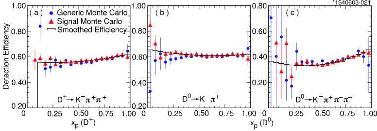
Figure 23: Direct comparison of the detection efficiencies from signal and generic Monte Carlo and the result of smoothing their average: (a) for the $D^{+}$$\rightarrow$$K^{-}$$\pi^{+}$$\pi^{+}$ channel, (b) for the $D^{0}$$\rightarrow$$K^{-}$$\pi^{+}$ channel, and (c) for the $D^{0}$$\rightarrow$$K^{-}$$\pi^{+}$$\pi^{+}$$\pi^{-}$ channel.

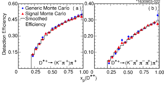
Figure 24: Comparison of the detection efficiencies obtained from the signal and generic Monte Carlo and their smoothed average: (a) for the $D^{*+}\rightarrow D^{0}\pi^{+}\rightarrow(K^{-}\pi^{+})\pi^{+}$ channel, (b) for the $D^{*+}\rightarrow D^{0}\pi^{+}\rightarrow(K^{-}\pi^{+}\pi^{-}\pi^{+})\pi^{+}$ channel.

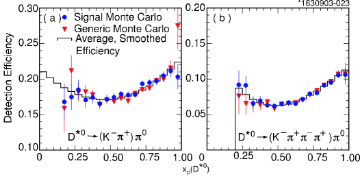
Figure 25: Comparison of the unsmoothed detection efficiencies obtained from the signal and generic Monte Carlo: (a) for the $D^{*0}\rightarrow D^{0}\pi^{0}\rightarrow(K^{-}\pi^{+})\pi^{0}$, (b) for the $D^{*0}\rightarrow D^{0}\pi^{0}\rightarrow(K^{-}\pi^{+}\pi^{-}\pi^{+})\pi^{0}$ channel.

The detection efficiency should be a smooth function of $x_{p}$. We use a second order polynomial to fit the $x_{p}$ dependence of the detection efficiency averaged over the signal and generic Monte Carlo. Adding a cubic term does not improve any of the fits. We call the result of this fit the “smoothed efficiency”. In Appendix A, we show the detection efficiency dependence on $x_{p}$ for all the mesons and decay modes analyzed. In Figs. 23, 24, 25, the detection efficiencies obtained from the signal and generic Monte Carlo’s are plotted, and the curve resulting from the fit of their average to a polynomial is overlaid. This procedure results in a strong reduction of the statistical errors on the detection efficiency.

The detection efficiency corrected spectrum is obtained by dividing the raw signal yield by the smoothed efficiency, bin-by-bin in $x_{p}$.

VI Checks and error estimation

VI.1 Two Checks

VI.1.1 Generic Monte Carlo checks

For each procedure used to reconstruct the spectra, we perform a “generic Monte Carlo check”, as described in Sec. III. The confidence levels reported below in Table 1, show the consistency of the reconstructed spectrum with the original one. Since our interest is in the consistency of the shapes of the two spectra, we do the comparison after normalizing the areas of the the two spectra to each other. The normalization differs from unity by at most 2.6%. Notice that in the generic Monte Carlo checks we can only use the signal Monte Carlo efficiency, not the averaged, smoothed efficiency described in the previous section (Sec. V).

Table 1: Confidence levels of the fit of the generic Monte Carlo reconstructed spectrum to its input spectrum for the seven decay channels analyzed.

Decay channel	C.L.	Decay channel	C.L.	Decay channel	C.L.
$D^{+}\rightarrow K^{-}\pi^{+}\pi^{+}$	18%	$D^{0}\rightarrow K^{-}\pi^{+}$	72%	$D^{0}\rightarrow K^{-}\pi^{+}\pi^{+}\pi^{-}$	56%
$D^{*+}\rightarrow(K^{-}\pi^{+})\pi^{+}$	70%	$D^{*+}\rightarrow(K^{-}\pi^{+}\pi^{+}\pi^{-})\pi^{+}$	37%	$D^{*0}\rightarrow(K^{-}\pi^{+})\pi^{0}$	76%
		$D^{*0}\rightarrow(K^{-}\pi^{+}\pi^{+}\pi^{-})\pi^{0}$	99%

VI.1.2 Comparison of spectra from different decay modes

In the $D^{0}$, $D^{\star+}$ and $D^{\star 0}$ cases we obtain the respective spectra from two different $D^{0}$ decay modes. We checked that the spectra from the two different decay modes are statistically compatible. We calculate the $\chi^{2}$ of the difference, using only the statistical errors. The corresponding confidence levels are, respectively, 28%, 100% and 0.09%. After normalizing one to the other the confidence level become: 85%, 100% and 84%. This test, however, is not very stringent because the comparison is dominated by the large statistical errors of the $D^{0}\to K^{-}\pi^{+}\pi^{+}\pi^{-}$ channel.

VI.2 Statistical Errors

The statistical errors on the efficiency-corrected yields are obtained by adding in quadrature the statistical error on the raw yield and the statistical error on the smoothed efficiency (Sec. V). The latter is generally considerably smaller than the former.

VI.3 Systematic Errors

We discuss here systematic errors that could affect the shape of the differential cross section $d\sigma/dx_{p}$, although some of them are found to be independent of $x_{p}$. Additional systematic errors that affect the normalization of the differential cross section, but not its shape, will be discussed in Sec. VIII on total cross sections.

VI.3.1 Errors found to be independent of $x_{p}$ or negligible.

We consider the following possible sources of systematic errors: (1) the choice of signal fitting function, (2) possibly incorrect simulation of the initial state radiation, (3) effects of swapping between background curvature and width of the wide Gaussian in $M_{cand}$ distribution fitting, and (4) effects of low detection efficiency for very low momentum tracks.

The test, described in Sec. IV, that uses a signal fitting function other than a double Gaussian, gives us a measure of the sensitivity of our results to the choice of signal fitting function. Based on that test, we attribute a systematic error of 1.6% from the choice of signal fitting function. The test shows no momentum dependence of the difference between the two methods.

We have considered the possibility that inaccurate simulation of initial state radiation (ISR) may have introduced a systematic error in our estimate of the detection efficiencies. We compare the detection efficiencies discussed in Sec. V with those obtained from Monte Carlo events where no ISR was produced. As expected, the latter is slightly higher than the former, but only by 1.1%, and its dependence on $x_{p}$ is negligible. Since our Monte Carlo does simulate the initial state radiation, the uncertainty is only in the accuracy of the simulation. We thus take half of that, 0.5%, as contribution to the systematic error on the cross sections.

Since the momentum dependence of these two uncertainties is found to be negligible, we take them into account only as errors in the total cross sections (Sec. VIII).

We considered the possibility of swapping between a background that is highly curved in the signal region, and the wide component of the double Gaussian. The only two channels that show an appreciable background curvature are $D^{0}$$\rightarrow$$K^{-}$$\pi^{+}$$\pi^{+}$$\pi^{-}$and $D^{+}$$\rightarrow$$K^{-}$$\pi^{+}$$\pi^{+}$. In the first case the full compatibility of the fits with the results of the COUNT procedure (subsect. IV.0.2, CL$>96$% for both Monte Carlo’s and for data), shows that this swapping, if it exists, generates an error much smaller than the statistical error. In the $D^{+}$ case we performed the same test with the same result.

We considered the possibility of errors in the $D^{\star+}$ detection efficiency because of the very rapid decrease in the charged track detection efficiency for momenta below 120 MeV/c. The detection efficiency is practically zero below 70 MeV/c. We studied in detail the momentum distribution of the charged $\pi^{\pm}$ daughter of the $D^{\star\pm}$ (the “slow pion”) as a function of $x_{p}$($D^{\star\pm}$). Only for $x_{p}({D^{\star\pm}})<0.40$ are there slow pions with momentum below 120 MeV/c. From the momentum dependence of the track detection efficiency and the $D^{\star\pm}$ isotropic decay distribution D*align , we can calculate the $D^{\star\pm}$ detection efficiency. The result is consistent with the one resulting from our generic and signal Monte Carlo simulation within their statistical errors.

Since we find the errors from these last two sources to be negligible, we disregard them.

VI.3.2 Errors that affect the spectra shapes

The different sequences of parameter smoothing stages (described in Sec. IV.1) lead to slightly different resulting spectra. We calculate the root-mean-square (rms) spreads of the yields for each $x_{p}$ bin over the spectra from different sequences. Since these rms spreads fluctuate statistically from bin to bin, as expected, we average them over groups of three bins. We take these rms spreads as systematic errors on the yields.

As stated in Sec. III, we have both generic and signal Monte Carlo samples of events, and to the extent that our Monte Carlo correctly simulates data and detector, we can perform a test which give comprehensive information on all systematic errors associated with our analysis procedures. We take the bin-by-bin difference between the generic Monte Carlo reconstructed spectrum and the input spectrum, and divide this, bin-by-bin, by the input spectrum, resulting in the distribution of the fractional difference vs $x_{p}$. The weighted average, over the entire $x_{p}$ range, of the absolute values of these fractional differences (where the weights are the inverse square errors on the differences) can be considered as an estimate of the systematic error. It varies from 0.6% for the $D^{0}$$\rightarrow$$K^{-}$$\pi^{+}$ channel to 1.4% for the $D^{+}$$\rightarrow$$K^{-}$$\pi^{+}$$\pi^{+}$ channel. The distributions of the fractional differences show negligible dependence on $x_{p}$, meaning that this estimated systematic error does not seem to affect the shape of the spectra. Nevertheless we include these average differences as a component of the systematic error on the measured yields. In principle, this estimate of the systematic error takes into account also the “rms spreads” discussed in the previous paragraph. We decided, however, to be conservative, and have combined them in quadrature to obtain the total systematic error. Even with possible overestimate, generally the systematic error makes the total error larger than the statistical error by only 10% to 30%.

VI.4 Total errors

The statistical errors and the two systematic errors affecting the spectra shapes are listed, channel by channel, in Table 5 - 11 in Appendix B. These three errors are combined in quadrature to give total errors relevant to the shape of our spectra.

VII Results on the shape of the Spectra

VII.1 The Final or Combined Spectrum.

For each $D$ or $D^{\star}$ meson and its decay chain, we obtain the spectrum fitting the signal with a double Gaussian after smoothing the $x_{p}$ dependence of the Gaussian parameters, as described in Sec. IV.1. When we also employ the COUNT method, as explained in Sec. IV.0.2, the spectrum that we report is the average of the spectrum obtained by fitting a double Gaussian and that obtained with the COUNT method. Details specific to each channel, are given in the sections showing the respective spectra.

The spectra shown in the following are differential, inclusive production cross sections, $d\sigma({e^{+}e^{-}}\to D^{(*)}X)/dx_{p}$ at $\sqrt{s}=10.58$ GeV fully corrected for detection efficiency and decay branching ratios. We use the following decay branching ratios: $\cal B$($D^{0}$$\rightarrow$$K^{-}$$\pi^{+}$)=(3.82$\pm$0.09)%, $\cal B$($D^{0}$$\rightarrow$$K^{-}$$\pi^{+}$$\pi^{-}$$\pi^{+}$)=(7.49$\pm$0.31)%, $\cal B$($D^{+}$$\rightarrow$$K^{-}$$\pi^{+}$$\pi^{+}$)=(9.0$\pm$0.6)%, $\cal B$($D^{\star+}$$\rightarrow$$D^{0}$$\pi^{+}$)=(67.6$\pm$0.5)%, $\cal B$($D^{\star 0}$$\rightarrow$$D^{0}$$\pi^{0}$)=(61.9$\pm$2.9)%. They affect only the normalization, not the shape, of the spectra. Uncertainties in the branching ratios will be reflected in the systematic errors on the total cross sections, Sec. VIII.

VII.2 $D^{+}$ Spectrum

Fig. 6 shows examples of fits to the $M_{cand}$ distributions in three representative $x_{p}$ bins, using fully smoothed parameters. Our result is shown in Fig. 7 and tabulated in App. B, Table 5. The spectrum shown is obtained after smoothing the $x_{p}$ dependence of the double Gaussian shape parameters (see Sec. IV.1) using the sequence that gives the best CL in the generic Monte Carlo check (Sec. VI.1).

Figure 6: Three examples of $M({K^{-}}{\pi^{+}}{\pi^{+}})$ distribution fits. Notice the large vertical scale offsets.

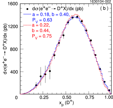
Figure 7: Differential cross section $d\sigma(e^{+}e^{-}\to D^{+}X)/dx_{p}$ in pb from the $D^{+}$$\rightarrow$$K^{-}$$\pi^{+}$$\pi^{+}$ decay mode. (a) shows explicitly the total and statistical errors. (b) the same spectrum overlaid with the JETSET spectra generated with two different sets of parameters (Sec. IX).

VII.3 $D^{0}$ Spectrum

VII.3.1 $D^{0}$Spectrum from $D^{0}$$\rightarrow$$K^{-}$$\pi^{+}$

Fig. 8 shows examples of fits to the $M_{cand}$ distributions in three representative $x_{p}$ bins, using fully smoothed parameters.

Figure 8: Three examples of $M({K^{-}}{\pi^{+}})$ distribution fits. Notice the large y offsets.

The $D^{0}$ inclusive, differential production cross section obtained from this decay mode is shown in Fig. 9 and in App. B, Table 6. It is obtained after smoothing the $x_{p}$ dependence of the double Gaussian shape parameters (see Sec. IV.1) using the sequence that gives the best CL in the generic Monte Carlo check (Sec. VI.1).

Figure 9: Differential cross section $d\sigma(e^{+}e^{-}\to D^{0}X)/dx_{p}$ in pb from the $D^{0}\rightarrow K^{-}\pi^{+}$ decay mode.

VII.3.2 $D^{0}$ Spectrum from $D^{0}$$\rightarrow$$K^{-}$$\pi^{+}$$\pi^{+}$$\pi^{-}$

Fig. 10 shows examples of fits to the $M_{cand}$ distributions in three representative $x_{p}$ bins, with no parameter smoothing. Because of the large statistical errors, we find the Gaussian parameter smoothing procedure to be unreliable. However, as discussed in Sec. IV.0.2, for this mode we use also the COUNT method with three different widths of the excluded signal region in order to get part of the systematic error on this procedure.

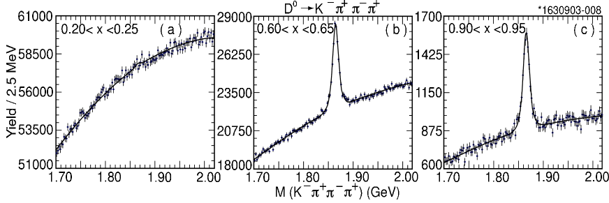
Figure 10: Three examples of $M({K^{-}}{\pi^{+}}{\pi^{+}}{\pi^{-}})$ distribution fits. Notice the large y offsets.

Figure 11: Differential cross section $d\sigma(e^{+}e^{-}\to D^{0}X)/dx_{p}$ in pb from the $D^{0}\rightarrow K^{-}\pi^{+}\pi^{+}\pi^{-}$ decay mode.

The $D^{0}$ inclusive, differential production cross section obtained from this decay mode is shown in Fig. 11 and tabulated in App. B, Table 7. It is the arithmetic average of the one obtained by double Gaussian fits (without any Gaussian parameter smoothing) and the one produced with the COUNT procedure, excluding from the background fit the 1.820-1.910 GeV region. For the final statistical errors we take the average of the statistical errors associated with the two methods.

VII.3.3 The Average $D^{0}$ Spectrum

The weighted average of the spectra obtained from the two $D^{0}$ decay modes analyzed is shown in Fig. 12 and tabulated in App. B, Table 12. The two JETSET generated spectra are explained in Sec. IX.

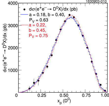
Figure 12: Differential cross section $d\sigma(e^{+}e^{-}\to D^{0}X)/dx_{p}$, weighted average of the spectra from the $D^{0}$$\rightarrow$$K^{-}$$\pi^{+}$ and $D^{0}$$\rightarrow$$K^{-}$$\pi^{+}$$\pi^{+}$$\pi^{-}$ decay modes, overlaid with the JETSET spectra generated with two different sets of parameters (Sec. IX).

VII.4 The $D^{\star+}$ Spectrum

In Sec. IV we described our procedure for selecting $D^{\star+}$ candidates. The difference between the two $M_{cand}$ distributions shown in Fig. 2 eliminates random $D^{0}$$\pi^{+}$ associations.

VII.4.1 $D^{\star+}$ Spectrum from $D^{\star+}$$\rightarrow$$D^{0}$$\pi^{+}$$\rightarrow$($K^{-}$$\pi^{+}$)$\pi^{+}$

The subtracted $M_{cand}$ distribution (Fig. 13) shows the additional backgrounds present in this $D^{0}$ decay mode. They have been handled as described in Sec. IV.0.1.

Figure 13: Three examples of fits of the subtracted $M({K^{-}}{\pi^{+}})$ distributions for $D^{*+}\rightarrow D^{0}\pi^{+}\rightarrow(K^{-}\pi^{+})\pi^{+}$ candidates.

The spectrum is shown in Fig. 14 and tabulated in App. B, Table 8. It is the one obtained after smoothing the $x_{p}$ dependence of the double Gaussian shape parameters (see Sec. IV.1) using the sequence that gave the best CL in the generic MC check (Sec. VI.1).

Figure 14: $d\sigma({e^{+}e^{-}}\rightarrow D^{*+}X)/dx_{p}$, from the $D^{*+}\rightarrow D^{0}\pi^{+}\rightarrow(K^{-}\pi^{+})\pi^{+}$ decay mode.

VII.4.2 $D^{\star+}$ Spectrum from $D^{\star+}$$\rightarrow$$D^{0}$$\pi^{+}$$\rightarrow$($K^{-}$$\pi^{+}$$\pi^{+}$$\pi^{-}$)$\pi^{+}$

Just as in the case of $D^{0}\rightarrow K^{-}\pi^{+}\pi^{+}\pi^{-}$, taking advantage of the narrowness of the signal over a background that is smooth and well determined over a large region, we use the COUNT procedure described in Sec. IV.0.2 with the signal region exclusion as optimized in that analysis (1.820-1.910 GeV). The $Q$ selection reduces drastically the background with respect the $D^{0}$ case, and we obtain good double Gaussian fits of the signal as shown, for three representative $x_{p}$ bins, in Fig. 15.

Figure 15: Three examples of fits of the subtracted $M({K^{-}}{\pi^{+}}{\pi^{-}}{\pi^{+}})$ distributions for $D^{*+}\rightarrow D^{0}\pi^{+}\rightarrow(K^{-}\pi^{+}\pi^{-}\pi^{+})\pi^{+}$ candidates.

Figure 16: $d\sigma({e^{+}e^{-}}\rightarrow D^{*+}X)/dx_{p}$ from the $D^{*+}\rightarrow D^{0}\pi^{+}\rightarrow(K^{-}\pi^{+}\pi^{-}\pi^{+})\pi^{+}$ decay mode.

The spectrum is shown in Fig. 16 and tabulated in App. B, Table 9. It is the arithmetic average of the one obtained by double Gaussian fit, after full smoothing of the $x_{p}$ dependence of the double Gaussian shape parameters (see Sec. IV.1), and the one produced with the COUNT procedure, excluding from the background fit the 1.820-1.910 GeV region.

VII.4.3 The Average $D^{\star+}$ Spectrum

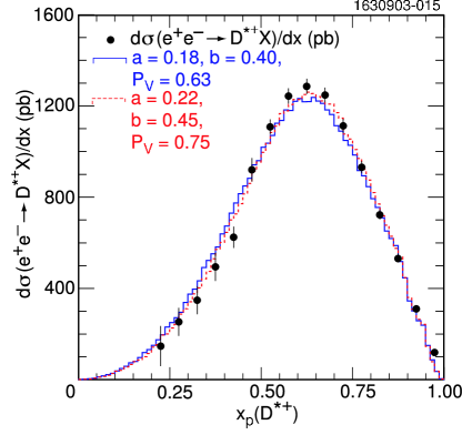
Figure 17: Differential cross section $d\sigma(e^{+}e^{-}\to D^{*+}X)/dx_{p}$, weighted average of $D^{\star+}$$\rightarrow$$D^{0}$$\pi^{+}$$\rightarrow$($K^{-}$$\pi^{+}$)$\pi^{+}$and $D^{\star+}$$\rightarrow$$D^{0}$$\pi^{+}$$\rightarrow$($K^{-}$$\pi^{+}$$\pi^{+}$$\pi^{-}$)$\pi^{+}$spectra, overlaid with the JETSET spectra generated with two sets of parameters (Sec. IX).

The weighted average of the spectra obtained from the two decay modes analyzed is shown in Fig. 17 and tabulated in App. B, Table 12. The two JETSET generated spectra are explained in Sec. IX.

VII.5 $D^{\star 0}$ Spectrum

To suppress random $D^{0}$$\pi^{0}$ associations, we use the subtraction procedure already used for the $D^{\star+}$ cases and illustrated in Fig. 2.

VII.5.1 $D^{\star 0}$ Spectrum from $D^{\star 0}$$\rightarrow$$D^{0}$$\pi^{0}$$\rightarrow$($K^{-}$$\pi^{+}$)$\pi^{0}$

Figure 18: Three examples of fits of the $M({K^{-}}{\pi^{+}})$ distributions for $D^{*0}\rightarrow D^{0}\pi^{0}\rightarrow(K^{-}\pi^{+})\pi^{0}$ candidates.

Fig. 18 shows three examples of fits of the subtracted $M_{cand}$ distribution for this channel. Here too we add to the fitting functions the backgrounds described in Sec. IV.0.1.

The differential cross section is shown in Fig. 19 and tabulated in in App. B, Table 10. Among the different stage sequences in smoothing the Gaussian parameters (see Sec. IV.1) we choose the one that gives the best CL in the generic MC check (Sec. VI.1).

Figure 19: $d\sigma({e^{+}e^{-}}\rightarrow D^{*0}X)/dx_{p}$, from the $D^{*0}\rightarrow D^{0}\pi^{0}\rightarrow(K^{-}\pi^{+})\pi^{0}$ decay mode.

VII.5.2 $D^{\star 0}$ Spectrum from $D^{\star 0}$$\rightarrow$$D^{0}$$\pi^{0}$$\rightarrow$($K^{-}$$\pi^{+}$$\pi^{+}$$\pi^{-}$)$\pi^{0}$

Fig. 20 shows, for three representative $x_{p}$ bins, the fits of the subtracted $M_{cand}$ distribution, using a double Gaussian and a polynomial background.

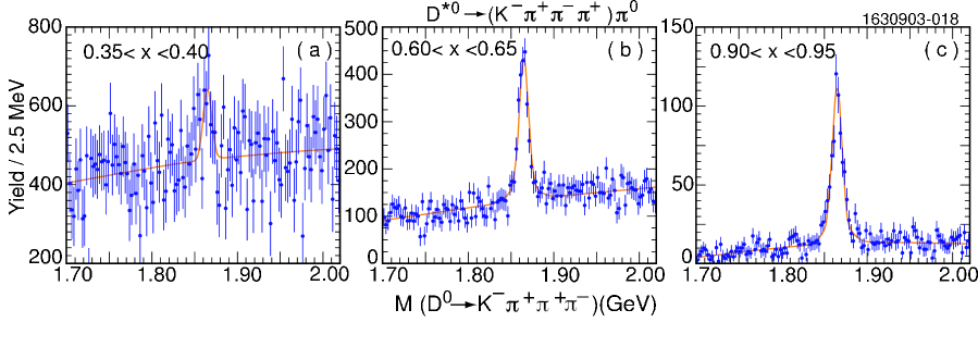
Figure 20: Three examples of fits of the subtracted $M({K^{-}}{\pi^{+}}{\pi^{-}}{\pi^{+}})$ distributions for $D^{*0}\rightarrow D^{0}\pi^{0}\rightarrow(K^{-}\pi^{+}\pi^{-}\pi^{+})\pi^{0}$ candidates.

Because of the smaller decay branching ratio and the smaller detection efficiency, due to the presence of a $\pi^{0}$, the statistical errors are quite large, especially for ${x_{p}}<0.50$, where we can use only the continuum events. We have used both the COUNT procedure and the double Gaussian signal fitting (without parameter smoothing) to get the $D^{\star 0}$ yield.

Figure 21: $d\sigma({e^{+}e^{-}}\rightarrow D^{*0}X)/dx_{p}$, from the $D^{*0}\rightarrow D^{0}\pi^{0}\rightarrow(K^{-}\pi^{+}\pi^{-}\pi^{+})\pi^{0}$ decay mode.

The spectrum is shown in Fig. 21 and tabulated in App. B, Table 11. It is the arithmetic average of that obtained by fitting the signal with the double Gaussian (smoothed parameters) and the one obtained by the COUNT method using the signal region exclusion optimized in that analysis (1.820-1.910 GeV).

VII.5.3 The Average $D^{\star 0}$ Spectrum

The weighted average of the spectra obtained from the two decay modes analyzed is shown in Fig. 22 and listed in App. B, Table 12. The two JETSET generated spectra are explained in Sec. IX.

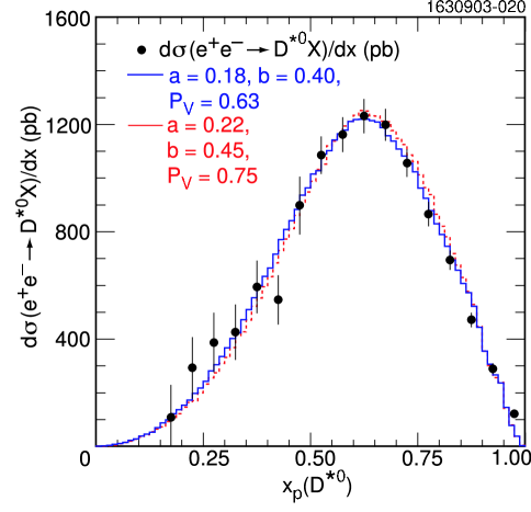
Figure 22: $d\sigma(e^{+}e^{-}\to D^{*0}X)/dx_{p}$, weighted average of the $D^{\star 0}$$\rightarrow$$D^{0}$$\pi^{0}$$\rightarrow$($K^{-}$$\pi^{+}$)$\pi^{0}$ and $D^{\star 0}$$\rightarrow$$D^{0}$$\pi^{0}$$\rightarrow$($K^{-}$$\pi^{+}$$\pi^{+}$$\pi^{-}$)$\pi^{0}$decay modes. Overlaid are the JETSET spectra generated with two sets of parameters (Sec. IX).

VIII Results for the Total Cross Sections and average $x_{p}$

The production cross section for each channel is shown in Table 3. It is calculated by summing each differential cross section bin-by-bin. The first error in the table is the statistical error, obtained by combining in quadrature the statistical errors in each bin. If the yield in the lowest few bins cannot be reliably measured, the cross section is corrected by extrapolating the spectrum to $x_{p}=0$ using the JETSET distribution that fits the spectrum, discussed in Sec. IX. This correction is between 0.2% and 6%.

In Table 2 we list, channel by channel, the components of the systematic error on the production cross sections. In the first column we report the rms spread of the cross sections obtained by the four or five smoothing sequences used for each channel. The discrepancy between the areas of the input and reconstructed spectra in the generic Monte Carlo check (Sec. VI.1), is shown in the second column. In the third column we list the percent difference between the integral of the spectra obtained using the double Gaussian and the one that uses the TAGMC signal shape (Sec. IV). This error is not considered for the channels where the $D^{0}$ decays to $K^{-}$$\pi^{+}$$\pi^{+}$$\pi^{-}$, because of the use of the COUNT procedure for those channels. We assume a 10% error on the extrapolation and show it in column 4. The remaining systematic errors are estimated and discussed in a series of CLEO internal notes and are used in all CLEO analyses where they are relevant. We estimate a 1% per track uncertainty in the charged-track detection efficiency and 0.8% per track for particle identification efficiency. The choice of track quality and geometrical cuts result in an error of 0.5% also per track. The per track errors, being coherent, are multiplied by the number of tracks in the decay, and are shown in columns 5, 6, and 7. The $\pi^{0}$ detection uncertainty is estimated to be 3% per $\pi^{0}$ (column 8). As discussed in Sec. VI.3, we attribute a 0.5% error due to possible inaccuracies in the Monte Carlo simulation of the initial state radiation. The error on the integrated luminosity is estimated as 1.9%.

Table 2: Systematic errors described in the text. Some are listed as percent of the cross section, other ones directly in pb. The momentum dependent systematic errors are listed also in the tables in App. B. The error due to the uncertainty on the branching ratio is shown only in Table 3.

	1	2	3	4	5	6	7	8	9	10
	procedures	gMC	signal	Extra-	track	part.	other	$\pi^{0}$	ISR
Decay channel	rms	check	shape	polat.	det.eff.	ID	sel.	det.	sim.	Lum.
$D^{+}\rightarrow K^{-}\pi^{+}\pi^{+}$	5pb	15pb	1.6%	0.5pb	3%	2.4%	1.5%		0.5%	1.9%
$D^{0}\rightarrow K^{-}\pi^{+}$	22pb	8pb	1.6%	0.4pb	2%	1.6%	1.0%		0.5%	1.9%
$D^{0}\rightarrow K^{-}\pi^{+}\pi^{+}\pi^{-}$	41pb	29pb		3.2pb	4%	3.2%	2.0%		0.5%	1.9%
$D^{*+}\rightarrow(K^{-}\pi^{+})\pi^{+}$	8pb	15pb	1.6%	0.9pb	3%	2.4%	1.5%		0.5%	1.9%
$D^{*+}\rightarrow(K^{-}\pi^{+}\pi^{+}\pi^{-})\pi^{+}$	17pb	7pb		3.3pb	5%	4.0%	2.5%		0.5%	1.9%
$D^{*0}\rightarrow(K^{-}\pi^{+})\pi^{0}$	11pb	10pb	1.6%	3.6pb	2%	1.6%	1.0%	3%	0.5%	1.9%
$D^{*0}\rightarrow(K^{-}\pi^{+}\pi^{+}\pi-)\pi^{0}$	45pb	12pb		1.1pb	4%	3.2%	2.0%	3%	0.5%	1.9%

These systematic errors are combined in quadrature to give the systematic error on the cross section, the second entry in Table 3.

Table 3: Total production cross sections and average $x_{p}$, as derived from each decay mode. The cross section errors are, in this order, the statistical error, the systematic error and the error due to the uncertainty on the branching ratio.

Decay channel	Total Cross Section (pb) at 10.5 GeV C.M.E.
$D^{+}\rightarrow K^{-}\pi^{+}\pi^{+}$	$\sigma({e^{+}e^{-}}\to D^{+}X)=640{\pm}14{\pm}35{\pm}43$
$D^{0}\rightarrow K^{-}\pi^{+}$	$\sigma({e^{+}e^{-}}\to D^{0}X)=1,521{\pm}16{\pm}62{\pm}36$
$D^{0}\rightarrow K^{-}\pi^{+}\pi^{+}\pi^{-}$	$\sigma({e^{+}e^{-}}\to D^{0}X)=1,579{\pm}55{\pm}102{\pm}63$
$D^{*+}\rightarrow D^{0}\pi^{+}\rightarrow(K^{-}\pi^{+})\pi^{+}$	$\sigma({e^{+}e^{-}}\to D^{*+}X)=583{\pm}8{\pm}33{\pm}14$
$D^{*+}\rightarrow D^{0}\pi^{+}\rightarrow(K^{-}\pi^{+}\pi^{+}\pi^{-})\pi^{+}$	$\sigma({e^{+}e^{-}}\to D^{*+}X)=572{\pm}26{\pm}45{\pm}24$
$D^{*0}\rightarrow D^{0}\pi^{0}\rightarrow(K^{-}\pi^{+})\pi^{0}$	$\sigma({e^{+}e^{-}}\to D^{*0}X)=559{\pm}24{\pm}35{\pm}29$
$D^{*0}\rightarrow D^{0}\pi^{0}\rightarrow(K^{-}\pi^{+}\pi^{+}\pi-)\pi^{0}$	$\sigma({e^{+}e^{-}}\to D^{*0}X)=616{\pm}32{\pm}62{\pm}39$

We calculate $<x_{p}>$ for the $D^{+}$ spectrum and for the spectra of $D^{0}$, $D^{*+}$ and $D^{*0}$ averaged over the decay modes. We supplement the data spectrum in the lowest bins using the JETSET spectra normalized to the spectra. We take the errors on these “borrowed” cross sections to be roughly comparable to the data in nearby bins. The results are shown in Table 4.

Table 4: $<x_{p}>$ for the four charm mesons considered. The first error is statistical, the second systematic.

Meson	$<x_{p}>$	Meson	$<x_{p}>$
$D^{+}$	$0.582\pm 0.008\pm 0.004$	$D^{*+}$	$0.611\pm 0.007\pm 0.004$
$D^{0}$	$0.570\pm 0.005\pm 0.004$	$D^{*0}$	$0.596\pm 0.009\pm 0.004$

IX Optimization of JETSET parameters

Largely for internal use of our collaboration, we perform a simple fit of the $D^{0}$ spectrum (from the $D^{0}$$\rightarrow$$K^{-}$$\pi^{+}$ decay mode) varying the three JETSET parameters that are most important for the shape of the spectrum. The first and second are the parameters $a$ and $b$ appearing in the “Lund Symmetric Fragmentation Function” Boand ; LundSM :

$$f(z)=N\frac{(1-z)^{a}}{z}\exp\left[\frac{-b\cdot m^{2}_{\bot}}{z}\right]$$ (3)

where $z$ is the reduced energy $x_{E}$, or momentum $x_{p}$, of the hadron and $m^{2}_{\bot}=m^{2}+p^{2}_{\bot}$, with $m$ being the hadron mass and $p_{\bot}$ the component of the hadron momentum perpendicular to the jet axis.

The third parameter is the probability $P_{V}$ that a meson of given flavor be generated as a vector meson, rather than pseudoscalar or tensor, $P_{V}\equiv V/(P+V+T)$. The data indicate, as expected, that the majority of $D^{0}$’s are not produced directly in the fragmentation of the charm quark, but from the decay of $D^{\star}$’s. In JETSET jtst74 these parameters are PARJ(41), PARJ(42) and PARJ(13).

The result of the fit of the $D^{0}$ spectrum (in the $K^{-}$$\pi^{+}$ decay mode) is:

$$a=0.178\pm 0.007,\hskip 28.90755ptb=0.393{\pm}0.006,\hskip 28.90755ptP_{V}=0.627\pm 0.015.$$

Keeping $P_{V}$ fixed at the naive value $P_{V}=0.75$, we obtain $a=0.223{\pm}0.009$ and $b=0.438{\pm}0.005$. In both cases the quoted errors are simple statistical errors. Correlation between parameters are not evaluated. The spectra resulting from these parameterizations are shown in Fig. 7,  12, 17, 22.

Notice that we do not consider our results of $D^{+}$, $D^{\star+}$ and $D^{\star 0}$ spectra in the optimization process. However, a posteriori we see, visually from the figures, that the spectra generated with these parameters seem to reproduce rather accurately also the $D^{+}$, $D^{\star+}$ and $D^{\star 0}$ experimental distributions. However, it is not obvious which one of the two sets, the one with $P_{V}=0.672$ or the one with $P_{V}=0.75$, should be preferred. Furthermore, these parameters, while useful for the Monte Carlo simulation of $D$ and $D^{\star}$ spectra at the c.m. energy of our and similar experiments, should not be taken as having general validity and theoretical significance. In fact, the $D_{s}^{+}$ spectrum generated by JETSET with our fitted parameters disagrees appreciably with the spectrum measured by the CLEO EdJohn and BaBar BabarDs collaborations. It should be noted that the effect of these parameters may also be influenced by the value of other JETSET parameters.

X Conclusions

We have measured the momentum distribution of $D^{0}$, $D^{+}$, $D^{\star+}$ and $D^{\star 0}$ produced in non-resonant $e^{+}e^{-}$ annihilation at a CME of about 10.5 GeV. These distributions can be used to guide and check QCD calculations of fragmentation functions needed to predict heavy meson production in both $e^{+}e^{-}$ annihilation and hadron collisions at very high energy. The $D^{0}$ spectrum was used to determine the JETSET parameters that best reproduce it, and we found that, with these parameters, the $D^{\star}$, $D^{\star+}$ and $D^{\star 0}$ spectra (but not the $D_{s}^{+}$ spectrum) are also well reproduced.

Appendix A Plots of detection efficiencies vs $x_{p}$

In the following figures we show the detection efficiency dependence on $x_{p}$ for all the mesons and decay modes analyzed. The detection efficiencies obtained from the signal and generic MC simulations are plotted, together with the curve resulting from the fit of their weighted average to a polynomial.

Appendix B Tables of differential cross sections

In the following tables, we report the quantity $d\sigma/dx_{p}$ in pb. Notice that the systematic and total errors are errors on the bin content (i.e., the first column). The first column of systematic errors is obtained from the rms spread of yields for the different procedures used to calculate the spectrum. The second column of systematic errors is derived from the “generic MC check” described in Sec. VI.1. These are the errors relevant to the shape of the spectra, i.e., they do not include the systematic errors that are common to the whole momentum range and that contribute to the error on the cross section (Sec. VIII).

Table 5: $d\sigma(e^{+}e^{-}\to D^{+}X)/dx_{p}$ in pb; ($D^{+}$$\rightarrow$$K^{-}$$\pi^{+}$$\pi^{+}$)

	$d\sigma/dx_{p}$	Errors (pb)
$x_{p}$	(pb)	Statistical	Systematic		Total
0.15-0.20	161	78	27	3	83
0.20-0.25	320	76	53	5	92
0.25-0.30	356	70	59	6	92
0.30-0.35	413	64	68	7	94
0.35-0.40	693	58	11	11	60
0.40-0.45	909	52	14	15	56
0.45-0.50	1042	47	16	17	53
0.50-0.55	1271	25	20	21	38
0.55-0.60	1357	22	21	22	38
0.60-0.65	1370	19	21	22	36
0.65-0.70	1291	17	20	21	34
0.70-0.75	1129	15	17	18	29
0.75-0.80	952	13	15	16	25
0.80-0.85	694	10	11	11	19
0.85-0.90	449	8	7	7	13
0.90-0.95	223	5	3	4	7
0.95-1.00	74	3	1	1	4

Table 6: $d\sigma(e^{+}e^{-}\to D^{0}X)/dx_{p}$ in pb; ($D^{0}$$\rightarrow$$K^{-}$$\pi^{+}$).

	$d\sigma/dx_{p}$	Errors (pb)
$x_{p}$	(pb)	Statistical	Systematic		Total
0.10-0.15	196	86	73	1	113
0.15-0.20	507	92	188	3	209
0.20-0.25	597	85	221	3	237
0.25-0.30	891	76	37	5	85
0.30-0.35	1154	68	48	7	84
0.35-0.40	1665	63	70	10	95
0.40-0.45	2341	61	98	13	116
0.45-0.50	2889	59	121	17	136
0.50-0.55	3178	35	42	18	57
0.55-0.60	3444	34	45	20	60
0.60-0.65	3345	34	44	19	58
0.65-0.70	2984	33	39	17	54
0.70-0.75	2542	31	33	15	48
0.75-0.80	1997	29	26	11	41
0.80-0.85	1380	25	18	8	32
0.85-0.90	831	19	11	5	23
0.90-0.95	337	11	4	2	12
0.95-1.00	78	5	1	0.4	6

Table 7: $d\sigma(e^{+}e^{-}\to D^{0}X)/dx_{p}$ in pb; ($D^{0}$$\rightarrow$$K^{-}$$\pi^{+}$$\pi^{+}$$\pi^{-}$).

	$d\sigma/dx_{p}$	Errors (pb)
$x_{p}$	(pb)	Statistic al	Systematic		Total
0.15-0.20	146	283	291	4	406
0.20-0.25	292	430	101	9	441
0.25-0.30	551	481	190	16	518
0.30-0.35	1343	525	464	40	702
0.35-0.40	2068	479	715	61	862
0.40-0.45	2420	323	60	72	337
0.45-0.50	2552	254	63	76	272
0.50-0.55	3500	211	86	104	250
0.55-0.60	3868	151	95	115	212
0.60-0.65	3651	127	90	108	190
0.65-0.70	3274	134	81	97	184
0.70-0.75	2635	143	65	78	175
0.75-0.80	2108	93	52	63	123
0.80-0.85	1403	71	35	42	89
0.85-0.90	815	49	20	24	59
0.90-0.95	355	27	9	11	31
0.95-1.00	87	12	2	3	13

Table 8: $d\sigma(e^{+}e^{-}\to D^{*+}X)/dx_{p}$ in pb; ($D^{\star+}$$\rightarrow$($K^{-}$$\pi^{+}$)$\pi^{+}$).

	$d\sigma/dx_{p}$	Errors (pb)
$x_{p}$	(pb)	Statistical	Systematic		Total
0.20-0.25	169	66	65	1	93
0.25-0.30	258	56	27	2	63
0.30-0.35	355	50	38	3	63
0.35-0.40	501	48	53	4	72
0.40-0.45	617	49	12	5	50
0.45-0.50	915	52	18	7	55
0.50-0.55	1103	30	22	9	38
0.55-0.60	1256	31	25	10	41
0.60-0.65	1293	31	25	10	41
0.65-0.70	1267	31	25	10	41
0.70-0.75	1125	30	22	9	38
0.75-0.80	947	29	19	7	35
0.80-0.85	731	26	14	6	30
0.85-0.90	529	22	10	4	25
0.90-0.95	303	16	6	2	17
0.95-1.00	116	9	2	1	9

Table 9: $d\sigma(e^{+}e^{-}\to D^{*+}X)/dx_{p}$ in pb; ($D^{\star+}$$\rightarrow$($K^{-}$$\pi^{+}$$\pi^{+}$$\pi^{-}$)$\pi^{+}$).

	$d\sigma/dx_{p}$	Errors (pb)
$x_{p}$	(pb)	Statistical	Systematic		Total
0.25-0.30	201	147	136	4	200
0.30-0.35	265	120	179	5	216
0.35-0.40	478	102	45	9	112
0.40-0.45	657	88	61	12	108
0.45-0.50	943	80	88	17	120
0.50-0.55	1121	45	27	20	57
0.55-0.60	1221	41	29	22	55
0.60-0.65	1276	36	30	23	52
0.65-0.70	1221	32	29	22	49
0.70-0.75	1096	29	26	20	44
0.75-0.80	915	25	22	17	37
0.80-0.85	715	21	17	13	30
0.85-0.90	533	18	13	10	24
0.90-0.95	317	14	8	6	17
0.95-1.00	122	10	3	2	11

Table 10: $d\sigma(e^{+}e^{-}\to D^{*0}X)/dx_{p}$ in pb; ($D^{\star 0}$$\rightarrow$($K^{-}$$\pi^{+}$)$\pi^{0}$).

	$d\sigma/dx_{p}$	Errors (pb)
$x_{p}$	(pb)	Statistical	Systematic		Total
0.15-0.20	108	121	6	2	121
0.20-0.25	290	121	17	7	123
0.25-0.30	376	112	23	9	114
0.30-0.35	425	104	26	10	107
0.35-0.40	580	95	35	13	102
0.40-0.45	601	92	36	14	100
0.45-0.50	946	99	57	22	116
0.50-0.55	1061	69	30	24	79
0.55-0.60	1124	61	31	26	73
0.60-0.65	1186	60	33	27	73
0.65-0.70	1125	56	31	26	69
0.70-0.75	992	48	28	23	60
0.75-0.80	822	47	23	19	55
0.80-0.85	662	36	18	15	43
0.85-0.90	425	28	12	10	32
0.90-0.95	271	24	8	6	26
0.95-1.00	107	22	3	2	22

Table 11: $d\sigma(e^{+}e^{-}\to D^{*0}X)/dx_{p}$ in pb; ($D^{\star 0}$$\rightarrow$($K^{-}$$\pi^{+}$$\pi^{+}$$\pi^{-}$)$\pi^{0}$).

	$d\sigma/dx_{p}$	Errors (pb)
$x_{p}$	(pb)	Statistical	Systematic		Total
0.20-0.25	308	251	206	7	325
0.25-0.30	559	262	374	12	457
0.30-0.35	428	259	286	9	386
0.35-0.40	755	247	250	16	352
0.40-0.45	236	223	78	5	236
0.45-0.50	601	205	199	13	286
0.50-0.55	1173	135	64	25	152
0.55-0.60	1300	118	71	28	141
0.60-0.65	1367	100	75	29	128
0.65-0.70	1418	85	78	30	119
0.70-0.75	1235	70	68	27	101
0.75-0.80	954	56	52	21	80
0.80-0.85	764	46	42	16	64
0.85-0.90	581	36	32	12	50
0.90-0.95	317	26	17	7	32
0.95-1.00	131	18	7	3	20

Table 12: Differential cross sections $d\sigma/dx_{p}$ in pb for $D^{+}$, $D^{0}$, $D^{*+}$ and $D^{*0}$. The last three columns are weighted averaged over the two decay modes. The errors are the quadratic combination of the statistical and systematic errors, excluding the errors, discussed in Sec. VIII, that affect the total cross section but not the shape of the spectrum.

$x_{p}$	$D^{+}$	$D^{0}$	$D^{*+}$	$D^{*0}$
0.10-0.15	-	173 $\pm$109	-	-
0.15-0.20	161 $\pm$83	431 $\pm$186	-	108 $\pm$121
0.20-0.25	320 $\pm$92	529 $\pm$209	146 $\pm$86	292 $\pm$115
0.25-0.30	356 $\pm$92	882 $\pm$84	253 $\pm$60	387 $\pm$111
0.30-0.35	413 $\pm$94	1156 $\pm$83	348 $\pm$60	425 $\pm$103
0.35-0.40	693 $\pm$60	1670 $\pm$94	494 $\pm$60	594 $\pm$98
0.40-0.45	909 $\pm$56	2349 $\pm$110	624 $\pm$46	546 $\pm$92
0.45-0.50	1042 $\pm$53	2822 $\pm$122	920 $\pm$50	897 $\pm$108
0.50-0.55	1271 $\pm$38	3194 $\pm$56	1108 $\pm$32	1085 $\pm$70
0.55-0.60	1357 $\pm$38	3475 $\pm$58	1244 $\pm$33	1162 $\pm$65
0.60-0.65	1370 $\pm$36	3371 $\pm$56	1286 $\pm$32	1230 $\pm$64
0.65-0.70	1291 $\pm$34	3007 $\pm$51	1248 $\pm$31	1198 $\pm$60
0.70-0.75	1129 $\pm$29	2549 $\pm$46	1113 $\pm$29	1055 $\pm$52
0.75-0.80	952 $\pm$25	2008 $\pm$39	932 $\pm$25	865 $\pm$45
0.80-0.85	694 $\pm$19	1383 $\pm$30	723 $\pm$21	694 $\pm$36
0.85-0.90	449 $\pm$13	829 $\pm$21	531 $\pm$17	471 $\pm$27
0.90-0.95	223 $\pm$7	339 $\pm$11	310 $\pm$12	289 $\pm$20
0.95-1.00	74 $\pm$4	90 $\pm$5	119 $\pm$7	121 $\pm$15